How do informal social networks impact on labor earnings in Turkey?

Date Accepted: 10.06.2019

2019, Vol. 27(41), 183-210

How Do Informal Social Networks Impact on Labor Earnings in

Turkey?

Bengi YANIK-İLHAN (https://orcid.org/0000-0003-1578-8390), Department of Economics, Altınbaş University,

Turkey; e-mail: bengi.ilhan@altinbas.edu.tr

Ayşe Aylin BAYAR (https://orcid.org/0000-0003-2319-6491), Department of Management Engineering, İstanbul

Technical University, Turkey; e-mail: bayaray@itu.edu.tr

Nebile KORUCU-GÜMÜŞOĞLU (https://orcid.org/0000-0003-3308-4362), Department of International Trade,

İstanbul Kültür University, Turkey; e-mail: n.gumusoglu@iku.edu.tr

Türkiye’de Enformel Sosyal Çevre İşgücü Kazançlarına Nasıl Etkide

Bulunmaktadır?

Abstract

The informal social networks are one of the prominent factors in the labor market decisions

both for the supply and demand side. Particularly, in developing countries, like Turkey, these informal

networks have an influence on the labor market. However, even the existence of this issue, the impact

of informal social networks has not been argued sufficiently for the Turkish case. In this respect, this

study advances existing researches, by implementing the quantile regression method to reveal the

impact of the informal social networks. The quantile regression analysis reveals the impacts of the

different quantiles of wages. The Household Labor Force Survey (HLFS) is utilized for 2004-2016

period. The findings indicate that being recruited by social contacts has negative impact on wage levels

and in consequence, aggregate productivity is decreased from low quality of labor force and the low

return to the firm.

Keywords

:

Informal Networks, Quantile Regression, Employment, Turkey.

JEL Classification Codes :

J00, J21, J30.

Öz

Enformel sosyal çevre, hem talep hem de arz yönlü emek piyasası kararları ile ilgili etkili olan

belirgin faktörlerden biridir. Özellikle Türkiye gibi gelişmekte olan ülkelerde, enformel sosyal

çevrenin emek piyasası üzerinde etkisi söz konusudur. Fakat, bu konunun önemine rağmen, Türkiye

1

_{This article is the revised and extended version of the paper presented in ICOMEP-18-Spring, “International}

Congress of Management, Economy and Policy” held on April 28-29, 2018 in Istanbul/Turkey and “Third

International Annual Meeting of Sosyoekonomi Society” which was held by Sosyoekonomi Society and CMEE

- Center for Market Economics and Entrepreneurship of Hacettepe University and, Faculty of Economics and

Administrative Sciences of Hacettepe University, in Ankara/Turkey, on April 28-29, 2017.

2

_{Bu makale 28-29 Nisan 2018 tarihlerinde İstanbul’da düzenlenen “ICOMEP-18-Bahar, Uluslararası Yönetim,}

Ekonomi ve Politika Kongresi”nde ve Sosyoekonomi Derneği ile Hacettepe Üniversitesi Piyasa Ekonomisini

ve Girişimciliği Geliştirme Merkezi ve Hacettepe Üniversitesi İktisadi ve İdari Bilimler Fakültesi tarafından

Türkiye’nin Ankara şehrinde, 28-29 Nisan 2017 tarihlerinde düzenlenen “Üçüncü Uluslararası Sosyoekonomi

özelinde enformel sosyal çevrenin etkileri ile ilgili yeteri boyutta tartışma literatürde yer almamaktadır.

bu bağlamda, literatürde yer alan bu boşluğu doldurabilmek için, bu çalışmada, enformel sosyal

çevrenin etkilerinin tahmin edilebilmesi için kantil regresyon analizi uygulanmıştır. Kantil regresyon

analizi farklı kantilerdeki etkilerin açığa çıkarılmasını sağlamaktadır. 2004-2016 dönemine ait

Hanehalkı İşgücü Anketleri kullanılmıştır. Elde edilen bulgulara göre, enformel sosyal çevre

aracılığıyla iş bulmanın ücret düzeyi üzerinde negatif etkisi söz konusudur. Bununla birlikte, işgücü

kalitesinin ve firma getirisinin düşüklüğünün toplam üretkenliği azalttığına dair sonuçlar elde

edilmiştir.

Anahtar Sözcükler

:

Enformel Sosyal Çevre, Kantil Regresyon İstihdam, Türkiye.

1. Intoduction

There exist different ways of job recruitment for job seekers and firms. These ways

are widely discussed in the various studies in the literature. Depending on the cultural

background and labor market dynamics, the most known way is to apply directly to the

employer. The other ways of applying for a job are to insert or answer adverts in websites,

newspapers, employment or vocational guidance agencies. In addition to these, the informal

social networks such as family, friends, relatives or other contacts, are extensively preferred

by both the individuals and the firms, as well. In this context, as the ratio of informal social

network among the other ways cannot be negligible, a significant number of studies in the

literature point out on this matter. According to them, the informal methods or personal

contacts are chosen for application of job vacancies (Hölzer, 1987; Silliker, 1993; Elliot,

1999). Though, no consensus is provided on the direction and magnitude of impact of the

informal social networks on searching job and wage levels.

Some studies in which the causality between social networks and wage levels indicate

that the asymmetric information is lowered by informal contract due to low uncertainty about

the match of the quality of the job. According to these studies, informal social contact

provides a proper channel for information transmission, therefore, the better matches’ leads

to a higher level of wages (Montgomery, 1991; Dustman et al., 2016). In another study, it is

hypothesized that the quality of social networks is positively correlated with the productivity

of prospective workers (Montgomery, 1991). It is believed that high ability workers are

mostly known by the same ability workers. In that sense, to find the most suitable workers,

employers hired individuals who has referrals as they treat the employee’s referrals as a

positive signal for the employee’s skills and abilities. In addition to that, because they treat

employee’s referrals as positive signal of skills and abilities, firms pay higher wages to the

referred workers because they thought those ones are high ability workers (Pistaferri, 1999).

From this point of view, it can be said that using network channels during job search improve

labor market outcomes among the workers such as increasing the probability of finding job

or increasing the wage offers etc (Munshi, 2003). Even tough, theoretical expectations

suggest social networks create better conditions and matches for the workers Some empirical

studies in the literature put some controversial results about the specific issue (Montgomery,

1991; Simon & Warner, 1992; Casella & Hanaki, 2006, 2008; Beaman & Magruder, 2012;

Dustmann et al., 2011; Brown et al., 2012).

In addition, the same evidence is concluded from another study, as well. Hensvik and

Skans (2013) show that higher entry wage levels are obtained by workers who have linkage

with an existing employee. The wage premium rises depending on the abilities of the linked

incumbent worker. The results prove that workers with low ability social networks will

accounted as low productivity. These workers mostly prefer to find job through formal

channels. In this respect, the usage of network channels creates inequality in wages and the

social conditions of individual may have an influence on distribution of wages.

Some studies suggest that in order to maintain their reputation, workers are more

prefer to be a reference only to good applicants (Saloner, 1985; Montgomery, 1991; Kugler;

2003). In this respect, applicants with low abilities less likely to be referred to a job by

workers. Moreover, there is another reason is the fact that referees monitor the refereed

worker. Thus being monitored make workers productive. Studies mostly explore a positive

relation between wage level and finding a job with referral (Marmaros & Sacerdote, 2002;

Brown et al., 2016; Dustman et al., 2016).

On the contrary, other studies point out that find a suitable job by using referral

creates a decrease or no effect on wage levels (Franzen & Hangartner, 2006; Bentolila et al.,

2010). While for some of the European countries such as Belgium, Australia and the

Netherlands, find a job through a referral induces an increase in the wage levels, some other

countries such Italy, Portugal, Greece and United Kingdom, the opposite impact arise

(Bentolila et al., 2010). In addition, Pellizzari (2004) found that there is no effect for the

other European countries and United States. Torres and Huffman (2002) provides a little

evidence about the fact that network channels cause higher wage levels than the other ways

of finding job.

Besides, some other studies in which the causes of negative impact of finding a job

with referral on wage levels are widely examined and one crucial reason is derived at the

one study. Pellizzari (2004), concluded that, this negativity will arise from the strategies of

the firm during the process of hiring.

There is another reason for the negative impact of finding the job on wages because

personal contacts are usually maintained for the purposes that are not related the job

(Bentolila et al., 2010). Besides, for specific occupations and/or labor market segments, there

is an opportunity for unemployed person to find a job through a referral. Therefore, the

abilities of the persons cannot fully meet. In other words, this kind of personal contacts may

create a discrepancy between occupational choices and comparative advantage of production

of workers. According to Pistaferri (1999), the reasons of the negative impact of informal

network on wage levels can aggregated into two. One of the reason is about the informal

network channels which are proxies for job characteristics that are not observed. For

instance, as in Italy there exist no regulation about hiring process and wage setting, the firm

size cannot observe for small firms. In that sense, finding a suitable job by using social

contacts embodied the linkage between the size of firm and incomes. The second reason of

the negative impact of informal network is because of unobserved low skills and abilities.

as these are closely related to searching for job through network, it plays a crucial role.

The effect of gender differences for the usage of social network channels during the

job search are also mentioned in some of the studies (Brass, 1985; Beggs & Hurlbert, 1997;

Campbell, 1988; Ibarra, 1992; Huffman & Torres, 2001; Straits, 1998). Some of them

focuses on to reveal whether use of different methods of searching job for male and female

are differ or not. Besides, they also try to answer whether the differences in the search

methods point out to differentiation at employment outcomes or not. These studies

concluded that the there exists a gender differential for employment outcomes including

occupational segregation and incomes. This conclusion mainly arises as a result of

differences of women and men’s social relations while the network of men is mainly related

with the work relations, for women’s, these network channels mostly rely on kin (Moore,

1990). In that sense, women are relatively more disadvantage compared to men for searching

job through personal contacts (Drentea, 1998).

Moreover, the impact of social networks on the labor market situation is also

examined in some other studies. According to the findings, the duration of unemployment

is effected from social networks. Depending on the increase in the share of currently

employed contacts, the duration of unemployment of individual decreases (Akerlof, 1980;

Bramoullé & Saint-Paul, 2010; Bentolila et al, 2010; Akerlof & Kranton, 2000).

Social network channels also impact the migrants’ labor market outcomes. Greater

network of the migrant will accelerate to find a job and also induce a higher wage level

(Beaman, 2011; Goel & Lang, 2009; Giulietti et al, 2010). Besides, in one study the degree

of the impact of local interaction on native and non-native workers is investigated and it is

stressed that, the degree for non-native workers is nearly twice strong as for native ones. The

results show a similar pattern for young workers, and opposite pattern for olders (Schmutte,

2015).

According to our knowledge, the impact of different ways of searching a job to find

a suitable one has not been questioned for the Turkish case. Therefore, the present paper

target to fulfil the gap of this issue in the literature. Contrast to other studies in the literature,

which mainly employ mean regression (OLS) to reveal the impact of crucial variables on

wage, a more informative approach, quantile regression, is chosen. The choice criterion

relies on the fact that insufficiency of the OLS regression. This method only explores the

impact of variables at the mean of the distribution, however in fact, the impact of the

variables on wage distribution differ along with the whole distribution. Therefore, this

approach will lead to inadequate results. In this respect, as the quantile regression allows to

estimate the impact of the variables on specific different quantile of wage distribution, this

approach will reveal more comprehensive results (Koenker & Basset, 1978). Household

Labor Force Survey (HLFS) data for the period of 2004-2016 is employed. It is limited to

only wage workers who are older than 15 years old. For the empirical investigation, the

natural logarithm of wage is chosen for as a dependent variable and human capital

endowments such as education, age, previous labor market status and also living area such

as region, and the answers for the question “How did you find this job” are taken as

independent variables.

This paper consists of five sections. After the introduction section, the second section

contains data and methodology part. The third section includes the different ways of finding

a current job in Turkey. Empirical results are represented in the fourth section and finally,

the conclusion is last section.

2. Data and Methodology

2.1. Data

In the present paper, the empirical analysis is implemented by utilizing the Household

Labor Force Survey (HLFS) stem from the TurkStat for the period of 2004-2016.

Corresponding to main aim of the paper, only wage workers who are older than 15 years old

and the individuals who start working their current jobs within two years are chosen. The

ones who were in school, military, inactive and unemployed previous year and whose

ln(income) is greater than 1. The quantile regression technique is applied for the

investigation as this methodology has some advantages for the distributions such as wage

and income

_{. In that sense, the dependent variable is the natural logarithm of wage whereas}

characteristics of individuals’ such as age, education, previous labor market status and living

area, the answers for the question “How did you find this job” are the independent variables.

As to adjust the price effect on the incomes, the nominal incomes of individual’s are

converted to real. For this purpose, CPI in terms of 2016 prices are used.

The descriptive analysis results are represented in Table 1. The total sample includes

147220 individuals. Among them, 2082 individuals did not answer the ways of finding the

job, in that sense, the number of the sample is decreased to 145138. According to analysis

results, the mean of the real wage is 521 TL and the minimum and maximum value of the

real wages are 1.43 TL and 12628 TL, respectively.

More than half of the sample is males (0.66). According to the education level of

individuals, it can be seen that more than half of the sample has a lower education level than

higher education. The percentage of primary educated individuals and the percentage of

secondary school graduates are nearly 0.26. High school and vocational school percentage

have the same level (0.12) while the ratio of university and higher school graduates is nearly

0.17.

The results of the previous labor market situation point out that most of the

individuals were unemployed (53%). Individuals who were in school in previous years is

18% of the sample while the ones who were inactive is 19%. The lowest percentage belongs

to the ones in the military, which is around 1%. When the ways of finding a job are examined,

it can be observed that the highest percentage belongs to “network” which is around 31%.

Table: 1

Summary of Descriptive Analysis

Variables Observ. Mean St. Dev. Min Max

Dependent Variable Ln Real Wage 147220 521.9 479.4 1.4 12628.2 Independent Variables Individual Characteristics Male 147220 0.7 0.5 0.0 1.0 Age 147220 28.8 10.9 15.0 65.0 Literate 147220 0.04 0.2 0.0 1.0 Primary 147220 0.26 0.4 0.0 1.0 Secondary 147220 0.27 0.4 0.0 1.0

General High School 147220 0.1 0.3 0.0 1.0

Vocational High School 147220 0.1 0.3 0.0 1.0

University and Higher 147220 0.2 0.40 0.0 1.0

Previous Labor Market State

Unemployment (t-1) 147220 0.53 0.50 0.0 1.0

Military (t-1) 147220 0.09 0.30 0.0 1.0

In school (t-1) 147220 0.20 0.40 0.0 1.0

Inactive (t-1) 147220 0.19 0.40 0.0 1.0

Ways of Finding Current Job

By own 145138 0.65 0.476 0.0 1.0 Private Office 145138 0.003 0.054 0.0 1.0 Public Office 145138 0.02 0.139 0.0 1.0 Network 145138 0.31 0.462 0.0 1.0 Other 145138 0.01 0.116 0.0 1.0 Years 2004 147220 0.06 0.228 0.0 1.0 2005 147220 0.06 0.246 0.0 1.0 2006 147220 0.07 0.246 0.0 1.0 2007 147220 0.07 0.248 0.0 1.0 2008 147220 0.07 0.247 0.0 1.0 2009 147220 0.07 0.254 0.0 1.0 2010 147220 0.09 0.282 0.0 1.0 2011 147220 0.09 0.292 0.0 1.0 2012 147220 0.09 0.286 0.0 1.0 2013 147220 0.09 0.283 0.0 1.0 2014 147220 0.09 0.281 0.0 1.0 2015 147220 0.09 0.285 0.0 1.0 2016 147220 0.08 0.273 0.0 1.0

2.2. Methodology

The studies that target to explain the impact of the different variables on the wage or

income earnings mostly examine, the relation by using mean regression. However, as this

regression relies estimation of ordinary least squares (OLS), there occur some limitations.

OLS regression is valid only for the cases in which the effect of independent variables along

the conditional distribution is unimportant. In that respect, as the OLS technique only reveals

the impact of the different variables at the mean point of the distribution, it will be

insufficient for the wage and/or earnings distributions. In fact, the impact of some variables

on the conditional distribution of the dependent variable differ along with the whole

distribution. Thus, ignoring that kind of a possibility may cause several serious weaknesses

for the examination.

As the present paper targets to reveal the impact of variables on wage distribution,

instead of utilizing a regression model for averages

_{, more comprehensive method, the}

quantile regression method, is employed. The quantile regression method mostly preferred

for the wage or earnings distributions, as it allows to make an estimation for specific

quantiles of conditional wage distribution (Koenker & Basset, 1978). Among other methods,

the impact of independent variable on the different points of wage distribution is much more

informative. As stated before, the impact of independent variables on the dependent variable

differ along with the whole distribution, OLS method will be insufficient for the wage

distribution as it may be different for the whole investigated period. In that respect, OLS

method yields biased estimation results. In the present paper, in order to obtain the quantile

wage regression equations by depending on some of the independent variables, the Mincer’s

(1974) human capital theory is followed

_{. The quantile regression model mainly focusses on}

several selected quantiles on the conditional wage distribution. For the estimation the least

absolute deviation (LAD) estimator is used. The quantile wage regression model is identified

as follows (Koenker & Bassett, 1978; Buchinsky, 1994):

i i

i

x

u

W

=



+

ln

with

Quantile

(

ln

W

/

x

)

=



x

(1)

where x

represents independent variables vector,



is parameter vector, and

ln

W

is the

natural logarithm of wages (including payment of wages, social payments and bonuses), at

last

u

, is random disturbance term. The basic characteristics of individuals such as age,

education, region and previous labor market status and the answers for the question “How

did you find this job” is included to the model as independent variables.

(

W

x

)

Quantile

ln

/

denotes the



_{conditional quantile of logarithmic wage on}

i

x

. Note

that, the coefficients will differ depending on the particular quantile being estimated.

Koenker and Basset (1978) estimated the



_{regression quantile by solving:}

(

)



−

=



N

i

i

i

R

x

W

1

ln

min

_

_







(2)

where



( )



is check function defined as



( )



=



if





0

or



( ) (



=



−

1

)



if

0





. The standard errors of the models are obtained by bootstrap methods proposed by

Buchinsky (1998).

4

_{For instance, wage inequality might increase at the upper tail of the distribution, while this might decrease at}

the lower tails (Frölich & Melly, 2010).

5

_{According to Mincer (1974), the wage differentials could be result from the differences in the human capital}

endowments. The higher human capital endowment leads to higher productivity and thus this positive impact

on productivity would increase the wage of the individuals.

The least absolute deviation (LAD) estimator of is obtained by setting =0.5 for the

median regression and for other specific percentiles (e.g.:



=0.10,



=0.25,



=0.75 and

so on). In the present paper the quantiles are 0.10; 0.25; 0.50; 0.75 and 0.90. Note that, the

coefficients differ depending on the specific quantile being estimated.

3. The Differentiated Ways of Finding Job in Turkish Labor Market

The focus of this subsection is to reveal labor market conditions for the job search

job in Turkey. By configuring some crucial graphs for the job search, it is intended to put

clear evidence for the current situation. Figure 1 represents the different ways of finding the

current job over the years. As seen from the figure, the employed people mostly find their

current job by themselves. This way of finding a job has the highest ratio among the others

throughout the years. The second highest way of finding a job is using network channels. In

that sense, the results yield that the network channels are a common way of finding a job for

Turkey and it never loses its weight for the represented years. It has an increasing trend

during the years 2004-2016. When the two important factors for finding a job is compared,

it is revealed that, while the importance of the “network” is increased, the importance of “by

own” is decreased. For instance, finding a job “by own” has a 72% share in 2004 while it

decreased to 60% in 2016 (Appendix Table A).

Figure: 1

The Different Ways of Finding the Job by Years

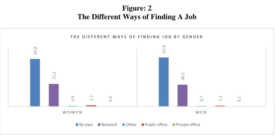
Another important issue for finding a job relies on the fact of gender differences.

Therefore, Figure 2 indicates the differences between the attitudes of women and men for

finding a job. According to the figure, both of them mostly prefer to find a job by themselves.

The percentage of this way is around 66% for women and 68% for men. Besides, the network

channels have second priority for both of them. The rate of the network is nearly the same,

around %30 for both them. The striking point of the results is that there seems to exist no

significant differences between women and men in terms of ways of finding the job.

0 10 20 30 40 50 60 70 80 2004 2005 2006 2007 2008 2009 2010 2011 2012 2013 2014 2015 2016

Figure: 2

The Different Ways of Finding A Job

The next figure, Figure 3, shows the different ways of finding jobs for different

education levels. For the higher education levels, the percentage of finding the current job

by “networks” is decreased compared to the lower levels. Besides, as education level

increases, the percentage of finding the current job by “private office” is also increasing. For

general and vocational high school graduates, percentages of finding job are similar.

Figure: 3

Different Ways of Finding the Current Job by Education

Figure 4 represents the differences between the regions (NUTS2 levels) for the

looking ways of finding the current job. It is clear that, for all different regions, the

percentage of finding the current job by “by own” is higher than the other options. The

second higher percentage is coming from finding the current job by “networks” again for all

different regions.

By own Network Other Public office Private office

2 ,3 3,9 3 4 ,5 1 9 ,8 1 0 ,8 1 1 ,8 16,9 2 ,5 3,8 3 9 ,5 1 8 ,8 11 ,7 1 3 ,1 1 0 ,7 0 ,4 ₁,4 15 ,6 1 1 ,3 1 0 ,7 ₁3,8 4 6 ,8 3, 0 5,5 3 8 ,0 2 4 ,3 1 0 ,6 1 0 ,7 7 ,9 1 ,7 ₁,3 2 0 ,6 1 2 ,0 8 ,9 11,3 4 4 ,2 I L L İ T E R A T E L İ T E R A T E P R İ M A R Y ( 5 Y R S ) S E C O N D A R Y ( 8 Y R S ) G E N E R A L H İ G H S C H O O L V O C A T İ O N A L H İ G H S C H O O L U N İ V E R S İ T Y A N D H İ G H E R D I F F E R E N T W A Y S O F F I N D I N G J O B B Y E D U C A T I O N L E V E L S

Figure: 4

Different Ways of Finding the Current Job by Regions (NUTS2)

4. Empirical Results

The tables at which the wage quantiles regression’s results are presented are given in

this section. At first, the model is estimated by employing OLS technique and then for the

quantile regression results are obtained for different quantiles (0.25, 0.50, 0.75, and 0.90

quantiles). Appendix-Table B.1 represents the OLS regression results where Table B.2

represents the quantile regressions. In Appendix Table B.2, the first column called “Total”

includes the explanatory variables such as individual characteristics, the ways of finding a

current job, years for males and females altogether. Second and third columns are females

and males, respectively. The fourth column called “Total Education” shows the model where

education dummies are included in the “Total” model. Fifth and sixth columns are the

models for females and males where the same explanatory variables are utilized in “Total

Education”. The seventh column called “Total Region” represents the model where region

dummies are included in “Total Education”. The others are again for females and males’

version of “Total Region” model

_{. Therefore, there are nine different model estimates. In the}

regressions, female, finding the current job by “own”, being inactive in the previous year,

illiterate and Istanbul denote the base category.

In this section, Table 2 is utilized in order to examine the results; however, for more

details on quantile regression results, one can look at Appendix B. In order to reveal the

changes in Table 2, the coefficients are highlighted, by doing so, a sign or significance of

the coefficients change will be seen easily. Looking at the results of the regression from

Table 2, it is examined that finding a job through social contacts leads to a decrease in wages.

6

_{Although, all the models represent in the table 2 in order to be more specific and precise only the results about}

the “Total Region” model is explained. Actually, all the coefficients in the models are significant and therefore,

there is no need to explain the other two models in the main text. The findings imply the robust results.

0 10 20 30 40 50 60 70 80 90

This result is valid not only for all different quantiles but also for all of the different models.

In addition to that, there is no significant difference with respect to gender. Although

previous studies found out that social network leads to an increase in the possibility of

finding a job, the job found by using social contacts may not be the job that the individual is

more productive. This may be because of finding a job through social contacts may lead to

a mismatch between occupational choices and productive advantages of the workers. From

this point of view, having a mismatch in the labor market results in a low return to the firm

and thus results in a decrease in aggregate productivity.

The “Total Region” model results reveal that the impact of the way of “network”

channels on wages is significant and negative for all of the different quantiles. There are

changes for “private office”, “public office” and “other” coefficients along with the different

quantiles. Although the coefficient of “private office” was positive and significant at 25

quantile regression, it loses its significance at higher quantiles. For the case of “public

office”, its effect is positive and significant at 25

_{quantile. Its effect is negative at higher}

quantiles. The impact of “other” is positive at all the quantile regression except for the

highest quantile 90

_quantiles.

Age is another controlled variable in the regression and as an individual gets older,

wage increases. Examining age variable in different quantiles of the wage distribution, it is

found out that the impact of it on the wages is valid for all the quantiles. A male dummy

variable is also added to the regressions and it is seen that being a male leads to an increase

in wages. Although the direction of the impact of being a male, the magnitude of being a

male is changing for different quantiles. For example, the lowest magnitude belongs to 0.50

quantile.

For all different quantiles, education level variables have a positive effect on wage.

In addition to that, as education level increases, the magnitude of the coefficient increases.

For the different regions, the results yield that living in Istanbul compared to living in another

region leads to decrease the wages. This is true for all different quantiles. In addition to that,

as education increases, wages increase which this is valid for all different quantiles. Previous

labor market situation of an individual has an impact on wages. As a previous year labor

market situation, being unemployed has a positive effect on wages compared to the base

category being inactive. For the case of males, being in the military, it has a positive impact

as well. However, being in the school has a negative effect on wages compared to being

inactive (Appendix B, Table B.2).

Table: 2

The Results of Quantile Regression Estimation (2004-2016)

Total Total Education Total Region

q25 Age 0.08040*** 0.06678*** 0.06317*** (0.000) (0.000) (0.000) Male 0.03794*** 0.10463*** 0.12426*** (0.000) (0.000) (0.000) Private Office 0.11012*** 0.06996*** 0.05219** (0.000) (0.000) (0.000) Public Office 0.02055*** 0.05991*** 0.12046*** (0.000) (0.000) (0.000) Network -0.07836*** -0.07842*** -0.04975*** (0.000) (0.000) (0.000) Other -0.46701*** -0.35516*** -0.32150*** (0.000) (0.000) (0.000) Constant 2.92230*** 2.83452*** 3.16616*** (0.000) (0.000) (0.000) q50 Age 0.05064*** _0.04269*** _0.04708*** (0.000) (0.000) (0.000) Male 0.02730*** _0.07701*** _0.09921*** (0.000) (0.000) (0.000) Private Office 0.10542*** _0.03496*** _-0.00153 (0.000) (0.060) (0.918) Public Office -0.04867*** _-0.02319*** _0.02348*** (0.000) (0.000) (0.000) Network -0.05410*** _-0.04727*** _-0.03201*** (0.000) (0.000) (0.000) Other -0.79792*** _-0.58427*** _-0.56107*** (0.000) (0.000) (0.000) Constant 3.79401*** _3.71376*** _3.79895*** (0.000) (0.000) (0.000) q75 Age 0.05812*** _0.03989*** _0.04085*** (0.000) (0.000) (0.000) male 0.04325*** _0.10624*** _0.11853*** (0.000) (0.000) (0.000) Private Office 0.17202*** _{0.00418 0.00364} (0.000) (0.807) (0.893) Public Office -0.14091*** _-0.08206*** _-0.05205*** (0.000) (0.000) (0.000) Network -0.07582*** _-0.04231*** _-0.03059*** (0.000) (0.000) (0.000) Other -0.02204 -0.11108*** _-0.07765** (0.000) (0.000) (0.000) Constant 3.82183*** _3.95441*** _4.07552*** (0.000) (0.000) (0.000) q90 Age 0.08135*** _0.04521*** _0.04467*** (0.000) (0.000) (0.000) male 0.03707*** _0.16453*** _0.16839*** (0.000) (0.000) (0.000) Private Office 0.17979*** _{0.02082 0.02241} (0.000) (0.511) (0.453) Public Office -0.29247*** _-0.14487*** _-0.11635*** (0.000) (0.000) (0.000) Network -0.14893*** _-0.04847*** _-0.03665*** (0.000) (0.000) (0.000) Other 0.30025*** _0.03816* _0.07979*** (0.000) (0.104) (0.000) Constant 3.66695*** _4.01241*** _4.12323*** (0.000) (0.000) (0.000) N 145138 145138 145138

Note: p values are given in parenthesis. The grey color shows the insignificant variables of the model.

*

_{p < 0.1,}

_{p < 0.05,}

_{p < 0.01.}

The obtained results of the quantile regression yield several crucial points. Firstly,

the results reveal that there exist some important differences along with the conditional

distribution of logarithmic wage distribution. At the lower tail of the wage distribution,

“private office” and “public office” coefficients are positive and significant; however, these

coefficients are negative for all other quantiles. Besides, the coefficients of “private office”

and “public office” are insignificant for the median and the 0.75 and 0.95 quantiles. This

suggests that if an individual is at the lower tail of the conditional wage distribution then the

impact of finding the job by using “private office” is positive. This is valid for the impact of

finding the job by using “public office”, as well. However, if an individual is at the upper

tail of the wage distribution then the impact of finding the job by using “private office” loses

its significance. However, the wage at the top of the distribution decreased by finding the

job by using “public office”. For the OLS results which focused on the mean effect, the

coefficients of “private office” and “public office” positive. However, the coefficient of

“private office” is insignificant. For the case of “network” and “other”, the effects are

significant and negative.

5. Conclusion

As stated from the beginning of the paper, there are many ways of searching for a

job. In Turkey, one of the most common ways of searching for a job is using informal social

networks. From this point of view, the impact of finding the way of a job can be questioned.

In this paper, the direction of the impact of informal social networks on wages is targeted.

The model is quantile regression while data is 2004-2016 HLFS. First, as an important

finding from this research is the fact that finding a job through social contact leads to a

decrease in wages. Looking at this effect on wages whether it is changing according to the

quantiles or not, the findings indicate that the result is valid for all of the quantiles. The

second one is related to gender: no significant difference between males and females via the

effects of social networks on wages. On the other hand, being a male leads to an increase in

wages for all different quantiles as expected. Examining the regional effects on wages, living

in another region other than living in İstanbul has a negative impact on wages.

Previous studies found out that social network leads to an increase in the possibility

of finding a job. However, the job found by using social contacts does not show that the

individual is more productive at that job because finding a job through social contacts may

lead to a mismatch between the workers’ occupational choices and their productive

advantages. From this point of view, having a mismatch in the labor market results in a low

return to the firm and thus results in a decrease in aggregate productivity.

Impact of finding a job through social networks on wages is found to be negative by

Mongomery (1991), Simon and Warner (1992), Casella and Hanaki (2006), Dustman et al.

(2016), Casella and Hanaki (2008), Dustmann et al. (2011), Beaman and Magruder (2012)

and Brown et al. (2012). In this study, this is valid for Turkey, as well. This negative effect

is probably due to the fact that referees do not pay attention to the ability of the applicants

during referring them for that job. Previous studies addressed the monitoring mechanism

that referees monitor the referred workers. However, as it is found out that the impact of

social networks on wages is negative, it can be said that this monitoring mechanism does

not work in Turkey. Therefore, it can be stated that social networks function as a

mismatching tool between individuals’ comparative advantage and their occupational

choices. In other words, social networks work as a proxy for unobserved characteristics for

an individual. The direction of the impact of networks on wages in Turkey looks like the one

in Greece, Italy, Portugal, and the United Kingdom.

The findings in this paper can be linked with not only the supply side but also demand

side of the labor market. It can be said that if an individual’s reservation wage is at the bottom

of the wage distribution, s/he is better off when s/he uses “private office” and “public office”

during their job search via wages. For the case of the society as a whole, using “private

office” and “public office” makes the society be better off, as well. This is because the job

at which an individual finds by using “private office” and “public office” is the one in the

occupations where the worker is more productive. For the demand side of the labor market,

hiring individuals who applied for the job by using “private office” and “public office” will

be more likely to be more efficient since in Turkey personal contacts probably leads to

mismatch. This suggestion is probably more effective for the lower tail of the wage

distribution.

References

Akerlof, G.A. & R.E. Kranton (2000), “Economics and Identity”, Quarterly Journal of Economics,

115(3), 715-53.

Akerlof, G.A. (1980), “A Theory of Social Custom, of which Unemployment may be one

Consequence”, Quarterly Journal of Economics, 94(4), 749-75.

Beaman, L.A. (2011), “Social Networks and the Dynamics of Labour Market Outcomes: Evidence

from Refugees Resettled in the U.S”, The Review of Economic Studies, 79(1), 128-161.

Beaman, L.A. & J. Magruder (2012), “Who Gets the Job Referral? Evidence from a Social Networks

Experiment”, American Economic Review, 102(7), 3574-93.

Beggs, J.J. & S.H. Jeanne (1997), “The Social Context of Men’s and Women’s Job Search Ties:

Membership in Voluntary Organizations, Social Resources, and Job Search Outcomes”,

Sociological Perspectives, 40, 601-622.

Bentolila, S. & C. Michelacci & J. Suarez (2010), “Social Contacts and Occupational Choice”,

Economica, 77, 20-45.

Bramoullé, Y. & G. Saint-Paul (2010), “Social networks and labor market transitions”, Labor

Economics, 17, 188-195.

Brass, D.J. (1985), “Men’s and Women’s Networks: A Study of Interaction Patterns and Influence in

an Organization”, Academy of Management Journal, 28, 327-43.

Brown, M. & E. Setren & G. Topa (2012), “Do informal referrals lead to better matches? Evidence

from a firm’s employee referral system”, FRB of New York Staff Report, (568).

Brown, M. & E. Setren & G. Topa (2016), “Do informal referrals lead to better matches? Evidence

from a firm’s employee referral system”, Journal of Labor Economics, 34(1), 161-209.

Buchinsky, M. (1994), “Changes in the U.S. Wage Structure 1963-1987: Application of Quantile

Regression”, Econometrica, 62(2), 405-458.

Buchinsky, M. (1998), “Recent Advances in Quantile Regression Models”, Journal of Human

Campbell, K. (1988), “Gender Differences in Job-related Networks”, Work and Occupations, 15,

179-200.

Casella, A. & N. Hanaki (2006), “Why Personal Ties cannot be Bought”, The American Economic

Review, 96(2), 261-264.

Casella, A. & N. Hanaki (2008), “Information Channels in Labor Markets: On the Resilience of

Referral Hiring”, Journal of Economic Behavior & Organization, 66(3-4), 492-513.

Drentea (1998), “Consequences of Women’s Formal and Informal Job Search Methods for

Employment in Female-Dominated Jobs”, Gender and Society, 12, 321-338.

Dustman, C. & A. Glitz & U. Schönberg & H. Brücker (2016), “Referral-based Job Search

Networks”, Review of Economic Studies, 83, 514-546.

Dustmann, C. & A. Glitz & U. Schonberg (2011), “Referral-based Job Search Networks”, IZA

Discussion Papers, 5777, Institute for the Study of Labor (IZA).

Elliot, J.R. (1999), “Social Isolation and Labor Market Insulation: Network and Neighborhood

Effects on Less-educated Urban Workers”, The Sociological Quarterly, 40, 199-216.

Franzen, A. & D. Hangartner (2006), “Social Networks and Labour Market Outcomes: The

Non-Monetary Benefits of Social Capital”, European Sociological Review, 22(4), 353-368.

Frölich, M. & B. Melly (2010), Estimation of quantile treatment effects with STATA,

<www.alexandria.unisg.ch/EXPORT/DL/60320.pdf>, 23.07.2018.

Giulietti, C. & M. Guzi & Z. Zhao & K.F. Zimmermann (2010), “Social networks and the labor

market outcomes of rural to urban migrants in China”, Working Paper, IZA.

Goel, D. & K. Lang (2009), “The Role of Social Ties in the Job Search of Recent Immigrants”,

Canadian Labour Market and Skills Researcher Network Working Paper, No. 5.

Hensvik, L. & O.N. Skans (2013), “Social networks, employee selection, and labor market

outcomes”, Institute of Evaluation of Labor Market and Education Policy Working

Paper, 2013:15.

Hölzer, H.J. (1987), “Job Search by Employed and Unemployed Youth”, Industrial and Labor

Relations Review, 40, 601-11.

Huffman, M.L. & T. Lisa (2001), “Job Search Methods: Consequences for Gender-Based Earnings

Inequality”, Journal of Vocational Behavior, 58, 127-141.

Ibarra, H. (1992), “Homophily and Differential Returns: Sex Differences in Network Structure and

Access in an Advertising Firm”, Administrative Science Quarterly, 37, 422-47.

Koenker, R. & G. Bassett (1978), “Regression Quantiles”, Econometrica, 46(1), 33-50.

Kugler, A.D. (2003), “Employee Referrals and Efficiency Wages”, Labor Economics, 10, 531-556.

Marmaros, D. & B. Sacerdote (2002), “Peer and Social Networks in Job Search”, European

Economic Review, 46, 870-79.

Mincer, J. (1974), Schooling, Experience and Earnings, Columbia University Press: New York.

Montgomery, J. (1991), “Social Networks and Labor-market Outcomes: Toward an Economic

Analysis”, The American Economic Review, 81, 1408-18.

Moore, G. (1990), “Structural Determinants of Men’s and Women’s Personal Networks”, American

Sociological Review, 55, 726-35.

Munshi, K. (2003), “Networks in the Modern Economy: Mexican Migrants in the U. S. Labor

Market”, The Quarterly Journal of Economics, 118(2), 549-599.

Pellizzari, M. (2004), “Do Friends and Relatives Really Help in Getting a Good Job?”, CEP

Discussion Paper, No 623, March.

Pistaferri, L. (1999), “Informal Networks in the Italian Labor Market”, Giornale degli Economisti e

Annali di Economia, 58, 355-75.

Saloner, G. (1985), “Old Boy Networks as Screening Mechanism”, Journal of Labor Economics, 3,

255-67.

Silliker, A.S. (1993), “The Role of Social Contacts in the Successful Job Search”, Journal of

Employment Counseling, 30, 25-34.

Simon, C. & J. Warner (1992), “Matchmaker, Matchmaker: The Effect of Old Boy Networks on Job

Match Quality, Earnings, and Tenure”, Journal of Labor Economics, 306-30.

Schmutte, I.M. (2015), “Job Referral Networks and the Determination of Earnings in Local Labor

Markets”, Journal of Labor Economics, 33(1), 1-32.

Straits, B.C. (1998), “Occupational Sex Segregation: The Role of Personal Ties”, Journal of

Vocational Behavior, 52, 191-207.

Torres, L. & M.L. Huffman (2002), “Social Networks and Job Search Outcomes among Male and

Female Professional, Technical, and Managerial Workers”, Sociological Focus, 35(1),

25-42.

APPENDIX A

Table: A.1

Ways of Finding the Current Job by Years

By own Public office Private office Network Other # of observations

2004 0.72 0.003 0.001 0.26 0.016 29072 2005 0.72 0.002 0.001 0.27 0.009 34509 2006 0.71 0.004 0.002 0.27 0.010 30505 2007 0.74 0.004 0.001 0.25 0.011 31463 2008 0.72 0.004 0.002 0.27 0.007 33971 2009 0.69 0.004 0.001 0.30 0.006 34262 2010 0.66 0.006 0.001 0.33 0.007 38559 2011 0.66 0.005 0.002 0.33 0.008 42869 2012 0.68 0.012 0.001 0.30 0.008 43306 2013 0.64 0.015 0.002 0.34 0.007 43115 2014 0.63 0.020 0.005 0.34 0.004 43953 2015 0.65 0.031 0.006 0.31 0.007 44182 2016 0.61 0.038 0.006 0.34 0.005 42985 Total 0.67 0.013 0.003 0.30 0.008 492751

Table: A.2

Ways of Finding the Current Job by Gender

By own Public office Private office Network Other # of observations

Female 0.66 0.02 0.004 0.31 0.01 130738

Male 0.68 0.01 0.002 0.30 0.01 362013

Total 0.67 0.01 0.003 0.30 0.01 492751

Table: A.3

Ways of Finding the Current Job by Education

By own Public office Private office Network Other Total

Illiterate 0.02 0.02 0.004 0.03 0.02 0.02

Literate 0.04 0.04 0.01 0.05 0.01 0.04

Primary(5 yrs) 0.34 0.40 0.16 0.38 0.21 0.35

Secondary (8 yrs) 0.20 0.19 0.11 0.24 0.12 0.21

General High school 0.11 0.12 0.11 0.11 0.09 0.11

Vocational High school 0.12 0.13 0.14 0.11 0.11 0.11

University and Higher 0.17 0.11 0.47 0.08 0.44 0.14

Table: A.4

Ways of Finding the Current Job by Regions (NUTS2)

By own Public office Private office Network Other # of observations

Istanbul (Istanbul) 0.769 0.003 0.004 0.223 0.002 75978

Tekirdag (Tekirdağ, Edirne, Kırklareli) 0.562 0.015 0.003 0.417 0.004 16697

Balikesir (Balıkesir, Çanakkale) 0.766 0.011 0.001 0.215 0.007 14374

Izmir (İzmir) 0.630 0.005 0.004 0.349 0.011 29387

Aydin (Aydın, Denizli, Muğla) 0.597 0.010 0.004 0.382 0.007 19057

Manisa (Manisa, Afyon, Kütahya, Uşak) 0.893 0.007 0.001 0.092 0.007 21665

Bursa (Bursa, Eskişehir, Bilecik) 0.710 0.008 0.003 0.277 0.002 30904

Kocaeli (Kocaeli, Sakarya, Düzce, Bolu, Yalova) 0.649 0.013 0.003 0.326 0.008 24552

Ankara (Ankara) 0.751 0.004 0.004 0.238 0.004 28840

Konya (Konya-Karaman) 0.655 0.011 0.001 0.325 0.008 25453

Antalya (Antalya, Isparta, Burdur) 0.524 0.012 0.006 0.452 0.005 18706

Adana (Adana-Mersin) 0.489 0.010 0.001 0.497 0.003 26146

Hatay (Hatay, Kahramanmaraş, Osmaniye) 0.498 0.013 0.001 0.482 0.005 16148

Kırıkkale (Kırıkkale, Aksaray, Niğde, Nevşehir, Kırşehir) 0.721 0.018 0.000 0.256 0.005 12967

Kayseri (Kayseri, Sivas, Yozgat) 0.751 0.017 0.002 0.224 0.006 10778

Zonguldak (Zonguldak,Karabük, Bartın) 0.560 0.025 0.002 0.406 0.007 7537

Kastamonu (Kastamonu, Çankırı, Sinop) 0.707 0.035 0.001 0.246 0.010 8067

Samsun (Samsun, Tokat, Çorum, Amasya) 0.547 0.017 0.002 0.419 0.016 17608

Trabzon (Trabzon, Ordu, Giresun, Rize, Artvin, Gümüşhane) 0.741 0.026 0.002 0.192 0.039 15703

Erzurum (Erzurum, Erzincan, Bayburt) 0.707 0.047 0.001 0.201 0.045 7731

Ağrı (Ağrı, Kars, Iğdır, Ardahan) 0.706 0.033 0.000 0.258 0.002 8802

Malatya (Malatya, Elazığ, Bingöl, Tunceli) 0.610 0.034 0.001 0.346 0.009 8198

Van (Vani, Muş, Bitlis, Hakkari) 0.577 0.026 0.001 0.390 0.006 10845

Gaziantep (Gaziantep, Adıyaman, Kilis) 0.629 0.014 0.001 0.351 0.005 13915

Sanliurfa (Şanlıurfa, Diyarbakır) 0.729 0.017 0.001 0.246 0.007 14456

Mardin (Mardin, Batman, Şırnak, Siirt) 0.687 0.027 0.001 0.263 0.022 8237

APPENDIX B

Table: B.1

OLS Regression Results

Total Region Female Region Male Region

Age 0.05672*** _0.03789*** _0.07318*** (65.25) (21.43) (72.85) Age2 -0.00070*** _-0.00050*** _-0.00091*** (58.59) (19.67) (66.06) Literate 0.14956*** _0.14119*** _0.11552*** (12.72) (7.12) (7.7) Primary 0.15963*** _0.13671*** _0.12793*** (15.87) (8.58) (9.55) Secondary 0.16143*** _0.15089*** _0.12209*** (15.63) (8.96) (9.00) Highschool 0.34739*** _0.42875*** _0.25648*** (32.87) (25.12) (18.43) Voc-Highschool 0.40294*** _0.49313*** _0.31285*** (37.76) (28.31) (22.38)

Uni & Higher 0.74209*** _0.83487*** _0.62933***

(70.48) (49.4) (45) Male 0.14794*** (41.52) Unemployed(t-1) 0.16936*** _0.10399*** _0.09068*** (38.07) (16.15) (11.15) Military (t-1) 0.25105*** _{NA 0.19596}*** (37.13) (.) (20.74) In school (t-1) -0.08543*** _-0.12432*** _-0.15137*** (14.98) (14.35) (16.16) Private Office 0.0283 0.05627 0.00493 (1.13) (1.4) (0.15) Public Office 0.06787*** _0.19061*** _-0.01912 (6.8) (11.77) (1.50) Network -0.06017*** _-0.08536*** _-0.04241*** (19.73) (14.68) (12.19) Other -0.23243*** _-0.23372*** _-0.23089*** (19.36) (11.29) (15.88) Year-2005 0.18572*** _0.15523*** _0.19956*** (22.98) (9.49) (22.3) Year-2006 0.41445*** _0.40207*** _0.41803*** (51.6) (25.22) (46.57) Year-2007 0.64798*** _0.62351*** _0.65963*** (81.02) (39.57) (73.49) Year-2008 0.86120*** _0.83989*** _0.87376*** (107.89) (53.3) (97.64) Year-2009 0.97215*** _0.92497*** _0.99546*** (123.61 (59.22) (113.27) Year-2010 1.14160*** _1.10712*** _1.16029*** (151.62) (72.95) (138.86) Year-2011 1.31905*** _1.26856*** _1.34670*** (177.15) (85.01) (162.53) Year-2012 1.51274*** _1.49183*** _1.53076*** (201.21) (100.16) (181.85) Year-2013 1.67197*** _1.62396*** _1.70691*** (221.06 (110.26) (199.41) Year-2014 1.87304*** _1.81390*** _1.91483*** (246.54 (122.54) (222.75) Year-2015 2.03895*** _1.98263*** _2.07723*** (269.38) (134.76) (242.1) Year-2016 2.29723*** _2.24521*** _2.32986*** (297.29) (150.62) (264.64) Tekirdag -0.27495*** _-0.26319*** _-0.28753*** (32.35) (18.54) (27.26) Balikesir -0.32555*** _-0.33867*** _-0.31567*** (38.66) (22.71) (31.57) Izmir -0.21941*** _-0.22781*** _-0.21166*** (33.62) (19.30) (27.67) Aydin -0.31410*** _-0.33031*** _-0.30170*** (38.51) (23.83) (30.23) Manisa -0.30986*** _-0.29528*** _-0.31175*** (40.99) (20.58) (36.11)

Total Region Female Region Male Region Bursa -0.22327*** _-0.26415*** _-0.19466*** (34.24) (23.12) (24.94) Kocaeli -0.20076*** _-0.24825*** _-0.17039*** (28.94) (19.54) (21.11) Ankara -0.13925*** _-0.17678*** _-0.11578*** (21.53) (15.00) (15.35) Konya -0.37177*** _-0.46574*** _-0.31922*** (51.72) (34.80) (38.51) Antalya -0.23152*** _-0.27552*** _-0.19519*** (27.51) (19.38) (18.85) Adana -0.39929*** _-0.42696*** _-0.38720*** (59.24) (33.25) (50.39) Hatay -0.38860*** _-0.46542*** _-0.35963*** (46.20) (27.56) (38.38) Kirikkale -0.27632*** _-0.29949*** _-0.26914*** (29.74) (16.39) (25.79) Kayseri -0.26080*** _-0.31534*** _-0.23444*** (26.30) (15.62) (21.36) Zonguldak -0.30752*** _-0.38547*** _-0.26538*** (26.88) (18.14) (20.10) Kastamonu -0.29512*** _-0.29240*** _-0.28358*** (26.48) (14.31) (21.88) Samsun -0.33523*** _-0.41702*** _-0.29408*** (39.70) (26.80) (30.04) Trabzon -0.22818*** _-0.26900*** _-0.21216*** (28.72) (17.64) (23.51) Erzurum -0.18942*** _-0.25973*** _-0.16513*** (17.53) (11.12) (14.11) Ağrı -0.16082*** _-0.20310*** _-0.15468*** (13.79) (7.48) (12.50) Malatya -0.26445*** _-0.27760*** _-0.25880*** (24.98) (12.73) (22.19) Van -0.12388*** _-0.17074*** _-0.12398*** (13.78) (6.26) (13.54) Gaziantep -0.30626*** _-0.38743*** _-0.28365*** (35.50) (20.54) (30.39) Sanliurfa -0.20304*** _-0.12668*** _-0.22569*** (24.24) (6.04) (25.69) Mardin -0.27350*** _-0.16193*** _-0.30094*** (26.59) (6.52) (27.82) Constant 3.42665*** _3.84441*** _3.39067*** (184.54) (112.44) (147.59) Observations 145138 49254 95884

Table: B.2

Quantile Regression Results

Total Female Male Total Education Female Education Male Education Total Region Female Region Male Region q25 Age 0.08040*** _0.08924*** _0.08762*** _0.06678*** _0.05042*** _0.07750*** _0.06317*** _0.04890*** _0.07459*** (61.03) (22.00) (66.59) (66.14) (20.52) (73.70) (56.32) (17.53) (56.79) Age2 -0.00109*** _-0.00136*** _-0.00117*** _-0.00085*** _-0.00069*** _-0.00099*** _-0.00081*** _-0.00067*** _-0.00096*** (-56.53) (-21.37) (-61.42) (-53.43) (-17.35) (-65.28) (-51.61) (-15.25) (-53.16) Male 0.03794*** _0.10463*** _0.12426*** (9.01) (19.97) (27.29) Unemployed(t-1) 0.31811*** _0.33177*** _0.06222*** _0.23335*** _0.14791*** _0.11359*** _0.18985*** _0.10408*** _0.09377*** (36.41) (29.66) (4.07) (34.90) (24.37) (10.27) (27.06) (14.54) (10.48) Military (t-1) 0.47514*** _{0.00000 0.24685}*** _0.33787*** _{0.00000 0.25226}*** _0.28210*** _{0.00000 0.21548}*** (50.17) (.) (15.79) (38.60) (.) (22.62) (32.93) (.) (21.50) In school (t-1) -0.11220*** _-0.06776*** _-0.36139*** _-0.18360*** _-0.17653*** _-0.31995*** _-0.21744*** _-0.19728*** _-0.34051*** (-9.17) (-2.86) (-20.11) (-16.75) (-17.34) (-20.97) (-19.97) (-21.09) (-32.75) Private Office 0.11012*** _0.13300*** _0.08610*** _0.06996*** _0.13757*** _{0.04012 0.05219}** _0.08380*** _0.02091 (5.82) (3.76) (3.09) (4.59) (4.38) (1.50) (2.00) (3.55) (0.75) Public Office 0.02055*** _0.09501*** _-0.00993** _0.05991*** _0.16506*** _{-0.00399 0.12046}*** _0.23728*** _0.04962*** (4.90) (6.31) (-2.40) (10.59) (9.37) (-0.67) (24.44) (16.72) (4.47) Network -0.07836*** _-0.17650*** _-0.04665*** _-0.07842*** _-0.10702*** _-0.05222*** _-0.04975*** _-0.07576*** _-0.03203*** (-15.48) (-15.94) (-14.46) (-18.31) (-12.09) (-17.54) (-11.24) (-9.86) (-6.85) Other -0.46701*** _-0.61194*** _-0.40547*** _-0.35516*** _-0.33595*** _-0.34983*** _-0.32150*** _-0.31686*** _-0.31320*** (-38.31) (-20.12) (-20.66) (-30.50) (-15.94) (-27.33) (-33.58) (-9.47) (-17.55) Year-2005 0.20016*** _0.18712*** _0.19942*** _0.19165*** _0.16046*** _0.20480*** _0.20410*** _0.17843*** _0.21955*** (20.47) (7.15) (23.43) (16.97) (4.95) (18.71) (18.88) (8.74) (37.22) Year-2006 0.42017*** _0.44801*** _0.41183*** _0.40416*** _0.42856*** _0.40033*** _0.42631*** _0.43611*** _0.42843*** (48.88) (21.89) (54.07) (31.98) (17.68) (37.94) (40.20) (18.99) (44.54) Year-2007 0.62747*** _0.66346*** _0.61865*** _0.62746*** _0.63646*** _0.61505*** _0.65674*** _0.66104*** _0.65563*** (56.62) (27.70) (86.16) (65.88) (26.64) (70.10) (67.57) (30.02) (82.53) Year-2008 0.84027*** _0.86858*** _0.83101*** _0.84138*** _0.86522*** _0.83262*** _0.87171*** _0.88960*** _0.87004*** (79.09) (44.93) (110.36) (78.79) (39.25) (99.23) (76.38) (48.94) (87.68) Year-2009 0.97637*** _0.94941*** _0.97752*** _0.96356*** _0.94668*** _0.96921*** _0.98715*** _0.98012*** _0.99950*** (92.29) (36.76) (126.43) (88.35) (42.70) (71.15) (104.84) (42.79) (117.95) Year-2010 1.15524*** _1.14600*** _1.15538*** _1.13879*** _1.12210*** _1.15089*** _1.15703*** _1.14147*** _1.17388*** (123.89) (56.66) (145.19) (96.54) (56.69) (92.50) (138.55) (48.86) (110.89) Year-2011 1.33394*** _1.31408*** _1.34152*** _1.31880*** _1.29321*** _1.33026*** _1.33847*** _1.31200*** _1.35843*** (115.62) (71.65) (208.30) (117.62) (54.04) (153.47) (137.18) (68.11) (146.47) Year-2012 1.53492*** _1.55383*** _1.52720*** _1.51852*** _1.51272*** _1.51563*** _1.53540*** _1.53312*** _1.54482*** (164.62) (82.18) (197.92) (145.63) (66.54) (160.57) (162.58) (66.19) (144.08) Year-2013 1.69924*** _1.69062*** _1.70458*** _1.67089*** _1.63092*** _1.69102*** _1.68420*** _1.65508*** _1.71164*** (149.44) (80.65) (192.31) (129.70) (66.74) (189.44) (186.76) (81.00) (158.29) Year-2014 1.90192*** _1.89403*** _1.90798*** _1.87340*** _1.81747*** _1.89794*** _1.89320*** _1.83360*** _1.92615*** (146.33) (85.20) (273.20) (216.46) (98.89) (197.39) (177.95) (87.03) (157.36) Year-2015 2.07608*** _2.07219*** _2.08356*** _2.04630*** _1.97262*** _2.07292*** _2.06088*** _2.00232*** _2.09390*** (239.58) (146.22) (214.82) (183.03) (89.30) (223.83) (209.27) (82.29) (253.48) Year-2016 2.38136*** _2.35166*** _2.38575*** _2.32292*** _2.26281*** _2.35090*** _2.33301*** _2.27732*** _2.36577*** (250.14) (150.80) (362.99) (257.28) (93.66) (220.93) (207.33) (114.54) (276.43)

Total Female Male Total Education Female Education Male Education Total Region Female Region Male Region Literate 0.17625*** _0.21687*** _0.11259*** _0.15009*** _0.16650*** _0.09985*** (7.38) (4.30) (5.67) (11.49) (4.40) (4.89) Primary 0.22141*** _0.18146*** _0.16889*** _0.18423*** _0.18047*** _0.12689*** (9.08) (4.52) (13.84) (13.90) (6.54) (6.20) Secondary 0.19240*** _0.15406*** _0.14682*** _0.15557*** _0.12170*** _0.11194*** (8.08) (3.76) (10.88) (11.10) (3.38) (5.35) Highschool 0.36996*** _0.55025*** _0.25560*** _0.33155*** _0.46867*** _0.22466*** (15.40) (14.61) (20.27) (26.20) (15.58) (9.51) Voc-Highschool 0.41163*** _0.60175*** _0.30916*** _0.37525*** _0.53285*** _0.26750*** (16.44) (14.65) (22.38) (28.41) (18.00) (13.11) Uni & Higher 0.60628*** _0.78288*** _0.45507*** _0.57490*** _0.73876*** _0.42368***

(23.59) (19.36) (32.88) (42.67) (25.12) (21.04) Tekirdag -0.24021*** _-0.25986*** _-0.23564*** (-22.03) (-17.92) (-14.06) Balikesir -0.32241*** _-0.38836*** _-0.28067*** (-33.27) (-32.73) (-28.47) Izmir -0.19556*** _-0.23521*** _-0.17449*** (-40.65) (-21.89) (-20.01) Aydin -0.30974*** _-0.37590*** _-0.25459*** (-28.79) (-16.44) (-25.23) Manisa -0.28967*** _-0.33320*** _-0.25943*** (-38.48) (-21.49) (-37.48) Bursa -0.17846*** _-0.24743*** _-0.15389*** (-26.28) (-17.96) (-23.95) Kocaeli -0.19161*** _-0.27075*** _-0.15486*** (-26.80) (-13.71) (-19.32) Ankara -0.14881*** _-0.21044*** _-0.12175*** (-19.05) (-15.74) (-16.27) Konya -0.36827*** _-0.56067*** _-0.28489*** (-37.01) (-20.35) (-29.05) Antalya -0.22106*** _-0.29377*** _-0.17756*** (-17.30) (-16.04) (-14.95) Adana -0.43910*** _-0.49568*** _-0.39008*** (-54.30) (-35.28) (-35.45) Hatay -0.41903*** _-0.55480*** _-0.35093*** (-54.88) (-21.08) (-25.56) Kirikkale -0.29897*** _-0.37764*** _-0.25542*** (-27.27) (-17.45) (-25.43) Kayseri -0.25653*** _-0.37994*** _-0.22519*** (-27.21) (-15.01) (-20.36) Zonguldak -0.32241*** _-0.43770*** _-0.25854*** (-35.06) (-15.07) (-15.44) Kastamonu -0.31813*** _-0.36903*** _-0.27048*** (-19.72) (-13.23) (-22.86) Samsun -0.38381*** _-0.48561*** _-0.32585*** (-27.96) (-24.64) (-24.77) Trabzon -0.26939*** _-0.32861*** _-0.23881*** (-41.98) (-23.19) (-24.34) Erzurum -0.21810*** _-0.33071*** _-0.18529*** (-22.59) (-13.28) (-17.29) Ağrı -0.26753*** _-0.32924*** _-0.25262*** (-21.33) (-8.79) (-22.52)