Selçuk J. Appl. Math. Selçuk Journal of Vol. 12. No. 1. pp. 43-52, 2011 Applied Mathematics
Analysis of Dominating Subset with Minimal Weight Problem Burak Ordin, Fidan Nuriyeva
Department of Mathematics, Faculty of Science, Ege University, 35100 Bornova, Izmir, Turkiye
e-mail:burak.ordin@ ege.edu.tr,nuriyevafidan@ gm ail.com
Received Date: December 11, 2009 Accepted Date: December 29, 2010
Abstract. The paper deals with the analysis of the combinatorial problem “dominating subset with minimal weight” problem that is equivalent to a sub-problem in the cutting angle method which has been developed for solving a broad class of global optimization problems. An example is given for a more clear expression of the problem and its presentation is supported by simple graph notation. Then the complexity of the problem is discussed. It is proven that the problem is strongly NP-Complete by using the weighted set covering problem. Finally analysis of dominating subset with minimal weight problem is expressed for problems in small dimensions.
Key words: Combinatorial Optimization; NP-Complete in the strong sense; Dominating Subset with Minimal Weight Problem; Weighted Set Covering Prob-lem; Set Covering Problem.
2000 Mathematics Subject Classification: 68Q25, 90C27, 65K05. 1. Introduction
The cutting angle method (CAM) for global optimization is introduced and studied in [1], [6], [8], [10]. It is an iterative method and in each iteration of CAM a subproblem has to be solved in turns, generally, a global optimization problem. Let (
) be an ∗ matrix, > , with m rows = 1, . . . , , and
columns, = 1, . . . , . All the elements of
are nonnegative. The first rows
of matrix (
) form a diagonal matrix, i.e., 0, only for = , = 1 .
Let us introduce the function : () = max
∈(min)
, where () = { : ()
The subproblem is formulated as follows: = min ∈ () subject to ∈ = {| X =1 = 1 > 0 = 1 }
The solution of the subproblem is the crucial step in CAM and reformulation of the subproblem as dominating subset with minimal weight (DSMW) problem demonstrates that the approximation is very efficient for the solution ([6-8]). In this work, DSMW problem is expressed in detail and an example is given for a more clear expression of the problem. Besides, it is presented as a mathematical model of DSMW problem and proved that this problem is NP-Complete in the strong sense. The presentation of the problem is supported by simple graph notation. Finally analysis of DSMW problem is expressed for problems in small dimensions.
The organization of the paper is as follows. In section 2, we give the definition of DSMW problem. It consists of an applied interpretation, an example and the mathematical model of the problem. In section 3 a simple graph notation has been developed for the presentation of the problem. Section 4 deals with the analysis of the problem.
2. A Brief Introduction to DSMW Problem
We will start this section with an interpretation of DSMW problem. Let () be a * matrix, with rows, = 1, 2, . . . , and columns, = 1, 2, . . . , and are non-negative for all .
The task is to choose some elements of the matrix such that:
(i) each row contains a chosen element, or contains some element which is less than some chosen element located in its column;
(ii) the sum of the chosen elements is minimal.
Let us give the following applied interpretation of this problem:
A task consisting of ( = 1, 2, . . . , ) operations can be performed by ( = 1, 2, . . . ,) processors. Suppose that the matrix () gives the time necessary for accomplishment of the task as follows: If
(1) 1 6 2 6 6
for column , then 1
is the time (or cost) required for the accomplishment of
operation 1 by processor ; 2is the time required for the accomplishment of
operations 1and 2by processor i; and so on. At last
the accomplishment of all operations ( 1 2, . . . , j ) by processor . The
problem is to distribute operations among the processors minimizing the total time (or the total cost) required for the accomplishment of all tasks. Clearly, the problem is generalized as the assignment problem ([7]).
2.1. An Example of DSMW Problem
In the following example, the DSMW problem is expressed in a simple way. Example 1. Suppose that matrix () for DSMW problem is given as in Figure 1. () = ⎛ ⎜ ⎜ ⎝ 9 4 2 3 12 8 10 1 6 5 7 11 ⎞ ⎟ ⎟ ⎠
Figure 1. DSMW problem matrix
Here, 1
1= 9 is the time (or cost) required for the accomplishment of operations
1, 2, 4 by processor 1. 2
1= 3 is the time (or cost) required for the
accomplish-ment of only operation 2 by processor 1. 3
1= 10 is the time (or cost) required
for the accomplishment of operations 1,2,3,4 by processor 1. 4
1= 5 is the time
(or cost) required for the accomplishment of operations 2 and 4 by processor 1. Likewise, 1
2 = 4 is the time (or cost) required for the accomplishment of
operations 1,3 by processor 2. 2
2 = 12 is the time (or cost) required for the
accomplishment of all operations by processor 2. 32 = 1 is the time (or cost) required for the accomplishment of just operation 3 by processor 2. 42 = 7 is the time (or cost) required for the accomplishment of operations 1, 3, 4 by processor 2. Lastly, 1
3 = 2 is the time (or cost) required for the
accomplish-ment of only operation 1by processor 3. 2
3 = 8 is the time (or cost) required
for the accomplishment of operations 1, 2, 3 by processor 3. 3
3= 6 is the time
(or cost) required for the accomplishment of operations 1, 3, 4 by processor 3. 4
3= 11 is the time (or cost) required for the accomplishment of all operations
by processor 3.
The problem is to distribute operations among the processors while minimizing the total time (or the total cost) required for the accomplishment of all tasks. A feasible solution could be given by choosing element 3
1 Then, the value
of the objective function is 10. Optimal solution of this problem is found by choosing elements 1
3 32 and 41 and the value of the objective function is that
1
2.2 Mathematical Model of the DSMW Problem
The mathematical model of the DSMW problem is constructed as follows. Let us define the function () and variables :
() = ½ 1 if ≥ 0 0 if 0 = ½ 1 if is chosen 0 otherwise
Then, the mathematical model of the DSMW problem is given as follows:
(2) min X =1 X =1 (3) X =1 6 1 = 1 2 (4) X =1 6 1 = 1 2 (5) X =1 X =1 > 1 (6) X =1 > 1 = 1 2 (7) = 0 ∨ 1 = 1 2 ; = 1 2 (8) = ( max =1{ } − ) = 1 2 ; = 1 2
Theorem 1. The Subproblem in CAM and DSMW problem are equivalent. Minimization of the subproblem in CAM is essentially a combinatorial problem, and thus grows exponentially if all possibilities are tested. DSMW problem re-duces the complexity of the crucial step in subproblem of cutting angle method. It is a new approach for solving the subproblem in the CAM by using theorem 1.
3. The Notation of DSMW Problem by Graphs
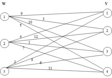
DSMW problem can be thought as a minimal matching in a bipartite graph (Figure 3.1). Suppose that, the vertices W=(w1, w2, ..., w) in the first part
of the graph G = (W, V, E) express processors and the vertices V=(v1, v2,
..., v) in the second part of G express the tasks. Each edge ∈ (the edge
=(w, v)) corresponds to the element in the matrix (
). When the value
is defined as the weight of edge , it is chosen as an acceptable matching such that its total weight is minimum and it covers all vertices of V. Among the outgoing edges of each point in W, it is called the dominant element which is greater than the others. When any dominant edge is chosen, it means that other elements which are not dominant are chosen along with the dominant element. (A dominant edge is denoted by a line and a non dominant edge is denoted by a broken line in Figure 3). But, in this case, we take only the weight of dominant edge. If some elements in set V are end points of the chosen edge then it means that those vertices are covered.
Example 2. The problem in example 1 is denoted as follow.
There is a bipartite graph that consists of two parts for the matrix () as in Figure 2, where W={1, 2, 3} and V={1, 2, 3, 4}.
1
1= 9 is the dominant of elements 21= 3 and 41= 5 in Figure 1, since 11 21
and 1
1 41. But 31 11, and so 31 = 10 is the dominant of the element
1 1= 9.
1= 31= 10 is the heaviest element of first column, so that, it covers all rows
of that column. That is, it is a dominant subset. While 3
1= 1, the others are
equal to 0, so there is an appropriate solution.
Same operations are valid for the heaviest elements of the other columns. The set {1
3= 2 32 = 1 41= 5} is a dominating subset with minimal weight
for this example. In the second row, the element 2
1 = 3 is not chosen and is
covered by 4
1= 5, because 41is the dominant of 21, so 41 is chosen.
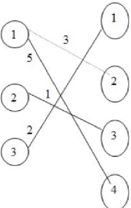
Consequently, ∗ = {1
3 = 32 = 41= 1 11 = 21 = 31= 12 = 22= 42 = 23 =
33= 43= 0} is an optimal solution and the value of the objective function is 8. Appropriate edges chosen in an optimal solution are denoted in Figure 2. These are the edges 13 = (3 1) 32 = (2 3) and 41 = (1 4). The edge 21 = (1 2) is
denoted by a broken line, because the edge 4
1= (1 4) , which is an outgoing edge
from the same vertex with 2
1, has greater weight (41 21). Only the weight of
the chosen matching is taken (2
1 = 3 is not taken) and then all vertices of set
V are covered.
4. Analysis of DSMW Problem
In this section, we prove that DSMW problem is NP-Complete in the strong sense by using weighted set covering problem. Weighted set covering problem could be defined as follow.
4.1. Weighted Set Covering Problem (WSCP)
At first, let us introduce the Set-Covering problem. An instance (X,F) of the Set-Covering problem consists of a finite set X and a family F of subsets of X such that every element of X belongs to at least one subset in F:
= [
∈
We say that a subset S∈F covers its elements. The problem is to find a maximum size subset C⊆F whose members cover all of X:
= [
∈
We say that any C satisfying above equation covers X.
It is known that this problem is NP-complete in the strong sense [8].
Theorem 2. The vertex cover problem is polynomially transformable to the set-covering problem. Therefore, the set-covering problem is NP-Complete. In [2], the WSCP is interpreted as follows: The data of the problem con-sists of finite sets 1 2 and positive numbers 1 2 . We
de-note S(: 16 6 ) by and write I={1,2,. . . ,m}, J={1,2,. . . ,n}. A
sub-set ∗ ⊆ is called a cover if S(
: ∈ ∗) = ; the cost of this cover is
P
( : ∈ ∗). The problem is to find a cover with minimum cost. This
prob-lem could be thought such that:
Let us define an mxn matrix = () where = ½
1 if ∈
0 otherwise . So, columns of A are the incidence vectors of 1 2 . Clearly, the incidence
vector = () of an arbitrary cover satisfies :
P
=1
> 1for all i,
> 0for all j.
Let be a positive row vector of length and let be the column vector whose
all m components are ones. The set covering problem is to minimize subject
to > and = 0 ∨ 1.
Let us take a WSCP instance with pxn=q variables and conditions that is equal to DSMW problem. The coefficients of the objective function in this problem are determined as follows:
1 = 11, 2 = 21,. . . , = 1, +1 =12, +2 = 22,. . . , 2 = 2, 2+1
=1
3,. . . , = .
In other words, = and t = p.(i-1) .j, 16 6 substitutions are
per-formed.
Suppose that = for some ; namely, is an element of column and
row of matrix (
) and it satisfies condition (1) for column . Besides, let
be the element of the sequence in respect of (1). Then,
1 = 2 = = = 1 and +1 = +2 = = = 0.
So, there are ones as the dominance degree of the element
= that is in
column k of matrix () (according to (1), it corresponds to first s elements) and zeros for − elements (according to (1), it corresponds to last − elements). We determine the elements of the matrix () as follows,
= ½ 1 if ≤ 0 if
and the problem is formulated as,
(9) min X =1 (10) X =1 > 1 = 1 2 (11) = 0 ∨ 1 = 1 .
The problem (9)-(11) is a WSCP where each column of the matrix () corre-sponds to some in [2]. Here t=p*(i-1)+j.
It is clear that, all operations in this transformation are bounded by (3).
Since we determine the number = ∗ for elements = , and the number
∗ = 2∗ for elements
, so, () operation is performed.
4.2. Some Properties of DSMW Problem
Let us take a decision version of DSMW problem, D(DSMW). Each I∈D(DSMW) instance is determined by a given matrix () and a real number . The aim is to find if there exist such that the value of the objective function does not exceed ? The following functions could be used as Length and Max functions for D(DSMW) problem.
Length[I]=¯¯¯()¯¯¯ = ∗
[] = max{| = 1 ; = 1 }
Now, let us give some Lemmas about D(DSMW). Lemma 1. D(DSMW) problem is a number problem.
Proof:In DSMW problem, there aren’t any bounds for numbers . Therefore, there is no polynomial , such that []6 ([]), ∀I∈D(DSMW). Then, D(DSMW) is a number problem.
Lemma 2. D(DSMW)∈ NP
Proof: It is clear that, the answer in any solution is either yes or no and for checking this answer, () operation is performed. A chosen cover set consists of at most elements, furthermore the number of the operations done for checking whether it covers the matrix or not, is bounded by () To compute its weight and compare with , () operation is required. Consequently, the number of the total operation is bounded by () Namely, D(DSMW) ∈ NP.
Theorem 3. D(DSMW) problem is NP-Complete in the strong sense.
Proof: As seen in section 4.1, WSCP is polynomially transformable to DSMW problem. Besides, Set Covering Problem (SCP), which is a special type of WSCP where 1 2 = 1, is NP-Complete and it is not a number problem.
So, SCP is NP-Complete in the strong sense ([4], [9]). For any Π ∈ D(DSMW) problem and any polynomial P, let Π denote the subproblem of Π obtained by
Π = { ∈ Π |[] 6 ([]) }, then Π is not a number problem. So,
according to Lemma 1 and Lemma 2, D(DSMW) problem is NP-Complete in the strong sense.
Analysis of DSMW problem in small dimensions could be given as follows. DSMW problem (where ∗ is the optimal solution, = 1 2 and = 1 2) is solved in polynomial time of its dimensions.
For = 1, ∗= min =1{
1
},clearly, () operation is performed.
For = 2, ∗= min{ min =1{ 1 2} ( min =1{ 1 } + min =1{ 2 })}
It is obvious that the number of the operations should be O(2n)+O(n)+O(n)=O(n). For = 1, ∗= max
=1{
1} , the number of the operations are () For = 2,
∗= min{min{max =1{ 1 } max =1{ 2} min{ min =1{ 1+ max{ 2| ∈ − ( 1)}} min =1{ 2+ max{ 1| ∈ − (2)}}}}
Here, 2() operation is performed to determine min ½ max =1 1 ¾ max =1{ 2}},
(2) operation is performed for determining min =1{ 1+max{ 2| ∈ − ( 1)}} and min =1{ 2+ max{ 1 | ∈ − ( 2)}}.
Consequently, the number of the total operations are 2.O(p)+2O(p2) = (2)
for = 2. 5. Conclusion
In this paper, the analysis of a combinatorial problem that is equal to a sub-problem in the cutting angle method which has been developed for solving a broad class of global optimization problems is expressed. The presentation of the problem is supported by simple graph notation. It is proved that the prob-lem is NP-Complete in the strong sense by using weighted set covering probprob-lem. For small values (n=1, 2 and p=1, 2), the problem could be solved in polynomial time analytically.
References
1. Dj. Babayev, A.(2000): An Exact Method for Solving the Subproblem of the Cutting Angle Method of Global Optimization In book "Optimization and Related Topics", in Kluwer Academic Publishers, series "Applied Optimization", Vol 47, De-cember, Dordrecht/Boston/ London, 472pp.
2. Chvatal, V.(1979): A Greedy Heuristic for the Set Covering Problem, Mathematics of Operations Research, 4(3):233-235.
3. Garey, R.M. and Johnson, D.S.(1979): Computers and Intractability. A Guide to the Theory of NP-Completeness., San Francisco, Freeman.
4. Johnson, D.S.(1974): Approximation Algorithms for Combinatorial Problems, Jour-nal of Computer and System Sciences, 9:256-278.
5. Lovasz, L.(1975): On the ratio of optimal integral and fractional covers, Discrete Mathematics, Vol. 13, pp. 383-390.
6. Nuriyev, U.G.(2005): An Approach to the Subproblem of the Cutting Angle Method of Global Optimization, Journal of Global Optimization, 31, 353-370.
7. Nuriyev, U.G., Ordin B.(2004): Computing Near-Optimal Solutions For The Dom-inating Subset with Minimal Weight Problem, International Journal Of Computer Mathematics, Vol 81, No 11, 1309-1318.
8. Ordin, B.(2009): “The Modified Cutting Angle Method for global minimization of increasing positively homogenius functions over the unit simplex”, Journal of Industrial and Management Optimization (JIMO), Vol 5 (4), 825-834.
9. Papadimitriou, C.H., Steiglitz, K.(1982): Combinatorial Optimization:Algorithms and Complexity, Prentice-Hall.
10. Rubinov, A.M.(2000): Abstract Convexity and Global Optimization, Kluwer Aca-demic Pub, Dordrecht.