GENERALIZED ASYMMETRIC POWER
ARCH MODELING OF NATIONAL STOCK
MARKET RETURNS
Mert URAL∗
Özet
Uygulamalı çalışmalar finansal varlık getirilerinin şişman kuyruk (leptokurtosis) özelliği sergilediklerini ve genellikle oynaklık kümelenmesi ve asimetrik yapı ile nitelendirildiklerini göstermiştir. Bu çalışmada, sekiz ülkenin ulusal borsa endeks getirilerinde (Nasdaq100, DAX, Nikkei225, Strait Times, MerVal, IPC, Shanghai Composite and ISE100) farklı hata dağılımlarına bağlı olarak oynaklık yapılarını belirlemek üzere Ding, Granger and Engle (1993) tarafından ileri sürülen Genelleştirilmiş Asimetrik Üslü ARCH (APGARCH) modelinin uygulanabilirliği araştırılmıştır. Çalışmanın bulguları, piyasalarda yaşanan gelişmelere karşı asimetrik etkilerin varlığında, finansal zaman serilerindeki çarpıklık ve basıklık özelliklerini birlikte ele alan çarpık Student-t dağılımlı APGARCH(1,1) modelinin tercih edilmesi gerektiği yönündedir.
Anahtar Kelimeler: APGARCH, çarpık Student-t dağılımı, borsa endeks getirileri JEL Sınıflandırması: C22, C52, G12, G15
Abstract
Empirical studies have shown that a large number of financial asset returns exhibit fat tails (leptokurtosis) and are often characterized by volatility clustering and asymmetry. This paper considers the ability of the Generalized Asymmetric Power ARCH (APGARCH) model introduced by Ding, Granger and Engle (1993) to capture the stylized features of volatility in national stock market returns for eight countries (Nasdaq100, DAX, Nikkei225, Strait Times, MerVal, IPC, Shanghai Composite ve ISE100). The results of this paper suggest that in the presence of asymmetric responses to innovations in the market, the APGARCH(1,1) Skewed Student-t model which accommodates both the skewness and the kurtosis of financial time series is preferred.
Keywords: APGARCH, skewed Student-t distribution, stock market returns JEL Code: C22, C52, G12, G15
∗ Department of Economics, Faculty of Economics and Administrative Sciences, Dokuz Eylul
INTRODUCTION
Asset returns are approximately uncorrelated but not independent through time as large (small) price changes tend to follow large (small) price changes. This temporal concentration of volatility is commonly referred to as volatility clustering and it was not fully exploited for modeling purposes until the introduction of the ARCH model by Engle (1982) and Generalized ARCH (GARCH) model by Bollerslev (1986). There have been numerous developments in the ARCH literature to refine both the mean and variance equations, in order to better capture the stylized features of high frequency data. A common feature of the standard class of ARCH models is that they relate the conditional variance to lagged squared residuals and past vari-ances.
The ARCH literature has developed so rapidly. One recent develop-ment in the ARCH literature has focused on the power term by which the data is to be transformed. Ding, Granger and Engle (1993) introduced a new class of ARCH model called the Power ARCH model which estimates the optimal power term. They also found that the absolute returns and their pow-er transformations have a highly significant long-tpow-erm memory proppow-erty as the returns are highly correlated.
Another important innovation has been development of ARCH model specifications to describe the asymmetry present in financial data. Stock market returns data commonly exhibits an asymmetry in that positive and negative shocks to the market do not bring forth equal responses. This phe-nomenon most commonly attributed to the leverage effect (see Black 1976, Christie 1982 and Nelson 1991). The applicability of the Power ARCH class of model to stock market data has been well documented in papers such as Ding, Granger and Engle (1993), Hentschel (1995), Giot and Laurent (2003) and, Pan and Zhang (2006).
Because of the empirical studies have shown that a large number of fi-nancial asset returns exhibit fat tails (leptokurtosis) and asymmetry in volatility, the main purpose of this paper is to examine the adequacy of the APGARCH model to capture the stylized features of volatility in national stock market returns for eight countries. The results of this paper suggest that in the presence of asymmetric responses to innovations in the market, the APGARCH(1,1) Skewed Student-t model is preferred. However, as internal dynamics of each market are different, there is inability to judge the parameters of the model by distinguishing markets as developed and emerging markets.
The remainder of this paper proceeds as follows. In section 2 details the general model and discusses how various ARCH models are nested with-in this APGARCH structure. Section 3 describes the national stock market returns data to be used in this study and presents the empirical results. The robustness of these findings is assessed using the Akaike Information Crite-rion (AIC) and log-likelihood (LL) values. Section 4 contains some conclud-ing remarks.
METHODOLOGY
The Generalized Asymmetric Power ARCH (APGARCH) model, which was introduced by Ding, Granger and Engle (1993), is presented in the following framework:
0 t t y = + (1) c ε t zt t ε = σ (2) . . . (0,1) i i d t z f (3) 0 1 1 ( ) p q t i t i i t i j t j i j δ δ δ σ ω α ε − γ ε− β σ − = = = +
∑
− +∑
(4)where c is a constant parameter, 0 εt is the innovation process, σt is the conditional standard deviation, z is an independently and identically t distributed (i.i.d.) process. (.)f is the probability density function (PDF) and (.)F is the cumulative density function (CDF) with
0 0, i 0, j 0, 0
ω > α ≥ β ≥ δ ≥ and γi ≤ . Here 1 αi and βj are the standard ARCH and GARCH parameters, γi is the leverage parameter and δis the parameter for the power term. A positive (resp. negative) value of the γi means that past negative (resp. positive) shocks have a deeper impact on current conditional volatility than past positive (resp. negative) shocks.
The model imposes a Box and Cox (1964) transformation in the condi-tional standard deviation process and the asymmetric absolute innovations. In the APGARCH model, good news (εt i− > ) and bad news (0 εt i− < ) have 0 different predictability for future volatility, because the conditional variance depends not only on the magnitude but also on the sign ofεt.
To put Equation (4) into operation we need to specify the lag structure and in this paper a first order lag structure is adopted for both the ARCH and GARCH terms:
(
)
1 1 1 1 1 t t t t δ δ δ σ = +ω α ε− −γε− +β σ − (5) where ω α γ β, , ,1 i 1andδ are additional parameters to be estimated. Equation (5) shall hereafter be referred to as a Generalized Asymmetric Power ARCH (APGARCH) model to reflect the inclusion of the β term. Thus, we are able to distinguish this model from a version in whichβ1= , 0 that we shall refer to as an Asymmetric Power ARCH (APARCH) model.In the influential paper of Engle (1982), the density function of zt, (.)
f was the standard normal distribution. Bollerslev (1987) tried to capture the high degree of leptokurtosis that is presented in high frequency data and proposed the Student-t distribution in order to produce an unconditional distribution with fat tails. Lambert and Laurent (2001) suggested that not only the conditional distribution of innovations may be leptokurtic, but also asymmetric and proposed the Skewed Student-t densities function.
According to Lambert and Laurent (2001) and provided that υ> , the 2 innovation process z is said to be (standardized) Skewed Student-t (in short t SKST) distributed, i.e. zt SKST(0,1, , )ξ υ , if:
(
)
(
)
(
)
2 if 1 , 2 / if 1 t t t t t m sg sz m z s f z m sg sz m z s ξ υ ξ ξ ξ υ ξ υ ξ ξ ⎧ ⎡ + ⎤ < − ⎪ ⎣ ⎦ + ⎪ ⎪ = ⎨ ⎪ ⎡ + ⎤ ≥ − ⎣ ⎦ ⎪ + ⎪ ⎩ (6)where g
( )
.υ is a symmetric (unit variance) Student-t density and ξ is the asymmetric term. In short, ξ models the asymmetry, while υ accounts for the tail thickness. Parameters m and s are, respectively the mean and 2 the variance of the non-standardized Skewed Student-t density:1 2 1 2 2 m υ υ ξ υ ξ π − ⎛ ⎞ Γ⎜ ⎟ − ⎛ ⎞ ⎝ ⎠ = ⎜ − ⎟ ⎛ ⎞ ⎝ ⎠ Γ⎜ ⎟ ⎝ ⎠ (7) and 2 2 2 2 1 1 s ξ m ξ ⎛ ⎞ =⎜ + − −⎟ ⎝ ⎠ (8)
Following Ding, Granger and Engle (1993), if it exists, a stationary so-lution of Equation (5) is given by:
0 1 1 ( ) 1 ( ) t E E z z δ δ ω σ α γ β = − − − (9)
which depends on the density of z . Such a solution exist if
1 ( ) 1 1
V =α E z −γz δ +β < . The V coefficient may be viewed as a measure of volatility persistence.
Ding, Granger and Engle (1993) derived the expression for (E z −γz)δ for the Gaussian case. We can also show that for the standardized Skewed Student-t distribution is given as follows:
( ) ( )
{
}
( ) ( ) 1 2 (1 ) (1 ) 1 2 2 2 ( ) 1 1 1 2 2 E z z δ δ δ δ δ δ δ υ δ υ γ ξ γ ξ γ υ ξ υ π ξ + − + + + − ⎛ ⎞ ⎛ ⎞ Γ⎜ ⎟ ⎜Γ ⎟ − ⎝ ⎠ ⎝ ⎠ − = + + − ⎛ + ⎞ − Γ⎜ ⎟⎛ ⎞ ⎜ ⎟ ⎝ ⎠ ⎝ ⎠ (10)It is possible to nest a number of the more standard ARCH and GARCH formulations within this Asymmetric Power GARCH model by specifying permissible values for , , andα β γ δ in Equation 4. Table 1 sum-marizes the restrictions required to produce each of the models nested within this APGARCH model. From Table 1, where αiis free, δ =2 and both βj and
γ
i= 0, this model reduces to Engle’s (1982) ARCH model. Further, when we extend this model to allow both αi and βj to take on any value, we get Bollerslev’s (1986) GARCH model. The GJR-ARCH model of Glosten, Jagannathan and Runkle (1993) is obtained whereδ=2 and .βj= . 0 The Threshold ARCH (TARCH) model of Zakoian (1994) is defined wherei
model (NARCH) of Higgins and Bera (1992) is obtained where δand αi are free, and both βi and γiare 0. If we extend this NARCH model to allow
i
β to also being free, then a Power GARCH (PGARCH) specification is the result.
Insert Table 1 about here
The models nested so far have assumed a symmetrical response of vola-tility to innovations in the market. However, empirical evidence suggests that positive and negative returns to the market of equal magnitude will not generate the same response in volatility. Glosten, Jagannathan and Runkle (1993) provided one of the first attempts to model asymmetric or leverage effects with a model which utilizes a GARCH type conditional variance specification. In this GJR-GARCH model, δ=2 and βj is free however,
i
α is specified as αi
(
1+γi)
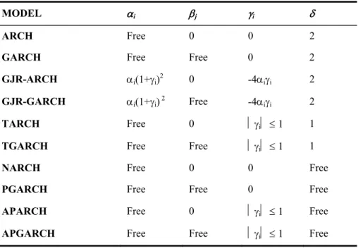
2 and leverage term is restricted to 4− α γi i. The Generalized TARCH (TGARCH) model is derived by allowing βj being free. Lastly, if αi, βj and δ are free, and γi ≤ , then an Asymmetric 1 Power GARCH specification is the result. Full details and proofs of this nesting process may be found in Ding, Granger and Engle (1993).DATA AND EMPIRICAL RESULTS
The section shows the empirical results of models. The closing prices of eight stock market price indices are analyzed. Computations were per-formed with G@RCH 4.2 which is Ox package designed for the estimation of various time series models. The characteristics of the data are presented in the first subsection. The second subsection shows the estimated results of APGARCH (1,1) Skewed Student-t model specifications and the corre-sponding qualification tests. To conserve space the GARCH (1,1) and GJR-GARCH (1,1) model results declined to present although they are available upon request. The APGARCH (1,1) model produced highly significant test statistics than GARCH (1,1) and GJR-GARCH (1,1) models. The
APGARCH model contained either a significant asymmetry term or a power term which was significantly different from two.
Data
The paper considers the national stock market closing prices for eight countries. These countries and their respective price indices are: USA (Nasdaq100), Germany (DAX), Japan (Nikkei225), Singapore (Strait Times), Argentina (MerVal), Mexico (IPC), China (Shanghai Composite) and Turkey (ISE100). The reason why these countries have been chosen is to reveal the disparity of results of the analysis and the applicability of the APGARCH (1,1) model in terms of developed (USA, Germany, Japan, Singa-pore) and emerging markets (Argentina, Mexico, China, Turkey). Country memberships for the Morgan Stanley Capital International (MSCI) Interna-tional Equity Indices have taken into consideration for market distinction. The data obtained from the Yahoo Finance: World Indices database and the Istanbul Stock Exchange for the period 04.01.1999 to 02.07.2009. For each national stock market price indices, the continuously compounded rate of return was estimated as rt =ln(pt/ pt−1) where pt is the closing price on day
t.
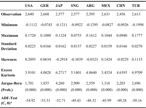
The usual descriptive statistics for each stock market return series are summarized in Table 2. It is not surprising that these series exhibit asymmet-ric and leptokurtic (fat tails) properties. Thus, the return series of these stock indices are not gauss distributed. Also the Jarque-Bera statistic is highly significant for each of the models indicating non-normality of the data. The JAP, SNG, ARG and CHN stock market returns are negatively skewed while the others positively.
Insert Table 2 about here
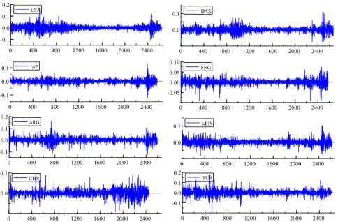
From the descriptive graphics presented in Figure 1, several volatility periods can be observed. These graphical expositions show that all of the return series exhibit volatility clustering which means that there are periods of large absolute changes tend to cluster together followed by periods of relatively small absolute changes.
Insert Figure 1 about here
Estimation Results
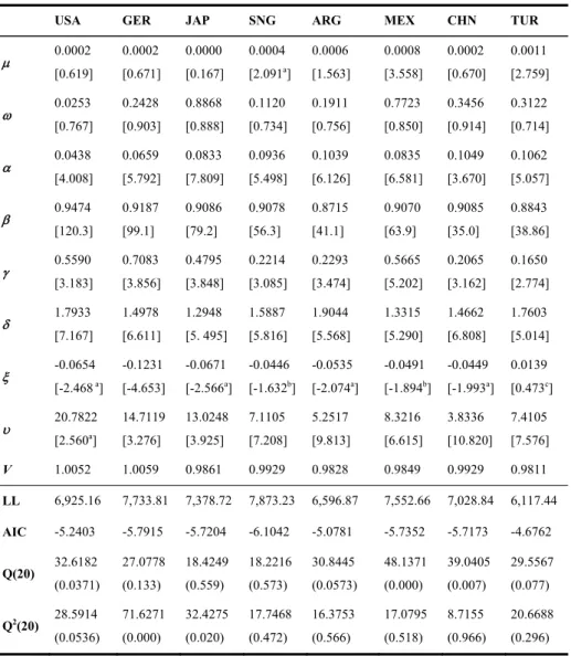
In this subsection, the APGARCH (1,1) model is estimated for each na-tional stock market return series under Gauss, Student-t, GED (Generalized Error Distribution) and Skewed Student-t distributions. The standard of model selection is based on in-sample diagnosis including Akaike Infor-mation Criterion (AIC), log-likelihood (LL) values, and Ljung-Box Q and Q2 statistics on standardized and squared standardized residuals respectively.
Under every distribution, the model which has the lowest AIC or highest LL values and passes the Q-test simultaneously is adopted. In summary, ranking by AIC and LL favours the APGARCH (1,1) Skewed Student-t specification in all national stock market return series.
Table 3 presents the results of this estimation procedure and from this table one can see that all of the ARCH and GARCH coefficients are statisti-cally significant at the 1% level. Further, the sum of the ARCH and GARCH coefficients for all of the models estimated was less than unity indicating that shocks to the model are transitory rather than permanent. Also,
β
1 is close to 1 but significantly different from 1 for all series, which indicates a high degree of volatility persistence.β
1 takes values between 0.87 to 0.95 suggesting that there are substantial memory effects. Furthermore, in USA and GER cases the APGARCH models are persistent in the sense that V coefficient is equal to 1, and in all other cases the APGARCH models are stationary in the sense that V coefficient is lower than 1.The APGARCH model includes a leverage term (
γ
) which allows pos-itive and negative shocks of equal magnitude to elicit an unequal response from the market. Table 3 presents details of this leverage term and reveals that for all models fitted; the estimated coefficient was positive and statisti-cally significant. This means that negative shocks lead to higher subsequent volatility than positive shocks (asymmetry in the conditional variance). Such a result was expected since response asymmetry is generally attributed solely to stock market data.From Table 3, the evidence of long memory process could be also found in the results of the model estimation because the power term (
δ
) of APGARCH models range in value from 1.9044 in the case of ARG to 1.2948 in the case of JAP. The average power term across all of the models estimated was 1.5796. For two of the models (MEX and JAP) estimated the power term was significantly different from two and for an additional four models (USA, SNG, ARG and TUR) estimated the power term was signifi-cantly different from unity. This means that for six of the eight models esti-mated, the optimal power term was some value other than unity or two which would seem to support the use of a model which allows the power term to be estimated. The APGARCH models the conditional standard de-viation for the MEX and JAP return series and the conditional variance for the USA, SNG, ARG and TUR return series.For the Skewed Student-t distribution, the asymmetric terms are nega-tive (ξ<0) and statistically significant for all the national stock market return series except TUR. Note that G@RCH does not estimate
ξ
but log(ξ
) to facilitate inference about the null hypothesis of symmetry (since the Skewed Student-t equals the symmetric Student-t distribution when ξ=1 or log(ξ)=0). The sign of log (ξ) indicates the direction of the skewness. The third moment is positive, and the density is skew to the right, if log (ξ)>0. On the contrary, the third moment is negative, and the density is skew to the left, if log (ξ)<0. We can confirm that the density distributions of all series are skewed to the left side due to these significantly negative asymmetric terms.The tail term (υ) is much larger for the USA, GER and JAP returns than for the other series. This means that daily returns of the SNG, ARG, MEX, CHN and TUR stock market price indices display a much larger kur-tosis and exhibit fatter tails than returns for the USA, GER and JAP stock market price indices. Besides, the evidences show that fat-tail phenomenon is strong because the student or tail terms (υ) are significantly different from zero for all series under Skewed Student-t distribution.
The results given in Table 3 show that the APGARCH succeeds in tak-ing into account all the dynamical structure exhibited by the returns and volatility of the returns as the Ljung-Box statistics for up to 20 lags on the standardized residuals (Q) non-significant at the 5% level (except USA, MEX and CHN return series) and the squared standardized residuals (Q2)
non-significant at the 5% level (except GER and JAP return series).
CONCLUSION
A recent development in the ARCH literature has been the introduction of the Power ARCH class of models which allow a free power term rather than assuming an absolute or squared term in their specification. According-ly, the purpose of the current paper was to consider the applicability of the Generalized Asymmetric Power ARCH (APGARCH) model to the selected national stock market returns for eight countries. The stock market indices were investigated by using the APGARCH (1,1) model with Skewed Stu-dent-t distribution. To capture the long memory property exhibited in the conditional variance, the power term (
δ
) estimates of APGARCH model is in the interval between one and two. It indicates that the return series of all the national stock market price indices are skewed distributed and have fat tails by the significant coefficients ofξ
(not significant for TUR) and υ in the results of model estimation. The skewed Student-t density appears to be a promising specification to accommodate both the high kurtosis and the skewness inherent to most asset returns.The estimation results indicate that strong leverage effects are present in national stock market data especially for USA, GER, JAP and MEX. Fur-ther, once these leverage effect are modeled in a GARCH framework, the inclusion of a power term is a worthwhile addition to the specification of the model. Also, in developed markets the volatility persistence is higher than emerging markets. Thus, shocks in the return series have substantial memory effects.
Consequently, in this paper, the ability of the APGARCH model is ana-lyzed so as to present the volatility characteristics of four developed and four emerging markets. The results suggest that in the presence of asymmetric responses to innovations in the market, the APGARCH(1,1) Skewed Stu-dent-t model which accommodates both the skewness and the kurtosis of
financial time series is favored. However, as internal dynamics of each mar-ket are different, it is concluded that there is no possibility to judge and to interpret the parameters of the model by differentiating markets as developed and emerging markets.
REFERENCES
Ané, T. (2006). An analysis of the flexibility of asymmetric power GARCH models,
Compu-tational Statistics and Data Analysis, 51, 1293-311.
Angelidis, T. & Degiannakis, S. (2008). Forecasting one-day-ahead VaR and intra-day realized volatility in the Athens Stock Exchange Market, Managerial Finance, 34, 489-97. Bera, A.K. & Higgins, M.L. (1993). ARCH models: properties, estimation and testing,
Jour-nal of Economic Surveys, 4, 305-62.
Black, F. (1976) Studies in stock price volatility changes, Proceedings of the 1976 Meeting of the Business and Economics Statistics Section, 177–81.
Bollerslev, T. (1986). Generalized autoregressive conditional heteroskedasticity, Journal of
Econometrics, 31, 307-27.
Bollerslev, T. (1987). A conditionally heteroskedastic time series model for speculative prices and rates of return, Review of Economics and Statistics, 69, 542-47.
Bollerslev, T., Engle, R.F. & Nelson, D.B. (1994). ARCH models, in Handbook of
Economet-rics (Ed.) Robert F. Engle and Daniel L. McFadden, North Holland Press,
Amster-dam, pp.2959–3038.
Brooks, R.D., Faff, R.W., McKenzie, M.D. & Mitchell, H. (2000). A multi-country study of power ARCH models and national stock market returns, Journal of International
Money and Finance, 19, 377–97.
Christie, A.A. (1982). The stochastic behaviour of common stock variances: value, leverage and interest rate effects, Journal of Financial Economics, 10, 407–32.
Diamandis, P.F., Kouretas, G.P. & Zarangas, L. (2006). Value-at-Risk for long and short trading positions: the case of the Athens Stock Exchange, Working Paper No:601, University of Crete, Department of Economics.
Ding, Z., Granger, W.J. & Engle, R.F. (1993). A long memory property of stock market re-turns and a new model, Journal of Empirical Finance, 1, 83-106.
Fernandez, C. & Steel, M.F.J. (1998). On bayesian modelling of fat tails and skewness,
Jour-nal of the American Statistical Association, 93, 359-71.
Giot, P. & Laurent, S. (2004). Modelling daily Value-at-Risk using realized volatility and ARCH type models, Journal of Empirical Finance, 11, 379-98.
Glosten, G.L., Jagannathan, R. & Runkle, D.E. (1993). On the relation between the expected value and the volatility of the nominal excess return on stocks, Journal of Finance, 48, 1779-801.
Härdle, W.K. & Mungo, J. (2008). Value-at-Risk and expected shortfall when there is long range dependence, SFB 649 ‘Economic Risk’ Discussion Paper No:006, 1-39. Hentschel, L. (1995). All in the family: nesting symmetric and asymmetric GARCH models,
Journal of Financial Economics, 39, 71-104.
Jondeau, E., Poon, S. & Rockinger, M. (2007). Financial Modeling Under Non-Gaussian
Distributions, Springer Finance, USA.
Jorion, P. (2007). Financial Risk Manager Handbook, 4th Edition. John Wiley&Sons Inc., USA. Lambert, P. & Laurent, S. (2001). Modelling financial time series using GARCH-type models
with a skewed student distribution for the innovations, Discussion Paper 0125, Uni-versité Catholique de Louvain, Belgium.
Laurent, S. (2004). Analytical derivates of the APARCH model, Computational Economics, 24, 51-7.
Laurent, S. (2008). G@RCH 5.0 Help, Download Date: 30.03.2009, WWW:Web: http://www. garch.org
McKenzie, M.D. & Mitchell, H. (2002). Generalized asymmetric power ARCH modeling of exchange rate volatility, Applied Financial Economics, 12, 555-64.
Pan, H. & Zhang, Z. (2006). Forecasting financial volatility: evidence from Chinese Stock Market, Working Paper in Economics and Finance No:06/02, University of Durham. Tang, T. & Shieh, S. (2006). Long memory in stock index futures markets: a Value-at-Risk
approach, Physica A, 366, 437-48.
Tsay, R.S. (2005). Analysis of Financial Time Series, 2nd Edition, John Wiley&Sons Inc., USA. Zakoian, J.M. (1994). Threshold heteroskedastic models, Journal of Economic Dynamics and
Table 1. Taxonomy of ARCH/GARCH model specifications
MODEL αi βj γi δ
ARCH Free 0 0 2
GARCH Free Free 0 2
GJR-ARCH αi(1+γi)2 0 -4αiγi 2 GJR-GARCH αi(1+γi) 2 Free -4αiγi 2
TARCH Free 0 ⏐γi⏐ ≤ 1 1
TGARCH Free Free ⏐γi⏐ ≤ 1 1
NARCH Free 0 0 Free
PGARCH Free Free 0 Free
APARCH Free 0 ⏐γi⏐ ≤ 1 Free
Table 2. Descriptive statistics
USA GER JAP SNG ARG MEX CHN TUR
Observation 2,640 2,668 2,577 2,577 2,595 2,631 2,456 2,613 Minimum -0.1112 -0.0743 -0.1211 -0.0922 -0.1295 -0.0827 -0.0926 -0.1998 Maximum 0.1720 0.1080 0.1324 0.0753 0.1612 0.1044 0.0940 0.1777 Standard Deviation 0.0225 0.0166 0.0162 0.0137 0.0227 0.0159 0.0166 0.0270 Skewness 0.2095 0.0634 -0.2918 -0.3839 -0.0323 0.1424 -0.0229 0.1115 Excess Kurtosis 3.9101 4.0828 6.2717 5.1401 4.8640 3.4524 4.6393 4.9709 Jarque-Bera (Prob.) 1,701 (0.000) 1,855 (0.000) 4,260 (0.000) 2,900 (0.000) 2,559 (0.000) 1,316 (0.000) 2,203 (0.000) 2,696 (0.000) ADF-Test (C, 0)* -54.92 -53.31 -52.71 -49.43 -48.32 -45.99 -49.28 -50.16 Note: USA: Nasdaq100 (USA), GER: DAX (Germany), JAP: Nikkei225 (Japan), SNG:
Strait Times (Singapore), ARG: MerVal (Argentina), MEX: IPC (Mexico), CHN: Shanghai Composite (China), TUR: ISE100 (Turkey).
* (C, 0) indicates that there is a constant but no trend in the regression model with lag=0. All Augmented Dickey Fuller (ADF) test statistics reject the hypothesis of a Unit Root at the 1% level of confidence. MacKinnon critical value at the 1% confidence level is -3.44.
0 400 800 1200 1600 2000 2400 -0.1 0.0 0.1 0.2 ARG 0 400 800 1200 1600 2000 2400 0.0 0.1 MEX 0 400 800 1200 1600 2000 2400 0.0 0.1 DAX 0 400 800 1200 1600 2000 2400 -0.1 0.0 0.1 JAP 0 400 800 1200 1600 2000 2400 -0.05 0.00 0.05 0.10 SNG 0 400 800 1200 1600 2000 2400 0.0 0.1 CHN 0 400 800 1200 1600 2000 2400 -0.1 0.0 0.1 0.2 USA 0 400 800 1200 1600 2000 2400 -0.1 0.0 0.1 0.2 TUR
Note: USA: Nasdaq100 (USA), GER: DAX (Germany), JAP: Nikkei225 (Japan), SNG:
Strait Times (Singapore), ARG: MerVal (Argentina), MEX: IPC (Mexico), CHN: Shanghai Composite (China), TUR: ISE100 (Turkey).
Table 3. APGARCH (1,1) skewed Student-t model estimation results
USA GER JAP SNG ARG MEX CHN TUR
μ 0.0002 [0.619] 0.0002 [0.671] 0.0000 [0.167] 0.0004 [2.091a] 0.0006 [1.563] 0.0008 [3.558] 0.0002 [0.670] 0.0011 [2.759] ω 0.0253 [0.767] 0.2428 [0.903] 0.8868 [0.888] 0.1120 [0.734] 0.1911 [0.756] 0.7723 [0.850] 0.3456 [0.914] 0.3122 [0.714] α 0.0438 [4.008] 0.0659 [5.792] 0.0833 [7.809] 0.0936 [5.498] 0.1039 [6.126] 0.0835 [6.581] 0.1049 [3.670] 0.1062 [5.057] β 0.9474 [120.3] 0.9187 [99.1] 0.9086 [79.2] 0.9078 [56.3] 0.8715 [41.1] 0.9070 [63.9] 0.9085 [35.0] 0.8843 [38.86] γ 0.5590 [3.183] 0.7083 [3.856] 0.4795 [3.848] 0.2214 [3.085] 0.2293 [3.474] 0.5665 [5.202] 0.2065 [3.162] 0.1650 [2.774] δ 1.7933 [7.167] 1.4978 [6.611] 1.2948 [5. 495] 1.5887 [5.816] 1.9044 [5.568] 1.3315 [5.290] 1.4662 [6.808] 1.7603 [5.014] ξ -0.0654 [-2.468 a] -0.1231 [-4.653] -0.0671 [-2.566a] -0.0446 [-1.632b] -0.0535 [-2.074a] -0.0491 [-1.894b] -0.0449 [-1.993a] 0.0139 [0.473c] υ 20.7822 [2.560a] 14.7119 [3.276] 13.0248 [3.925] 7.1105 [7.208] 5.2517 [9.813] 8.3216 [6.615] 3.8336 [10.820] 7.4105 [7.576] V 1.0052 1.0059 0.9861 0.9929 0.9828 0.9849 0.9929 0.9811 LL 6,925.16 7,733.81 7,378.72 7,873.23 6,596.87 7,552.66 7,028.84 6,117.44 AIC -5.2403 -5.7915 -5.7204 -6.1042 -5.0781 -5.7352 -5.7173 -4.6762 Q(20) 32.6182 (0.0371) 27.0778 (0.133) 18.4249 (0.559) 18.2216 (0.573) 30.8445 (0.0573) 48.1371 (0.000) 39.0405 (0.007) 29.5567 (0.077) Q2(20) 28.5914 (0.0536) 71.6271 (0.000) 32.4275 (0.020) 17.7468 (0.472) 16.3753 (0.566) 17.0795 (0.518) 8.7155 (0.966) 20.6688 (0.296)
Notes: USA: Nasdaq100 (USA), GER: DAX (Germany), JAP: Nikkei225 (Japan),
SNG: Strait Times (Singapore), ARG: MerVal (Argentina), MEX: IPC (Mexico), CHN: Shanghai Composite (China), TUR: ISE100 (Turkey).
a, b denote 5% and 10% significance level respectively; c denotes insignificancy; ( )
1 1
V= E zα −γzδ+β as a measure of volatility persistence, t-statistics of corresponding tests in brackets. AIC-Akaike Information Criterion, LL is the value of the maximized log-likelihood. Q(20) and Q2(20) are the Ljung-Box statistics for remaining serial correlation in the standardized and squared standardized residuals respectively using 20 lags with p-values in parenthesis.