The development problem under embodiment

The Development Problem under Embodiment

Raouf Boucekkine, Blanca Martínez, and Cagri Saglam*

Abstract

This paper studies technology adoption in an optimal growth model with embodied technical change. The economy consists of the final good sector, the capital sector, and the technology sector which role is the imi-tation of exogenous innovations. Scarce labor resources are allocated to the technology and final good sectors. The final good is allocated to consumption and to the capital sector. The authors analytically char-acterize the long run optimal allocations. Using a calibrated version of the model, they find that an acceleration in the rate of embodied technical change should not be responded by an immediate and strong adoption effort. Instead, adoption labor should decrease in the short run, and the optimal technological gap is shown to increase either in the short or in the long run. The state of the institutions and policies around the technology sector is key in the design of the optimal adoption timing.

1. Introduction

The analysis of the relative advantages of globalization has become one of the most interesting topics in the recent years. Behind this renewed interest in a somewhat clas-sical issue in development economics (i.e., whether openness is a prerequisite to growth), one should at first mention the increasing popularity and activism of the anti-globalization movement. In a recent contribution, Segerstrom (2003) discusses the typical anti-globalization arguments as included in Naomi Klein’s highly influential No Logo book. In particular, he discusses the view according to which trade liberalization, as it is conducted in developing countries, is merely spoliation of their populations. Using recent empirical papers on this issue (Wacziarg and Welch, 2002), Segerstrom points out that trade-centered reforms have a robust positive effect on economic growth. Though this judgment does not apply systematically to all the trade reforms undertaken in the developing countries, as we will see later, there is a growing con-sensus among economists that trade restrictions can hardly serve as long-run growth enhancing policies.

Admittedly, technology transfers play a central role in the story. Ideally, technology transfers generate spillovers to the whole developing economy, inducing a durable upward shift in the technological frontier of this economy. In practice, technology transfers may be less efficient. First, technology adoption programs are usually under-mined by the institutional barriers inherent to developing countries. As reported by Niosi et al. (1995) using a survey of the performances of some 50 major international technology transfer projects, the costs associated with lack of transferee expertise and poor training, and those induced by the administrative restrictions set by the host gov-ernments are key in explaining the success or failure of a project. This is hardly the

* Boucekkine: Université catholique de Louvain, Place Montesquieu 3, Louvain-La-Neuve, Belgium. Tel: (32)10473848; Fax: (32)10473945; E-mail: [email protected]. Martínez: Universidad de Alicante, 03071 Alicante, Spain. Tel: (34)965903400; Fax: (34)965903898; E-mail: [email protected]. Saglam: Bilkent University, 06800 Ankara, Turkey. Tel: (312)2901598; E-mail: [email protected]. We wish to thank an anonymous referee, Omar Licandro, Ramón Marimón, Franck Portier, and the participants at the 2002 Florence EuroMac conference for very useful comments. The financial support of the Belgian research programmes “Poles d’Atraction inter-universitaries” PAI P5/21, “Action de Recherches concertée” 99/04 and from the IVIE are gratefully acknowledged.

case of the open South, following the terminology of Dinopoulos and Segerstrom (2003).

Second, even in the case of the open South, even if the host governments are keen at easing technology transfers and facilitating their implementation, the expected spillovers may not take place in the short run. It goes without saying that local condi-tions are crucial in determining the magnitude of the spillovers. For example, it appears that spillovers are likelier in sectors with simpler technologies.1

This paper is precisely devoted to study how the local conditions should be taken into account to design optimal technology adoption policy, with special emphasis on the short run. We share with Dinopoulos and Segerstrom (2003) the view that more openness yields more output and a lower technological gap in the long run. Our model delivers the same results. However, we emphasize the following point: Given the “local conditions” in the South, in particular given the scarce skill resources and the limited capacity of technology absorption, the optimal pace of technology adoption is non-trivial, and should be carefully determined. In particular, massive and immediate adoption is hardly optimal as we will show later.

This question is at the heart of the current debate on the North–South digital divide. Many bodies now exist that all focus on the stakes involved by the digital divide. The G8 Dot Force, established at the 2000 Okinawa G8 summit, was among the first. More recently, in 2002, the United Nations have launched their Information and Communication Technologies (ICT) Task Force, and it is frequent to read in the offi-cial publications of many industrial countries some explicit statements like the following: “bridging the North–South digital divide is a priority for the foreign cooperation policy.”2

In this context, many developing countries have undertaken a significant effort in ICT equipment investment, specially in Asia and Latin America. Beside the issue of the connectivity of the South, which is certainly very important to address properly, one may question the relevance of the North–South digital divide problem as a key and urgent development issue, and the subsequent technology adoption and transfer programs. After all, the ICT growth enhancing effect is still at the heart of a tough debate even on the US economy (Gordon, 2000)! The economic rational behind massive and immediate technology transfers is even more doubtful in the case of ICT because the transferred technologies are sophisticated, and the technological advances are embodied in capital goods. This is a problem given the scarce skill resources and the limited capacity of technology absorption in the host countries. This paper is pri-marily designed to investigate this point in details and to develop a theory of economic development under embodiment.

The role of embodiment in the growth process of the industrialized countries has been intensively studied in the recent years, notably in the US economy (Greenwood and Yorukoglu, 1997). Our objective is to study to which extent the embodiment char-acteristic matters in the optimal pace of technology adoption in a developing country. The basic structure of the model is the following. The economy consists of three sectors: the sector producing the final good, the sector producing the capital goods, and the technology sector. Technological progress is embodied in capital goods. The tech-nology sector does not conduct any innovative R&D activity. Its unique role is the adoption (or imitation) of the innovations coming from abroad, as in Dinopoulos and Segerstrom (2003). However, the technological absorption is limited in that it is never feasible to close the technological gap with respect to abroad as in Nelson and Phelps (1966). We consider an optimal growth model in which a benevolent central planner enforces the social optimum by choosing the best consumption, investment and

adoption patterns for the economy.3_{To this end, he has to settle some resource} allo-cations problems involved in the economy. For example, he has to ensure that the (scarce) skilled labor resources are optimally assigned to both the technology and the final good sectors. What could be an optimal adoption plan in such a context? How should the economy react to a technological acceleration? Is an immediate and massive adoption effort optimal in this case?

To tackle these issues, we organize the paper as follows. The next section gives the analytical structure of the model. It also derives the corresponding balanced growth paths and some interesting comparative statics. Section 3 is devoted to the analysis of the short-term dynamics. Section 4 concludes.

2. The Model

We start by giving the technology at work in each of the three sectors of the economy: (1) (2) (3) Equation (1) gives the production function in the final good sector at any date t. The final good (Yt) is produced with capital (Kt) and labor (Lt). Atis technological progress

in the final good sector. Note that this form of technological progress is independent of the pace of capital accumulation, it is therefore disembodied. The parameter a measures as usual the capital share.

Equation (2) is the production function in the capital sector. Capital is produced according to a linear production function with a unique input, the final good.The amount of final good used to increase the capital stock and to replace the depreciated fraction of it (namely dKt−1where d is the depreciation rate) is denoted It. qtis technological

progress in the capital good sector. In contrast to At, qtis specific to capital goods: It is

embodied in capital goods. Equation (2) is exactly the production function of equipment goods considered by Greenwood et al. (1997). However, in contrast to these authors, we shall endogenize the embodied part of technological progress, as measured by qt.

Precisely, we assume that there is a third sector, say an imitation sector, which pro-duction technology is given by equation (3). This sector ensures an increasing pattern for the level of embodied technical progress, qt. q°tis the level of (embodied) technical

progress abroad at date t. The labor resources allocated to this sector is ut, and dtis an

exogenous variable representing any potential shock to this sector. For example, an upward shift in dtmay represent either: (i) an exogenous improvement of the

pro-ductivity of labor in the imitation sector (coming from an improvement in the quality of the skills), or, (ii) a trade policy reform by the host countries easing technology trans-fers, or, (iii) a weaker intellectual property rights system in the innovative countries, following Dinopoulos and Segerstrom (2003). It is readily checked that equation (3) implies that the level of embodied technological progress in the economy at date t, qt,

is a convex combination of the technological level abroad at date t, and of the tech-nological level of the economy at t− 1, qt−1. In the case of a developing country, we must assume: qt−1< q°t. It follows that qt< q°t,∀t. The technological absorption capacity

of a developing country is limited, and the technological gap cannot be closed at any fixed date t. Indeed, the technological gap, TGt, at t, may be defined according to Nelson

and Phelps (1966), as (q°t− qt)/qt, which by equation (3) implies:

qt=qt−1+d u qt qt

(

to−qt

)

.

Kt=q It t+ −

(

1 d

)

Kt−1 Yt=A K Lt ta 1t−a

(4) It follows that the technological gap can only vanish asymptotically. And it does so if and only if either the exogenous variable dtor the labor assignment utgoes to

in-finity when t tends to inin-finity. In this paper, we assume that the productivity variable dthas no (positive or negative) trend. We also assume that the (skilled) labor resources

of this developing economy are limited at any date. Either dtor the amount of skilled

labor can increase permanently following an exogenous shock but, since our goal is to model under-developed economies, we do not incorporate any internal or external mechanism assuring a cumulative and balanced law of motion for these two magni-tudes. More precisely, the following resource constraints hold:

(5) (6) Therefore, we assume that total (skilled) labor resources are constant over time and we normalize them to 1. These resources have to be allocated to two sectors: the sector producing the final good and the imitation sector. The final good is used for con-sumption, Ct, and as an input in the production of capital goods, It. How should the

economy choose the allocation of labor resources to the production of the final good vs. the imitation sector? How should the economy choose the allocation of the final good to consumption vs. the capital sector?

We shall address these questions within an optimal growth set-up in the next section. A final comment before. We assume that there is no interaction between the em-bodied and disemem-bodied components of technological progress: qtis endogenous and

Atis not. According to some New Economy enthusiasts, the productivity gains

regis-tered in the capital goods sectors (e.g., hardware production) will eventually spillover to the rest of the economy, which is likely to lead to a permanent rise in aggregate pro-ductivity growth. That is qtgrowth will have an impact on Atafter a (long) adjustment

period. This view of embodiment is far from unanimously accepted (Gordon, 2000), and there is no unquestionable statistical evidence so far supporting it. Accordingly, we assume that there is no inter-action between qtand At. The effects of an increasing

level of disembodied technical progress will be simply examined through permanent shocks exercises on At.

The Central Planner Problem

We consider the following optimal growth problem:

subject to equation (1) to (5), given q−1and K−1and the corresponding positivity con-straints (notably 0≤ ut≤ 1 and 0 ≤ Lt≤ 1). U(⋅) is a standard utility function and b < 1

is the time discounting factor. The interior solution of this optimization problem is characterized by the following first-order conditions:

(7) ′

(

)

′

( )

=

(

)

−

(

)

[

−

]

+ + − − U C U C q q q A K L t t t t t t t t 1 1 1 1 1 1 b d a a a Max C I K q u L t t t t t t t t t U C , , , , , { } ₌ ∞

( )

∑

b 0 Yt=Ct+ .It Lt+ =1ut TG d u q q t t t t t = 1 _1− −1_ q .

(8) (9) (10) and the transversality conditions: limt→∞ltqt= 0, and limt→∞l′tKt= 0, where w, l and l′

are the multipliers associated with the labor market clearing condition (5), with the imitation technology (3), with the production function of capital goods (2), respectively. Equation (7) gives the optimal intertemporal consumption (or saving) plan. It is a completely standard Keynes–Ramsey rule if one abstracts from the presence of the q terms. In particular, it implies that the optimal growth rate of consumption is deter-mined by the marginal productivity of capital aAtKta−1Lt1−a, the discount rate b, and the

depreciation rate d. For example, the higher the marginal productivity of capital, the stronger the incentives to save and the higher the expected growth rate of consump-tion. When we account for embodied technological progress, the Keynes–Ramsey rule is modified in two aspects. Since the capital goods are increasingly efficient over time, the marginal productivity of capital should incorporate this efficiency. It is expressed in efficiency units in equation (7), i.e., it is multiplied by qt.

On the other hand, it should be noted that, consistently with Greenwood et al. (1997), the price of the capital good in terms of the consumption good is 1/qtin our

model: For each unit of forgone consumption at t, the economy can build up qtunits

of capital at t. Suppose that qtis increasing, then the relative price of capital is

decreas-ing, and the consumption good is expected to be more expensive over time, and consumption is likely to fall in the future. This effect is called obsolescence effect by Boucekkine et al. (2003); it is inherent to embodied technical change and it tends to lower the growth effects of the latter.

Equations (8) and (9) are the optimality conditions with respect to production labor and adoption labor, respectively. In each equation, the marginal productivity of labor is equal to the shadow wage. Since labor is homogenous, we have a unique shadow wage. Equation (10) is the optimal condition with respect to qt. The LHS is the benefit

from a marginal increase in qt: such an increase will allow to raise the capital stock by

Itin efficiency units, which is equal by equation (2) to (Kt− (1 − d)Kt−1)/qt, and by It/qt

in physical units (in terms of the consumption good), which in turn allows to raise utility by U′(Ct)It/qt. The RHS gives the cost of a marginal increase in qt. Notice that

ltis by definition, the shadow price of qt. The RHS of equation (10) is the marginal

cost of qt: It includes the usual intertemporal term lt− blt+1, retrieving future value gains from the shadow price, plus the less usual term ltdtuqt. This term comes entirely

from the specification of the imitation technology (3): a marginal increase in qtcosts

indeed 1+ dtuqt, to be multiplied by the shadow price to get the welfare cost.

We now turn to the analysis of the steady state growth paths.

The Balanced Growth Paths: Existence and Comparative Statics

From now on, we assume a logarithmic utility function. We define the steady-state growth paths as usual in exogenous growth theory: along the balanced growth path, ut

and Ltare constant and the remaining variables grow at constant rates. Denoting by

gxthe long-run growth factor of a variable Xtand its long-run level, we have the

following simple properties:

X ′

( )

− −

(

)

− =

[

+

]

− + U C K K q d u t t t t t t t t 1 1 1 2 1 d l q bl l q q td ut t−1

[

q° −t qt

]

=wt 1−

(

_a

)

_{A K L U C}a −a ′

( )

=_w t t t t t

Proposition 1. If q°t grows at rate g > 1, then all the other variables grow at strictly

positive rates with

Not surprisingly, the growth rate of the capital stock is higher than the other vari-ables: the capital stock is expressed in efficiency units and as such, its growth rate is the sum of the growth rates of q and I. The long-term levels are much harder to char-acterize. In order to simplify a little bit, we use equation (9) to eliminate the multiplier l. The resulting eight restrictions are as follows:

The stationary long-term system appears very messy. Nonetheless, we can prove that it has always a unique solution.

Proposition 2. Ifg > 1, a unique stationary equilibrium exists for our economy. A detailed proof of this claim is reported in the Appendix. We can also prove ana-lytically the following comparative statics with respect to the technological parameters g and d appearing in the imitation technology.

Proposition 3. Denote by s= I/Y the long-term investment ratio. The long-run technological gap being TG= (g − 1)/gduq_{, we have the following comparative statics} properties: ∂ ∂g ∂ ∂g ∂ ∂g u TG s >0, >0, >0 Y=AK La 1−a_. L u+ = 1 Y= +C I     − −

(

)

−− = K1 1 qI 1 1 d g a 1− = −q

(

1

)

q du g g q 1−

(

_a

)

_{AK L}a −a=_wC     − −

(

)

=

[

(

+

)

−

]

−

(

)

− − − K q C du w d u q 1 1 ₁ 1 1 1 2 1 d g _{g b} g q a _q q 1 1 1 1 1 1 −

(

−

)

=     − − − − b d g a a_qAKa _L a gC= =gI gY=g − a a 1 _. gK=g −a 1 1 gq= g

The proof is in the Appendix. A technological acceleration abroad induces a stronger adoption effort. However, this increment is not enough to lower the long-term tech-nological gap. This property comes from an important arbitrage settlement in the model. When u goes up, the amount of labor devoted to production decreases, which in turn tends to decrease output and consumption. Moreover, the consumption share in output goes down when the rate of embodied technological progress is raised. It is very important to understand why this property holds. Recall that the growth rate of q is precisely the rate of decline of the relative price of capital. Hence, when g increases, this rate of decline decreases, inducing a typical substitution effect unfavorable to consumption. Overall, consumption tends to decrease for two reasons when a techno-logical acceleration occurs. A central planner who cares about consumption per capita should consequently try to alleviate the induced fall in consumption by producing a moderate adoption effort. Social welfare maximization is indeed incompatible with a sharp adoption effort in the long run.

The same mechanisms are involved when the productivity d of the imitation sector goes up. As we mentioned above, this could be the result of a trade reform facilitating adoption, or a permanent improvement in the skills of the employees of the technol-ogy sector, or a weaker protection of intellectual property rights in the innovative countries. In such a case, the fraction of labor devoted to adoption goes down, but the technological gap goes down too. Given the expression of the long run technological gap, this means that the product duq_{increases when d goes up despite the reduction} in u. It is not hard to understand this result. Productivity improvements in adoption allow to increase the level of technological progress even though the labor contribu-tion to this activity diminishes. In such a case, more labor is assigned to produccontribu-tion, and the economy gains a double advantage: More production (and so more consump-tion and more welfare) and lower technological gap. In other words, the first-best decisions allow to reduce both the output and technological gaps. Finally, in contrast to the shock on the rate of embodied technical change, a rising d does not alter the consumption and investment shares in output. Both investment and consumption will rise, following the output increment, but they do so at the same growth rate. There is a fundamental reason for this. In contrast to the shock on g, a rising d does not alter the rate of decline of the relative price of capital (precisely equal to g), which is the crucial determinant of the output composition.

What happens if the technological improvements occur in the final good sector via the disembodied technological progress variable, A? The following proposition sum-marizes the findings regarding this question.

Proposition 4. An increase in A rises (detrended) output, investment, consumption and capital though it has no effect on the investment rate. Moreover, a change in A does not alter the allocation of labor resources between adoption and production and the induced technological gap.

The proof is trivial, see the Appendix. A rise in A has a direct income effect which rises consumption and investment as output goes up. However, the investment rate is unchanged. As in the case of the shock in d, there is no change in the rate of decline of the relative price of capital, and the composition of output remains the same. Much more importantly, the disembodied technological progress level is not a determinant

∂ ∂ ∂ ∂ ∂ ∂ u d TG d s d <0, <0, =0.

of the allocation of labor resources across activities, which may be surprising at first glance. However, one should keep in mind that an increase in A raises the shadow wage (since labor marginal productivity is shifted upwards). Since labor is homogenous and given the optimal labor decisions (8) and (9), the direct wage impact of the shock in A is identical in the two sectors (final good and technology sectors), and there is no reason to alter the initial allocation of labor resources across sectors. As a consequence, the technological gap is also insensitive to the latter variable, since it entirely depends on the adoption of investment-specific technological progress. If the adoption effort is unaffected, the technological gap is.

3. Dynamics

Let us now study the transition dynamics to the steady-state growth paths. Recall that the main objective of this paper is to investigate whether an immediate and “massive” adoption effort is optimal in developing countries. We first rewrite the model in terms of the detrended variables. The stationarized dynamic system is reported in the appen-dix. We simulate a calibrated version of this system.4

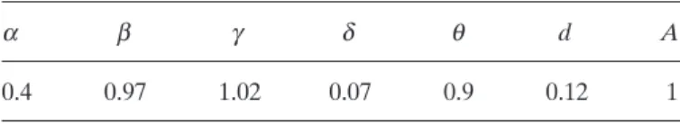
The benchmark calibration is given by Table 1.

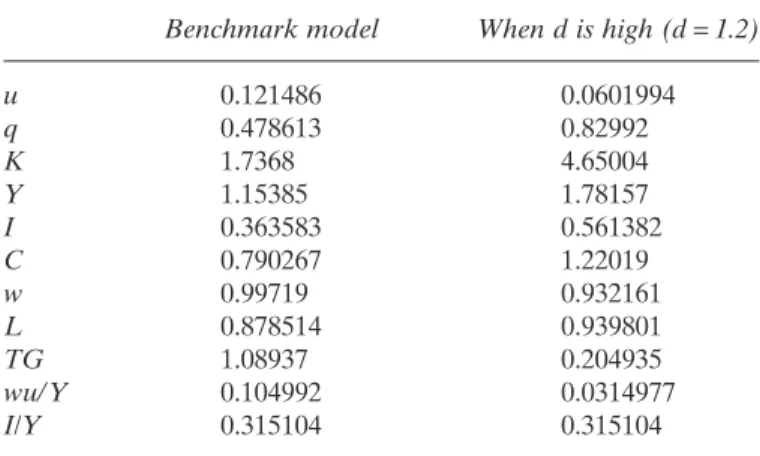
The parameters a, the capital share, b, the time discounting rate, d, the depreciation rate of capital, and A, the level of disembodied technical change, have been fixed to some usual values. For a fixed value of d, the remaining parameters g, the rate of embodied technical change, and q, the “elasticity” of labor in the imitation technology, have been chosen so as to have share of consumption in GDP around 70%, and an adoption cost, as measured by the ratio “wages paid to the technology sector” to GDP, around 10% in the benchmark case. The latter reference value has been given by Jovanovic (1997). In order to illustrate the importance of the institutional and policy aspects, we additionally consider another calibration which only differs from the benchmark in the value of d. Concretely, we consider the case where d equals ten times the benchmark value. Table 2 gives the long-term properties of the two parameterizations.

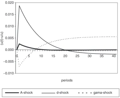
When the economy benefits from policy and institutional environment favorable to technology adoption, the optimal amount of labor resources allocated to the latter activity need not be large, and actually, it is shown to be lower relatively to the bench-mark case. This allows to increase (detrended) output, consumption and investment, without worsening the technological gap, which indeed decreases markedly. These properties reflect the comparative statics demonstrated in Proposition 3. We now turn to the short-term dynamics. We consider three permanent and unexpected 1% shocks affecting the economy from t= 0: a shock on the rate of embodied technical progress, g ; a shock of d and a shock on the level of disembodied technical progress A. The solu-tion paths are given in Figures 1 to 6. Each solusolu-tion path represents the evolusolu-tion of the percentage deviation of a given variable with respect to the initial steady state value.

Before moving to the results of the announced numerical experiments, one should mention that for each shock, the obtained solution path is the unique optimal path.

Table 1. The Benchmark Parameterization

a b g d q d A

First of all, all the considered stationary equilibria are locally saddle-point in the sense of Blanchard–Kahn (1980), that is the set of eigenvalues computed for each station-ary equilibrium is composed of as many eigenvalues as non-redundant (or indepen-dent) forward non-predetermined variables in the linearized model.5_{For example, in} the benchmark model, we find that the linearized model (around the steady state) shows up 2 eigenvalues with modulus larger than one (the highest equal to 1.168) for two independent forward variables and two redundancies. So the Blanchard–Kahn conditions for a saddle-point equilibrium are met, and we find indeed the same local spectral configuration for all the considered stationary equilibria.6

Second, by a Hartman–Grobman like theorem, the saddle-point property is kept in a neighborhood of the considered equilibria, and since we only consider small shocks in our experiments, we are unlikely to break down this property. To be sure about that, we run some sensitivity tests, and it turns out that the solution paths are robust to changes in the experimental parameters.7_{Hence, for each experiment, the computed} path is unique stable.

Optimal Adoption under Technological Acceleration

We first analyze how the economy reacts to the g and the A shocks, as reflected in Figures 1 to 3 for the benchmark case. The main lessons to be drawn from the experiments are:

(i) A technological acceleration through g does not induce an intensification of the adoption effort in the short run. Instead, the optimal amount of labor devoted to the technology sector is below the initial steady state value for around eight periods after the shock. Since the technological acceleration is permanent, the economy will converge to a higher adoption labor long-run value (by Proposition 3). Hence, it has to increase its adoption effort after a while. Whether it does so soon or late depends, in particular, on the settlement of the intertemporal arbitrages and resource competi-tion problems present in the model. Among other relevant factors, time discounting or impatience induces a short-run decrease in labor adoption so as to increase labor in production, which in turn would increase consumption in the short run.

Another important factor is the chosen pattern for the rate of decline of the rela-tive price of capital. In the long run, this rate goes up, involving a change in the composition of output, favorable to investment. So the long-run equilibrium is

un-Table 2. The Long-term Implications of the Calibration

Benchmark model When d is high (d= 1.2)

u 0.121486 0.0601994 q 0.478613 0.82992 K 1.7368 4.65004 Y 1.15385 1.78157 I 0.363583 0.561382 C 0.790267 1.22019 w 0.99719 0.932161 L 0.878514 0.939801 TG 1.08937 0.204935 wu/ Y 0.104992 0.0314977 I/Y 0.315104 0.315104

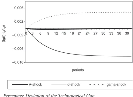
favorable to consumption for two main reasons: a higher adoption labor and a bigger investment rate. In such a context, an optimal reaction in the short run, given the dis-counted nature of the objective function, implies more production labor and/or a lower investment rate. In Figures 1 and 3, we see that while the adoption labor goes clearly down in the short run, there is a very slight increase in the investment rate at t= 1, immediately followed by a long transition below the initial steady state value. By choosing such a behavior, the economy lets the technological gap increase from t= 0 (to the new steady state value). Not surprisingly, welfare maximization does not produce a decreasing pattern for the technological gap, neither in the long run (as proved in Proposition 3), nor in the short run.

(ii) The A shock produces much trickier outcomes. Figures 1 to 3 show a slight increase in the adoption effort, an almost immobile technological gap and a sharp rise in the investment rate, in the short run. It seems that the shock is almost entirely absorbed by the quantity variables, even in the short run! We know by Proposition 4 that only these variables are affected in the long run. Whether the obtained short-run dynamics are robust to changes in the environment (notably to the value of d) is an interesting issue that will be tackled in the next sub-section. Yet it is important to understand why a shock on the level of disembodied technical progress can produce the results we have obtained in the benchmark case.

Notice that such a shock raises the marginal productivity of both production factors, labor and capital. So, it tends to increase both. Now, one should recall that the capital stock (in efficiency units) can be raised either by investing more in the capital sector (which is detrimental to consumption) or by increasing the efficiency level of the new capital goods, which in turn consists in increasing adoption labor since g is fixed. The latter strategy would be attractive if the technology sector could ensure a gain in the efficiency of capital goods (i.e., a rise in q) big enough to compensate the induced labor allocation unfavorable to the production labor in a context of rising marginal

−0.010 −0.005 0.000 0.005 0.010 0.015 0.020 0 5 10 15 20 25 30 35 40 periods (u(t)-u/u)

A-shock d-shock gama-shock

productivity of labor. If not, the adjustment will mainly take place via the quantity vari-ables. This is exactly what happens in our benchmark case. Output, consumption and investment rise. However, the increment in output (and in consumption) is markedly lower than the increment in investment, which is far from surprising since for example production labor slightly decreases. Consequently, the investment rate sharply rises at t= 1. Finally, the resulting technological gap is almost constant over time because of the very limited scope of the reallocation of labor resources. Again, the technological acceleration does not produce any short-term intense adoption effort. However, in

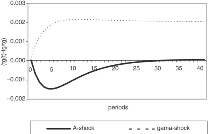
con-−0.010 −0.006 −0.002 0.002 0.006 0 3 6 9 12 15 18 21 24 27 30 33 36 39 periods (tg(t)-tg/tg)

A-shock d-shock gama-shock

Figure 2. Percentage Deviation of the Technological Gap

−0.005 −0.003 −0.001 0.001 0.003 0.005 0.007 0.009 0 5 10 15 20 25 30 35 40 periods (ir (t)-ir/ir)

A-shock d-shock gama-shock

trast to the acceleration in the rate of embodied technical change, the response of the economy is now characterized by an investment boom in the short run.

Institutions, Policy and Optimal Adoption

We now study the robustness of the results listed above to changes in the policy vari-able d. This is done in two steps.

(i) Figures 1 to 3 also report the results of a permanent shock on d for the bench-mark economy. From Proposition 3, we know that the economy will converge to a lower adoption labor, but will achieve a smaller technological gap. So in the long run, labor allocation is favorable to the production sector, and to consumption. In the short run, the economy takes advantage of the improvement in education and/or trade policy and institutions by sharply raising adoption labor. So, in contrast to the case of tech-nological accelerations, institutional and policy improvements in the technology sector can carry out a massive adoption effort in the short run. Note however, that the subsequent decrease in production labor does not lead to a drastic cut in the con-sumption level. Indeed, at the same time, the optimal allocation of the final good is detrimental to the capital sector (see Figure 3).

(ii) In a last experiment, we study the response of the economy to technological accelerations for a value of d, ten times bigger than in the benchmark case. The results are reported in Figures 4 to 6. In the case of the g shock, we get no massive and im-mediate adoption effort after the acceleration, exactly as in the benchmark case. There are, however, some clear quantitative differences. First of all, the initial drop in the adoption effort is less sharp and it takes only four periods to the economy to get above the initial steady state value (it takes eight periods in the benchmark case). Hence,

−0.008 −0.006 −0.004 −0.002 0.000 0.002 0.004 0.006 0.008 0.010 10 5 0 15 20 25 30 35 40 periods (u(t)-u/u) A-shock gama-shock

under better institutions and policy for monitoring technology adoption, the intense phase of adoption starts much earlier, and it converges to a higher adoption labor value and to a lower technological gap (in percentage change with respect to the steady state value).

In the case of the A shock, the differences with respect to the benchmark case are not only quantitative. Recall that such a shock induces an increase in the capital stock which can be achieved either by investing more in the capital sector or by increasing adoption labor. Recall also that the latter is an attractive decision if the technology sector could ensure a gain in the efficiency of capital big enough to compensate the

0.003 0.002 0.001 0.000 −0.001 −0.002 10 5 0 15 20 25 30 35 40 periods (tg(t)-tg/tg) A-shock gama-shock

Figure 5. Percentage Deviation of the Technological Gap when d is High

0.010 0.008 0.006 0.004 0.002 0.000 −0.002 0 5 10 15 20 25 30 35 40 periods (ir(t)-ir/ir) A-shock gama-shock

induced drop in the production labor. In the benchmark case, this condition fails to hold. In the case of large d values, it holds. As a consequence, both adoption labor and the investment rate are boosted in the short run. The pattern of adoption labor induces a decrease in the technological gap in the short run. This is the unique case we find for early and intense adoption efforts, as a response to technological accelerations. Note that this case only concerns the level of disembodied technical progress, and more importantly, it is generated for d values large enough. That is to say the state of policy and institutions around the technology sector is absolutely crucial in the design of optimal technology adoption schedules.

4. Concluding Remarks

Using a simple three-sector model with embodied technical progress, scarce skilled labor resources and a limited capacity of technological absorption, we study the optimal timing of technology adoption. Our main result is the sub-optimality of an immediate increase in the adoption effort in response to an acceleration in the pace of embodied technical progress. The phase of intense adoption (as measured by the share of labor resources devoted to this activity) should be delayed, the exact optimal timing depending on the education and trade policies and institutions at work in the technology sector. In the context of the digital divide debate, our model implies that the latter should not be on the top of any program of economic development (abstract-ing away from the connectivity issue). The specific nature of the technological progress conveyed by the ICT and the weakness of the technology sectors in the South makes this debate irrelevant in our view.

Regarding the globalization debate, our model displays some simple, but useful lessons. The structure of the imitation sector is key in the performances of the devel-oping country, both in terms of long-term income and technological gap. A low productivity imitation sector is a strong signal that the economy will end with a low income and large technological gap in the long run. Since the productivity of the imitation sector strongly depends on the accessibility to the best technologies, global-ization is good if it triggers accessibility to these technologies. However, our model shows that for a fixed imitation sector, there exists an optimal pace of technology trans-fer. Massive and immediate technology adoption is hardly optimal, and this makes the case against the proponents of a globalization abstracting away from the local con-ditions of the national economies.

Appendix

Proof of Proposition 2

By means of successive substitutions, one can reduce the system of eight equilibrium restrictions to a single implicit equation involving only u:

It could be easily checked that G(u) is an increasing and convex function with    

( )

=

[

(

+

)

−

]

−

(

)

− −

(

)

− −

(

)

−

(

)

−

(

−

)

=     − − G u du u u 1 1 1 1 1 1 0 1 1 1 1 q a a g b aq g g d a g b d .

Thus there exists a unique u*∈(0, 1) which satisfies G(u) = 0. Proof of Proposition 3

The comparative statics are derived explicitly. For sake of simplicity, let’s denote by

We have:

It is clear that the denominator is always negative for all values of u. The sign of the expression depends on (u(1+ duq_{)/(1− u) − M). And ∀u, such that G(u) = 0,} (u(1+ duq_{)/(1− u) − M) < 0. Thus, (∂u/∂g) > 0.}

The sign of the expression depends on:

For sake of simplicity, without loss of generality, let d= 1. Then, we have:

so that (∂TG/∂γ) > 0.

The rest of the comparative statics analysis is straightforward: ∂ ∂ g b g q q q u d u u du u =

(

−

)

−

(

+

(

+ −

(

)

)

)

[

]

< + 1 1 1 1 0 1 −

(

−

)

− − −

(

)

(

− −

)

+

(

)

−    −

(

−

)

< + aq g a gq b g b aq q q q 1 1 1 1 1 1 1 0 1 u du du du u , u du u u u du u M b g q q g gq q −

(

+

(

+ −

(

)

)

)

[

]

− −

(

)

(

−

)

(

+

)

− −    1 1 1 1 1 1 1 2 . ∂ ∂g g g gq b g q q q q TG du u u du u M u du u = −

(

−

)

(

−

)

(

(

+

)

(

−

)

−

)

−

(

+

(

+ −

(

)

)

)

[

]

       > 1 1 1 1 1 1 1 1 1 0 2 2 . ∂ ∂g b g q q q u u u du u M du u =

(

−

)

(

(

+

)

(

−

)

−

)

−

(

+

(

+ −

(

)

)

)

[

]

> 1 1 1 1 1 1 0 2 . M R Z R =

(

−

)

(

−

)

(

−

)

−

(

)

+

(

−

)

> − aq g d b g a g aq a a 1 1 1 1 1 0 1 1 2 .     = − − −

(

)

> Z g a d 1 1 _{1 0, and}     = − −

(

−

)

> R g a b d 1 1 _{1 0,} lim , , , . u→1G u

( )

= +∞ asg>1 b<1d>0    

( )

= −

(

−

)

− −

(

)

−

(

)

−

(

−

)

<     → − − lim u 0G u 1 1 1 1 1 1 1 1 0 aq g g d a g b d a a

Since , we get:

and

Proof of Proposition 4

The proof is trivial. Indeed:∂x/∂A= (x/A)[1/(1 − a)] > 0, where x stands for K, C, Y and I. Moreover, from the explicit expression of s given just above,∂s/∂A= 0.

The Stationarized Dynamic System

References

Blanchard, Olivier J. and Charles M. Kahn, “The Solution of Linear Difference Models under Rational Expectations,” Econometrica 48 (1980):1305–13.

˜ _{˜ .} Lt+ =1ut ˜ ˜ ˜ Ct+ − = 0It Yt ˜ ˜ ˜ ˜ Yt=A K Lt ta 1t−a ˜ _{˜ ˜} ˜ Kt=q It t+ −

(

)

Kt− t − − 1 1 1 1 d g a ˜ ˜ ˜ ˜ ˜ qtgt =qt−1+d ut tqgt

(

1−qt

)

1−

(

_a

)

˜ ˜a ˜−a ₌ ˜ ˜ A K L C w t t t t t ˜ ˜ ˜ ˜ ˜ ˜ ˜ ˜ ˜ ˜ ˜ ˜ _{˜ ˜} K K q C d u w d u q w d u q t t t t t t t t t t t t t t t t − −

(

)

₌

(

+

)

−

(

)

−

(

−

)

− − − − + + + +− + 1 1 1 1 1 1 1 2 1 1 1 1 11 1 d g q b g q a q q q ˜ ˜ ˜ ˜ ˜ ˜ ˜ ˜ C C q q q A K L t t t t t t t t t + + ++ − − = −

(

)

[

−

]

1 1 1 1 1 1 1 1 1 g b d a a a a ∂ ∂ s d= 0.         = −

(

−

)

(

−

)

−

(

)

−

(

−

)

− −

(

)

−

(

−

)

>    − − − − − 1 1 2 1 2 ₁1 2 1 1 1 1 1 1 1 1 1 1 0 a a a a a a ∂ ∂g a b g g a g b d g d g b d s ,         = = − −

(

)

−

(

−

)

− − − a a a a a g d g b d 1 1 1 1 1 1 1 s I Y ∂ ∂ g g b g b g q q q q TG d u du d du u =

(

−

)

[

(

+

)

−

]

−

(

+

(

+ −

(

)

)

)

[

]

< − 1 1 1 1 1 0 2 .

Boucekkine, Raouf, “An Alternative Methodology for Solving Nonlinear Forward-Looking Models,” Journal of Economic Dynamics and Control 19 (1995):711–34.

Boucekkine, Raouf, Fernando del Río, and Omar Licandro, “Embodied Technological Change, Learning and the Productivity Slowdown,” The Scandinavian Journal of Economics 105 (2003):87–98.

Dinopulos, Elias and Paul S. Segerstrom, “A Theory of Globalization,” Manuscript. Stockholm School of Economics (2003).

Gordon, Robert J., “Does the New Economy Measure up to the Great Inventions of the Past?”

Journal of Economic Perspectives 14 (2000):49–74.

Greenwood, Jeremy, Zvi Hercowitz, and Per Krusell, “Long-Run Implications of Investment-Specific Technological Change,” American Economic Review 87 (1997):342–62.

Greenwood, Jeremy and Yorukoglu, Mehmet, “1974,” Carnegie–Rochester Conference Series on

Public Policy 46 (1997):49–95.

Grether, Jean-Marie, “Determinants of Technological Diffusion in Mexican Manufacturing: a Plant-Level Analysis,” World Development 27 (1999):1287–98.

Jovanovic, Boyan, “Learning and Growth,” Advances in Economics, London: Cambridge University Press, 1997 (Vol. 2).

Juillard, Michel, “DYNARE, a Program for the Resolution of Nonlinear Models with Forward-Looking Variables. Release 2.1,” CEPREMAP, Working Paper 9602 (1996).

Nelson, Richard R. and Edmund S. Phelps, “Investment in Humans, Technology Diffusion and Economic Growth,” American Economic Review 56 (1966):69–75.

Niosi, Jorge, Petr Hanel, and Liette Fiset, “Technology Transfer to Developing Countries through Engineering Firms: the Canadian Experience,” World Development 23 (1995):1815–24. Segerstrom, Paul S., “Naomi Klein and the Anti-Globalization Movement,” Manuscript.

Stockholm School of Economics (2003).

Wacziarg, Romain T. and Karen Horn Welch, “Trade Liberalization and Economic Growth: New Evidence,” Manuscript. Stanford University (2002).

Notes

1. See the excellent work of Grether, 1999, on the Mexican case. 2. French inter-ministerial committee, July 10, 2002.

3. Since we are considering optimality issues, this is by no way a limitation. We could have con-sidered a decentralized set-up à la Dinopoulos and Segerstrom (2003), but the computation of the short-term dynamics is so problematic in the latter case that we turn to an optimal growth framework to make our point.

4. We use Dynare, the package developed by Juillard (1996), for the simulation and stability assessment of nonlinear forward-looking variables.

5. The computation of the eigenvalues requires a state-space representation, called the Blanchard–Kahn form, which is not generally directly available from the structural model, due to collinearity inducing non-invertibility of matrices. Redundancies should be removed, and that is exactly what Juillard’s software, Dynare does.

6. However, there is no way to establish this property analytically given that we don’t have closed-form stationary equilibria, and more specifically, because the analytical obtention of the Blanchard–Kahn form—namely the removal of redundancies—is impossible.

7. For an extensive and mathematically founded exposition of these sensitivity tests in the context of Newton–Raphson relaxation algorithms as the software Dynare, see Boucekkine (1995).