A continuous review inventory system in a random environment

H P S - ^ S Z • S S

JS 2 3

/ааѳ

л

mïïwmmz шмш

ш і ш

íh

...

A CONTINUOUS REVIEW INVENTORY SYSTEM

A RANDOM ENVIRONMENT

A THESIS

SUBMITTED TO THE DEPARTMENT OF MANAGEMENT AND THE GRADUATE SCHOOL OF BUSINESS ADMINISTRATION

OF BILKENT UNIVERSITY

IN PARTIAL FULFILLMENT OF THE REQUIREMENTS FOR THE DEGREE OF

MASTER OF SCIENCE

By

Asli Bayar

25 09 1998

ί1{

R ч я

I certify that I have read this thesis and that in my opinion it is fully adequate, in scope and in quality, as a dissertation for the degree of Master of Science.

i.ssist. Prof. Emre Berk (Supervisor) I certify that I have read this thesis and that in my opinion it is fully adequate, in scope and in quality, as a dissertation for the degree of Master of Science.

_________ j p

Assoc. Prof. Erdal Erel

I certify that I have read this thesis and that in my opinion it is fully adequate, in scope and in quality, as a dissertation for the degree of Master of Science.

Approved for the Graduate School of Business .Adminis­ tration;

L I A J o .

Prof. Dr. <^bmey

A b str a c t

A CONTINUOUS REVIEW INVENTORY SYSTEM IN A

RANDOM ENVIRONMENT

Aslı Bayar

M. S. in Management

Supervisor: Assist. Prof. Emre Berk

25 09 1998

In this thesis, we develop a continuous review inventory model in a random environment where holding, ordering, and purchasing cost parameters are dependent on the state of the environment. We derive the exact expressions of the operating characteristics of the model and discuss some convexity properties of the expected cost rate. A numerical analysis is provided to examine the sensitivity of the optimal policy parameters with respect to various system parameters. We compare the instantaneous shock model with our model and illustrate that ignoring finite duration of environmental states results in considerable error. Moreo\er. we compare our model with a time-average EOQ and myopic model. The results illustrate that when ordering and purchasing cost parameters change, our model performs significantly better.

ö z e t

d e ğ i ş e n b i r o r t a m d a s ü r e k l i g ö z d e n

GEÇİRİLEN

BİR STOK KONTROL SİSTEMİ

Aslı Bayar

İşletme Yüksek Lisans

Tez Yöneticisi: Assist. Prof. Emre Berk

1998

Bu tezde stokta tutma, sipariş ve satın alma maliyet parametrelerinin dış çevre durumuna bağlı olduğu değişken bir ortamda sürekli gözden geçirilen bir stok kontrol modeli geliştirdik. Modelin işletim özelliklerinin kesin ifadeleri ve beklenen maliyet oranının bazı konvekslik özellikleri saptandı. En iyi politika parametrelerinin çeşitli sistem parametrelerine karşı hassasiyetini incelemek için sayısal bir analiz yapıldı. Anlık .şok modeli ile geliştirilen model karşılaştırıldı ve dış çevre durumlarının sürelerini gözardı etmenin dikkate değer bir hata yarattığı gözlemlendi. Ayrıca, geliştirilen model, uzun zaman ortalamalı ekonomik sipariş miktari modeli ve niiyopik bir modelle karşılaştırıldı. Sayısal çalişma sipariş ve satın alma maliyeti parametrelerinin değiştiği ortamlarda geliştirilen modelin diğer politikalara kıyasla daha iyi sonuç verdiğini ortaya çıkardı.

To ту family

A ck n ow led gem en t

I want to thank to my family first, for their continuous support during the preperation of thesis and throughout my life.

Special thanks to my thesis supervisor Assistant Prof. Dr. Emre Berk for his guidance throughout this study.

C o n ten ts

A bstract j

Özet jj

A cknowledgem ent iv

Contents V

List of Figures vii

List of Tables viii

1 Introduction 1

2 Literature R eview 4

3 M odel 9

3.1 Derivation of the Model 9

3.1.1 Case I ... 12 3.1.2 Case I I ... 14 3.1.3 C a s e i n ... 15 3.2 Derivation of the Cost F u n c tio n ... Ig

3.2.1 Cost Functions for Case I 17

3.2.2 Cost Functions for Case I I ... 3q

3.3.1 Case I ... 36

3.3.2 Case I I ... 37

3.4 Conve.xity of the Total Cost R a t e ... 38

4 Num erical R esults 46 4.1 Parameter S e t ... 46

4.2 Sensitivity Results ... 47

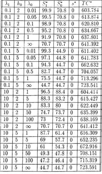
4.2.1 Sensitivity Results for /i q... 47

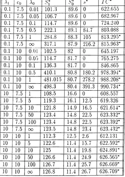
4.2.2 Sensitivity Results for Cq ... 48

4.2.3 Sensitivity Results for k o ... 48

4.3 Comparison With Instantaneous Shock M o d e l... 49

4.3.1 Comparison of the Models When ho Changes... 49

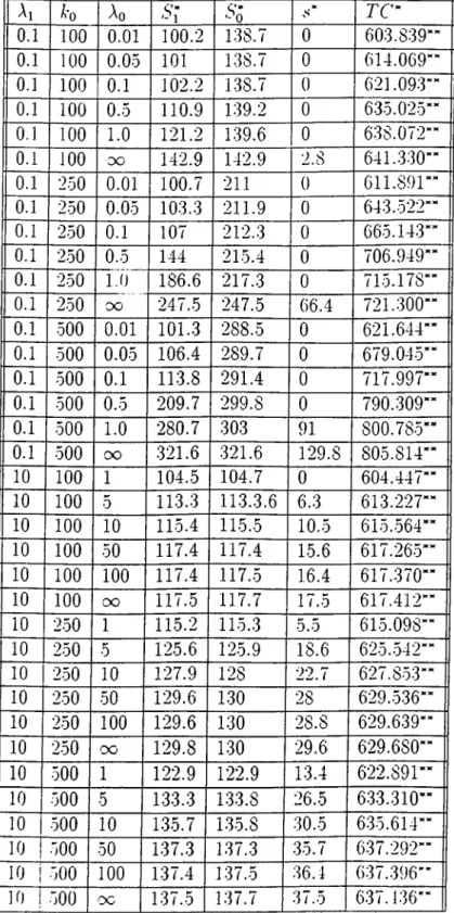
4.3.2 Comparison of the Models When cq C hanges... 50

4.3.3 Comparison of the Models When ko Changes... 50

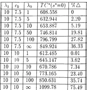
4.4 Optimal Total Cost per Unit Time When ..s'= 0 ... 51

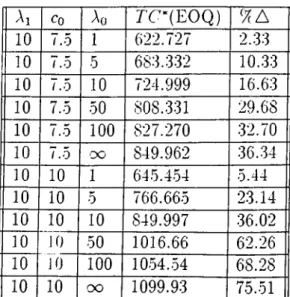
4.5 Numerical Comparison With A Time-Average EOQ Model . . . . 52

5 Conclusion 61 A P P E N D IX 63 A.l Appendix A ... 63

A.1.1 Derivation of Conditional P ro b ab ilities... 63

List o f F ig u res

3.1 Case 1...43 3.2 Case II...44 3.3 C a se in ...45

List o f T ables

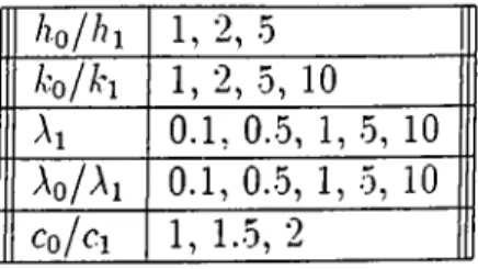
4.1 Parameter.^ Set Used in the Sensitivity A n a ly sis... 46

4.2 Sensitivity Results for / i o ... .53

4.3 Sensitivity Results for cq... 54

4.4 Sensitivity Results for ko... 5.5 4.5 Behavior of Optimal Values with Respect to Tested Cost Parameters 56 4.6 Comparison of the Models When ho Changes... 56

4.7 Comparison of the Models When cq C h an g es... 57

4.S Comparison of the Models When ko C hanges... 58

4.9 Comparison of the Results When cq Changes and ¿¡’“= 0 ... 59

4.10 Comparison of the Results When ko Changes and .s* = 0 ... 59 4.11 Comparison with Time-Average EOQ When cq Changes 60

4.12 Comparison with Time-Average EOQ When ^^0 Changes 60

C h ap ter 1

In tro d u ctio n

In the real world, big economic crises can be observed, like the ones in 1929 in the USA, in 1994 in Turkey, and Mexico, in 1997 in Asia, and in 1998 Russia. In such crises, environmental conditions may change very frequently in a random manner, and big volatilities can be observed in some economic variables, such as GNP, interest rate, exchange rates, and demand rates.

In an economic crisis, inventory management is one of the areas, which are affected from the changes in the environmental state. In inventory management, all of the cost parameters depend on the state of the environment at a point in time. Depending on the changes in the environmental state, purchasing price of the item, fixed ordering cost, holding cost, demand rate, and supply conditions may change separately or together.

Weather conditions, shortages, or political crisis can create randomness in the supply conditions and they may lead to random lead time. Moreover, the demand for many products responds in part to changes in certain basic economic variables, such as GNP, or interest rate. For instance except for .some cheap products such as bread, as the G.NP increases the demand for tlie product increases. However, as interest rates increase, borrowing becomes more expensive, so the demand for the product declines. I he demand for the product changes also depending on shifts in consumer tastes.

Changes in the interest rates in the financial environment affect the holding

Chapter 1. [ntroduction

cost in inventory luanagement. When the interest rates are high, if a firm holds large amount of inventory on hand, (since it can not earn interest from the inventory on hand), it gives up the interest it would earn if it made investment in financial instruments. So, depending on the changes in the interest rates, holding cost in the inventory management changes.

The price of the item is affected from the changes in inflation rate and the random deal offerings of the suppliers. For the imported items, changes in the exchange rate affect the price of items. When the exchange rate increases, the purchasing price of the item increases.

In the literature under periodic review assumption for a single product, there are many studies in which all the cost parameters change depending on the changes in the environmental conditions. However, under the continuous review, the focus of research has been on the case where there is a price increa.se/decrease at an announced time. Among the studies in this area, only Moinzadeh[1.5](1997), considers an inventory system in which the product can always be procured at the list price and at random points in time price discounts are offered to the system by the market or the supplier(s) at a reduced price. The study assumes that the price discounts have no duration (i.e., is instantaneous)

In this study, we consider a continuous review inventory system for a single product where the holding, ordering, and purchasing cost parameters change in a random manner. In the system, there are two environmental conditions called state 0. and state 1. and the frequency of occurrence of these states follows exponential distribution. However, unlike in Moinzadeh[15](1997), in our study state 1 is not instantaneous.

Under the assumptions of no backorder, and negligible lead time, using optimal three parameter (5i,5'o,s) type inventory management policy, we derive the exact expressions of the key operating characteristics of the systerii for the deterministic demand.

Even though the main application area of this study is inventory management, it is also possible to use the considered model in cash management. In such an application, instead of determining the optimum amount of inventory on hand.

Cluiptcr 1. Introduction

the optimum amount of money an individual can keep in his pocket is determined. This thesis co\crs the following chapters. In Chapter 2, we present the literature on a single product under both the periodic and continuous review inventory systems in a changing environment.

In Chapter 3, we explain the three parameter optimal policy, and derive the key operating characteristics of the model. Expected total costs per unit time both when the holding cost is constant and changing, are calculated. And under some assumptions conve.xity of the total cost per unit time in some key inventory parameters are illustrated.

In Chapter 4, we present our numerical results on a wide range of parameter settings. .Since the total cost expression is very complex, it can not be possible to derive analytical optimum results for the system.. We make sensitivity analysis, for the expected total cost per unit time with respect to changes in the values of holding cost, ordering cost, purchasing cost, frequency of occurrence of state 0, and frequency of occurrence of state 1.

In chapter 5, we conclude the thesis by summarising our findings, and possible future researches.

C h ap ter 2

L iteratu re R ev iew

In this chapter, we present the previous work on inventory systems in random environments. The models developed for the random environment can be classified into two groups, as periodic review inventory models, and the continuous review inventory models.

The earliest study on random environment inventory system is Hunter, and Kaminsky[10](1968). In their work, an inventory control model is developed for an environment in which random opportunities for reduced cost replenishments occur. Both demand, and the opportunities for special reduced- cost replenishment come from Poisson processes. Order lead time is negligible. A three-parameter (5'i,-^2i'5'2) ordering policy is proposed. Under this policy , an order of size ,5'i is placed at the regular price as the inventory is depleted. When a special opportunity for reduced unit cost occurs, given that inventory level is less than ¿ 2, an order is made to raise the inventory level to S2· In their analysis,

they consider two separate cases, L2>S\, and S'i>L2· As a solution they suggest

a three dimensional search on the three control parameters, 5'i, ¿ 2, and S2.

Kalymon[ll](I971) studies a multi-period inventory model in which future prices of the purchased items are determined by a Markov stochastic process. It is assumed that inventory decisions are made at regular intervals. The inventory level is known at the beginning of each period, and the current price is known before purchases are made. Inventory levels are depleted by demand which in

Chapter 2. Literature Review

each period is a random variable whose probability distribution may depend on the current price. The paper proves the optimality of policy in the finite horizon case.

In Golabi[6]( 1985). a single item inventory control model is developed in an environment in which ordering price is randomly distributed according to a known distribution function. Demand is constant. Backlogging is not allowed. At the beginning of each period, a random ordering price is received according to a known distribution function. The objective of the study is identified as the calculation of the optimal order quantities in each period which satisfying all demands, minimizes the total expected cost. The main result of Golabi[6](1985) implies that at the beginning of any period, the firm must order an amount to satisfy the demand.

Song and Zipkin[23](1991) derive an inventory model, in which the demand rate varies with an underlying state of the world variable. The world is modeled as a continuous time Markov chain. In the model, when the world is in the state k, demand follows a Poisson process with rate A*,.. There is an order lead time, either fixed or stochastic. The main results of the paper are that if the order cost is linear in the quantity ordered, base-stock policy is optimal. On the other hand if there is also a fixed cost to place an order, a state-dependent (r,S) policy is optimal, in which r is the reorder point, S is the order-up-to level.

Silver, Robb, and Rahnama[21] (1993) consider the same problem with Hunter and Kaminsky[10] (1968). However, they make the assumption that L-2>Si. They

then develop an approximate solution method which is much easier to use. They do not consider the condition that S i > L2, because occurrence of a fairly large

fixed cost for each special replenishment is very unlikely, there is a small difference in the unit cost of the material between regular and special replenishments, and very frequent opportunity for special replenishments do not occur in the real world.

Ozekici, and Parlar[17]( 1997) provide an infinite-horizon periodic-review inventory model in a random environment where the supply, demand, and cost parameters may change instantaneously. The state of the environment is

Cliaptcr 2. Litcvdturc Review

ck'sn ibed by a Markov chain. There i.s complete backlogging of the demand. In tlu' study, they .show that an environment dependent order-up-to level policy is optimal when the order cost is linear in order cpumtity. When there is also a fi.xed cost of ordering, it is shown that a two-parameter environment dependent (si.S'i) policy is optimal under some specific conditions.

Finally, in the periodic review literature, we should mention Hall[9](1992) who compares the cost rate model, and the present value model in an environment in which from time to time, the unit-purchasing price of the good may change in discrete steps. In both models, there is no order lead time and demand is constant. In the study, comparison of these two approaches reveals that when the price reduction is more than 40 percent, present value approach is more preferred, since in the present value approach the cost of holding inventory is not undervalued.

Under the continuous review, the main focus of research has been on the case where there is a price increase/decrease at an announced time.

.Among the continuous review inventory management models, Taylor, and Bradley[27] (1985), develop optimal ordering policies for an environment where the announced price increase becomes effective at any future specified time rather than at the end of economic order quantity cycle.

.Ardalan[l](19SS) analyses the effects of a special order on inventory cost when a supplier reduces the price of a product temporarily, and develops an EOQ-type optimal policy in response to a sale. The paper assumes that the sale period is short relative to the regular inventory cycle, and it is not required that reduced price is in effect at the replenishment time. In the model, the total holding and ordering costs may also be affected by size, and time of special order.

Lev and Weiss[12](1990), relaxing the basic assumptions of the classical EOQ inventory model (infinite time horizon, and static costs), develop models for finite and infinite-time horizon optimal inventory policies in a random environment in which all or any costs change. In the model, there is no order lead time, holding cost is fixed, and at the beginning the time of the price change is announced. They show that all orders placed before the time of the last opportunity to purchase

Chapter 2. Literature Review

at low price are of the same size, and all orders placed after the time of the last opportunity are of the same size.

Recently, Moinzadeh[15](1997) analized an inventory system where price discounts are offered at random points in time, which are e.xponentially distributed. In the model, demand is assumed constant, order lead time is assumed to be negligible and no backorders are allowed. The discount (deal) itself have no duration (i.e. is instantaneous). In the model a three parameter (,S'i, So, s) control policy is employed, and its convexity properties which are imitates of EOQ-type approximations to some polic}· parameters are also provided.

We should also mention the work on supply conditions. Parlar and Berkin[18](1991) deal with a continuous review inventory model where supply availability is a random variable. It is assumed that during a ”wet” period supply · is available in any amount that is desired, whereas during a ’’dry” period, it is impossible to obtain any supply. The demand that is not satisfied during a dry period is lost. Under an EOQ type ordering policy, the system is analyzed.

Berk, and Arreola-Risa[‘2](1994), build their study on Parlar and BerkinflS] (1991) and remove an implicit assumption in their work.

Parlar and Perry[19](1995) consider a stochastic inventory model where supply conditions (lead times) are random due to some factors such as strikes. In the study, the supplier's availability process is represented as a two-state continuous time Markov Chain where one state corresponds to availability (ON), and the other state corresponds to unavailability of the supplier (OFF). They assume that if the order arrives, the state is identified as ON, and in this state lead time is zero. The duration of both the ON state and the OFF state are exponentially distributed. In the model, to make an order the firm does not have to wait until the inventory level reaches zero, reorder point is defined as one of the decision variables. They use (S, s) type inventory policy. The paper identifying the objective function as the long-run average cost, determines the optimal v'alues for the reorder point, the order cjuantity when the system is in ON state, and how long to wait before the next order if the system is OFF state.

Chapter 2. Literature Review

ill a random environment in which supply availibility is subject to random fluctuations. In the system, there are two suppliers, and their availability may be individually either ON or OFF. They assume that the duration of the ON periods for the two suppliers are distributed as Erlang random variables, and the OFF periods for each supplier have a general distribution. They use (S, s) type policy, and define their objective as minimization of long-run average cost.

In our study, we develop a continuous review inventory model in a random environment in which holding, ordering, and purchasing cost parameters change depending on changes in the environment. Among the previous studies, Moinzadeh[lo](1997) is the closest to our model. As in Moinzadeh[lo](1997), we assume that the demand is constant, order lead times are negligible, no backorders are allowed, and the occurrence of state 1, and 0 are poisson process. However, unlike in Moinzadeh[15](1997), in our study state 1 has positive duration, (i.e. is not instantaneous), and thereby holding cost also changes depending on environmental conditions.

C h ap ter 3

M od el

In this chapter, a continuous review inventory model is developed under a three- parameter control policy operating in an environment in which state changes in a random manner. We begin our analysis by stating the assumptions of the model. We then introduce the control policy employed in the model. We derive the expressions for the operating characteristics of the system, and the expected total cost rate. Lastly, we discuss some convexity properties of the cost rate.

3.1

D erivation o f th e M od el

We consider an inventory system under the following assumptions: 1. Demand rate is constant over time, D.

2. The environment in which the system operates can be found in two states. 0 and 1.

3. The time between changes in the state of the environment is random, and is exponentially distributed. The change from state 0 to 1 occurs with rate Ai, and the change from state 1 to 0 occurs with rate Ao .

4. Order lead times are negligible. 5. No backorders are allowed.

Chapter 3. Model 10

6. Holding cost is iiicurrecl at /i, per unit held in stock per unit of time in state i (i=0,l).

7. Each order placed in state i (i=0,l) incurs a fixed ordering cost ki.

8. Purchasing cost is incurred at c,· per unit purchased in state i (i=0,l).

In chapter 5, we discuss how each of the assumptions may be relaxed and what impact they would have on the analysis.

We know from Song and Zipkin[23](1991). and Ozekici and Parlar[17](1997) that the optimal control poli':y class is of a state-dependent (5), Si) type for periodic review inventory systems. In Song and Zipkin[23](1991) (see Theorem 3 in pcige 358), in the case where there is a fixed cost to place an order, it is shown that a world-dependent (r,S) policy is optimal. That is under case of two states, optimal control policy is of four parameter (S'!, ¿¡i. So, .sq). In continuous review

inventory systems, three parameter (5'i, ,S'o, s) inventory control policies would be optimal when the order lead time is negligible. However, when there are order lead times, inclusion of another non-zei’o reorder point is necessary resulting in

{Si, Si) control policies. Under continuous review, Moinzadeh[15](1997) propo,ses

a three-parameter (5'i, So, s) policy without discussion of optimality in the ca.se of two environmental states when there are no order lead times.

In this study, since we assume that there is no order lead time, we consider a state-dependent three-parameter inventory control policy.

The following control policy is empIo\'ed:

POLICY'A) If the inventory level is at or below s when the system is in state

1, the inventory level is raised to ^i;

ii) If the system is in state 0, the inventory level is raised to ,S'o when inventory level drops to zero.

This policy will be referred to as the [Si, So, s) policy. Under this policy, if the inventory level is greater than s, no order is made. An order may also be placed anywhere between s and zero it the environment is found in state 0 at s, and a change in the state from 0 to 1 occurs afterwards. Si and Sq are the

Chapter 3. Model 11

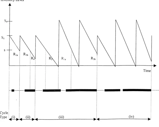
To define a cycle and a regeneration point, we need to know the state of the environment, and the inventory level at the regeneration point, and both of them (the state of the environment and the inventory level j should have the same values at each time the inventory level reaches the regeneration point. In our model, we define a cycle as the time between two consecutive replenishments when the state is 1 ( in other words when the inventory level is raised to 5i). It is also possible to identify the instance when state 0 replenishments occur as a regeneration point. However, it is not possible to identify instance at which inventory level hits s, since at that instance the state may be 0 or 1.

For ease of exposure, we define Qi=Si-s and Qo=S'o-s.

Note that there may be many changes in state from 1 to 0, and 0 to 1 in a cycle. However, only the ones that occur when inventory on hand is less than or ecpial to s affect the ordering decision. Depending on the definition of a cycle, and the possible values. Si, (Q i+s), ^o, (<3o+s), and s may take, there are three possible cases. In case I, S\ is greater than or equal to So, and So is greater than or equal to s, (^i > So > s). In case II, again .Si is greater than or equal to So, but So is less than or equal to s, (¿"i > s > ^o). In case HI, So is greater than or ecjual to Si, and ,S'i is greater or equal to than s. In the model. So > s > Si case is not a realistic case. According to the policy when the inventory level is less than or equal to s level, if state 1 occurs, an order is made to rise the inventory level to Si- However, in that case, since Si is less than or ecjual to s, it is not possible to make an order when the state becomes 1 and the inventory level on hand is between s and ,?i.

For the sake of clarity, it may be assumed that state 1 refers to a discount state, i.e. low cost, and state 0 is a high cost state. When state is 1. if we analyze the system in terms of purchasing cost since the unit purchasing cost is low in state 1, one would want to buy as much as it can at low cost, so 6'i would be greater than So- Also due to high unit purchasing cost So would be chosen as small as possible; in some cases. So might be chosen even smaller than s. Therefore, it is necessary that we consider both case I and case II in the analysis.

Chapter 3. Model ₁₂

If we analyze the system in terms of holding cost, when state is i. since unit h'jlding cost is low. opportunity cost of holding inventory is not high, so to keep large amount of imentory does not cost much. Fle-nce we would consider onlv case I in which ,S'i is greater than or ecjual to ,5'o.

However, if we analyze the system in terms of ordering cost, we see that the optimal policy might happen in both case I, where Qi is greater than or equal to Qi), and case III where Qi is less than or equal to Qo- Both of the cases are considered because as Qi increases, number of units purchased in state 1 increases, and the number of replenishment declines. On the other hand, as optimal Q(j values increases, fixed ordering cost per unit of order declines.

3.1.1

C ase I

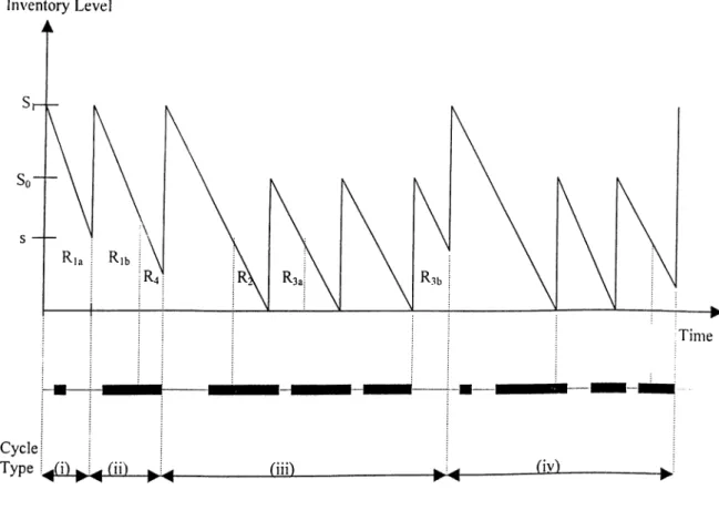
.A.S can be .seen from Figure 3.1, in case I, there are four possible cycle types. The first cycle type starts with inventory level at S\, and environment is in state 1 and until inventory level declines to s, some changes may occur in the environment from state 0 to state 1. But given that state is 1 at the inventory level s, Qi units of inventory is ordered when the inventory level is equal to s. In other words, cycle ends when inventory level hits s, and the state is 1.

The second cycle type starts with an inventory level at 5i and environment is again in state 1 and until inventory level declines to s, environment changes from state 0 to state 1. However, the state is 0 at the inventory level s. and at the inventory level I , which is between s and 0, state changes from 0 to 1. As soon as this change occurs, (5 i-/) units of inventory is ordered. In short, cycle ends when the state becomes 1 at inventory level I .

Unlike in the first, and the second cycle types, in the third, and fourth cycle types there are replenishments when state is 0. These cycle types occur when state 0 goes on for a long duration. The main difference between the third, and fourth cycle types is that unlike in the third cycle type in which state changes from 0 to 1 when the inventory level is greater than s, in the fourth cycle type the state changes from 0 to 1 when the inventory level is below the s.

Chapter 3. Model 13

To calculate the operating characteristics, sonu- rf-gions are defined, and the cycle types are divided into the identified regions calh?d R2,

and III as illustrated in Figure 3.1.

Ria region covers the area between inventory levels ,?i and s. In / 2i,, region,

at the inventory level 5i, environment is in state 1. between inventory levels ,S'i and s state can be 1 or 0, however, it must be 1 when the inventory level falls to s. Ri.i region e.xists in cycle type (i) of case I.

Like Ria region. Rn, region covers the area between inventory levels ,S’i and s. However, in Rib region, at the inventory level ,S'i. state is 1. between inventory levels ,S'i and s state can be 1 or 0, but it must b(.> 0. when the inventory level is equal to s. R u region occurs in cycle type (ii), cycle type (iii), and cycle type (iv) of case I.

Ro region is observed when state 0 goes on for a long duration, and the number

of replenishments when state is 0 is greater than zero. R2 region covers the area between inventory levels s and 0. In that region, the state is always 0. Depending on how long state 0 goes on, it is possible to observe occurrence of R2 region in a cycle type more than once. If state becomes 1 between inventory levels s and 0, a replenishment is made, cycle ends, and R2 region can not occur in that cycle type any more. R2 region takes place in the third and fourth cycle types.

Like region, Rsa region is observed when the number of replenishments when the state is 0 is greater than zero. R^a region covers the area between inventory levels 5'o and s. In R^a region, given that at .S'o inventory level the state is 0, between inventory levels So and s there may be changes from 0 to 1 or 1 to 0 states, and. at s inventory level the state is 0. Since inventory level is above s level, unlike in R2 region, in R^a region such changes in the state of environment do not affect the system. R^a region takes place both in the third and fourth cycle types.

Like Roa region. R-.iij region covers the area between im’entory levels Sq and s and it is observed when the number of replenishments when the state is 0 is greater than zero. In Rob region, at inventory level So the state is 0, it will be 1 at the s inventory level. Unlike Roa region, Rob region occurs only once in cycle

Chapter -i. Model U

type (iv). It does not occur in cycle type (iii).

d'he region between inventory levels s and / is chilled as R.i region. In that region / is the inxentory level at that the state char.ges from 0 to 1; / can take any value between s and 0. In B..i region, until inventory level / is reached, state 0 is observed. At the inventory level /, conditions change from 0 to 1 and at that point [Si-I) units of inventory is ordered. i{\ region takes place only in th(> second and fourth cycle types. In each cycle t\ pe. region does not occur more than once, and when region occurs, the cycle ends. The main difference between R^ region and the other regions is that region is a random region. The length of the region may change depending on the possible values / may take between inventorv levels s and 0.

3.1.2

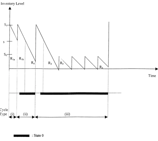
C ase II

In case II, given that S\ is greater than or equal to s, So is less than or equal to s , (,5'i > s > So)· As can be seen from Figure 3.2. , unlike in case I, in ca.se II there are three different cycle types. First, and second cycle types are the same with the first and second cycle types in case I. Like in the first cycle type of case I, in the first cycle type of case II, only R u region occurs. Moreover, like in second cycle type of case I, in the second cycle type of case II, both and i?4 regions take place. However, cycle type (iii) is different from cycle type (iii) in case I. In cycle type (iii) of case II, there are replenishments when the state is 0, and since .S'o value is less than or equal to s value, the replenishment may occur when the inventory level is greater than

So-Like in ca.se I, to make calculation of the total cost, some regions are defined, and the cycle types are divided into the identified regions called, R2. R4, and

Ro-Ria- and Rib regions are the same with the Ro-Ria- and Rn, regions identified in

case I.

R2 region covers the area between inventory levels s and 0. In that region, the state does not change from 0 to 1. Except for the probability (expected number)

r '/ if ip ie r 3. Model 15

of ocruneiice, Ry region is the same with the R2 region in case I. In case II, R2

ro'gion is observed only in the third cycle type.

R- t region covers the area between inventory lev(,‘ls s and I. /, which can take

value between s and 0 inventory levels, is again defined as the inventory level at which state changes from 0 to 1. Unlike in case I. in case II, R4 region occurs only in the second cycle type. Thus except for the probability (expected number) of occurrence, R4 region is the same with the R4 region in case I. Like in case I. in case II, the length of the R4 region changes depending on the possible values / can take between s and 0 inventory levels.

Ro region is observed when replenishments in state 0 occurs. In other words,

it is observed only in the third cycle type. R5 region covers the area between inventory levels So and 0. In that interval, the state is always 0; no state 1 occurs. When state 0 remains for a long duration, R^ region occurs more than once.

The region between inventory levels So and I is called as Rq region. Like R5

region, Ro region is observed only in the third cycle type. In that region I is the inventory level at that environmental conditions changes from 0 to 1. I can take any value between So and 0. In Ro region, until inventory level I is reached state 0 is observed. At inventory level / the state changes from 0 to 1 and at that point (Si-I) units of inventory are ordered. Ro region is also a random region. The length of the Rq region depends on the possible values / can take between .S'o and 0 inventory levels.

3.1.3

C ase III

As can be seen from Figure 3.3. case III is almost the same with case I. Like in case I, in case III, there are four different cycle types, and in those cycles R^a- /?i6, R:ih· ‘'■nil -^4 regions are observed. The main big difference between

case I, and case III is that unlike in case I, in case III ,S'o is greater than or equal to 5'i, (5o > Si > s). E.xcept for restriction that .S’o > ,S'i, case III is the same as case I. Therefore we do not enumerate cycle types, and the regions in this case.

Chapter 3. Model IG

3.2

D erivation o f th e Cost Function

In calculation of the expected total cost function, conditional probabilities identifying the state of the environment are needed. However, our problem is similar to the M /M /1/1 queuing system in which derivation of the transient probabilities that at an arbitrary time t, there are n customers in a single channel system with Poisson input, exponential service, and no waiting room is a straightforward procedure'. In our model, state 0 refers to the condition that there is no customer in the M /M /1/1 queuing system. And state 1 refers to the condition that there is one customer in the M /M /1/1 queuing system.

Using M /M /1/1 queuing system, as explained in the appendix A the following conditional probabilities are calculated:

Pio{t): The probability that the state will 0 at time t given that it is 1 at

time zero.

Poo{i)· The probability that the state will 0 at time t given that it is 0 at

time zero.

Pn(t): The probability that the state will 1 at time t given that it is 1 at

time zero.

Poiit): The probability that the state will 1 at time t given that it is 0 at

time zero.

n o f i j - (,\i+Ao) (3.1)

Poo{i) — _(Ai+Ao) (.3.2)

P ( i \ — Ai+Ane

Pn{t) - (,q+A„) (3.3)

PoM) =_ Ai(l-e~(^i + '^u)')_(-\l+-\o) (3.4) Pi is the probability that the state will be 0 at the inventory level s given that at inventory level 5i it is 1.

Pi = f\o(Qi/D)

Pi - (aTTa^)

P2 is the probability that between inventory levels s and 0 state 1 does not occur. In other words, in the 0- s/D time interval, state 1 is not observed, only state 0 is observed.

P2 = (36)

P'i is used only in case I. It refers the probability that given that at im'entory

level Sq the state is 0, again it will be 0 when the inventory level is equal to s. i^3=Poo(go/D)

Chapter 3. Model 17

■^3 - ( A i + A o ) (3.7)

P4 is the probability that between inventory levels ,5'o and 0 state 1 does not occur. In other words, in the 0- Po/D time interval, only state 0 is observed. This probability is used only in case II.

P 4 = e - d ( l ) (3.8)

In the model, the.se probabilities are used in the calculation of the e.xpected costs of the cases, and the regions.

3.2.1

C ost F u nction s for Case I

Expected Holding Cost Per Cycle

VVe use identified regions through to calculate the expected holding cost within a cycle. E.xpected holding cost for some of the identified regions is different from the holding cost in the standard EOQ model. In the standard EOQ model since the holding cost does not change from one state to another, holding cost is equal graphically to the area under the inventory level curve multiplied by the holding cost per item. However, since in our model the environment is random.

Chapter 3. Model IS

couditional probabilities of occurrences of states 0 and 1 are also taken into account in calculating the expected holding cost.

Expected holding cost for case I can be written as,

HCi = HC'n + H Cn + HC\?, + / / 6V, (3.9) where HCij is the expected holding cost of region j in case i, ( i= 1.2.3 and j = l ,2,...,6)

HC'n consists of two possible realizations depending on whether region

or Rih occurs. Let HC\ia or/and HCnb be the holding cost for each of these regions.

HC\i. = - Dt)dt - {ho - Ai)/o‘’ ''°(5 i - Dt)PnM(Qt/D))dl

(3.10) where Piii{t|((5 i/D )) is the conditional probability that state will be 1 at time t given that it is 0 at times zero, and {Qi/D), for (Q i/D )> t> 0. From Bayes’

Law we have

P n M Q i / D ) ) = (3.11)

HCrib = /*0 ‘''^(.S'l - Dt)dt - (ho - - Dt)Pno{t\{Qi/D))dt

(3.12) where Pno(t|((5 i/D)) is the conditional probability that state will be 1 at time t given that it is 1, and 0 at time zero and {Qi/D) respectively.

Pno{t\(Qi/D)) = _(3.13)

: + PwPC'ub (3.14)

In Equation 3.14, P n i Q i / ^ ) is probability of occurrence of Ria region, and Pio(i?i/D) is the probability of occurrence of region.

Chapter 3. h[odeI 19

HCu = - Dt)dt - iho - - Dt)

[Pu{QilD)Pxu[t\[QilD)) + Pio{QdPiPno{t\(.Q,ID))]dt

Note that

Pn{t) = P n { Q i l D ) P u M { Q , I D ) ) + P M o l D ) P n o { t \ { Q i l D ) ) . (3.16)

//C'n =-- ho - Dt)dt - {ho - Ai) /o^'/^(.s'i - Dt)Pn{t)di (3.17) (,S’i- Dt) is the inventory level at time t. In the equation above, the ’’saving” made when the state becomes 1, (51- Dt) (Aq- hi) P n (t)d t) is subtracted from holding cost when the state is 0. ho{S\- Dt) dt). Pn{t) refers to the

probability that the state will be 1 at time t in the (.5'i-s) inventory levels interval given that at time zero, the state is 1.

ChäfAcr -J. Model ₂₀ H Си = /ίο ϋ Γ '"(5 'ι - Dt)dt - {ho - hı)fŞ'^'^(S\rQi/D О Dt) ( A i + A o ) ho-SiQi / ' o D Q f D 2D^ ( A1 + A0Í —( λι +λρ )t j (о ^ {^\ho b\h\ — Dtho + h\Dt) (Ai+Ao) ho2(Q i-\-s)Q i-hoQ] dt 1 _ _{(бі/гоАі — SihiXi} 2D ( A i + A o ) —DthoXi + hiDtXi + Аоб* ---Ζ)ίΛοΑο6:-('^ι+'^ο)' + ΛιΖ)ίΑο6-('^ι+'^ο)^)Λ ^qQî+2Q\sho 1 Г •'>1/ і о i Q1 S i / i ] , \ ) 0 | 2D ί Λ , + . \ ο ) ί D D DhoQ\\ı , /ı,/X/f.\ı 9 П2 I 2D2 2/2-Í

I ^ Ane 1^1'/'^o) j] I An5ı/in λ -(Aı+Ao)^ ■^(Aı+Ao)^ ( SAne - ( A ı + A o ) (M+^o)-d-x, ^ 5i/mAo (Aı+Ao) ) . De-(^ı+^o)Tf/t„Ao / -(Ai+Aq)Qi _ ,4 , РЛпАЯ \ ^ ( A ı + A o P _ i D ^ ) + ( л , + Л о р і , ^ Р / и А п е - ' - ^ Д + ^ о ^ ^ - / - ( Ai+ Aq) Qi (Aı+AoP V P 1

) +

_

hQQ]^l·2Q\sho Q^i^i(ho-lii) Q i sAi (Л0 - / 1 1 )

2D ( A i + A o ) 2 D ( A i + A o ) D Q i A o ( / i o - / i i ) s A o ( A o - / i i ) 5 A o ( / i i - / l o ) e " ' + ( A i + A o P ( A i + A o P ( Ai + A o ) 2 P A n ( / i o - / i i ) e - < ^ ‘ + ^ ° ’ l ^ _ P Aq(/i i- Aq) ( A , + A o p ( Ai +Ao) · ’ A j / i o Q f + Aq/i qQ | + Ai/i q2 Qi5 + Ao ^q2 Qi5 - Ai /i qQj ( Ai + A o ) 2 D

I

I

Cluiptf^r 3. Model 21

H C u = Q ? (-\o /io 4 --\i h j )2 D ( A i + A o ) ( , \ o / i O + . \ l / l | ).■; . \ o ( h i - h o ) XD ( Ai + Ao; ( A , + A o ) - ' > I s\o(hi-ho) I AqD(Ao-/ii )

(Ai+Ao)2

(Ai+Ao)-^ ^ ^-^0(^0 ~^i) D ao(Aq —/ij)

(3.19) (Ai+Ao)^ (Ai+Aq)-· '

•Since there i.s at least one occurrence of R> region in the third and the fourth cycle types, expected number of occurrence of R2 region is included in the calculation of the expected holding cost tor this region. In the equation. Pi refers to the probability of occurrence ot Pk> region in the third and the fourth cycle types. refers to the probability that R-2 region is observed X times. Pj^“ * in the third cycle type is the probability ot occurrence of P 3 region X-1 times. In the third cycle type, (I-P3) is the probability that when the inventory level reaches the s level, the state is 1. In other words, as soon as inventory level reaches s (5 i-s) units of inventory are ordered and the cycle ends.

Unlike in the third cycle type, in the fourth cycle type R^,, region is observed N times, and the state changes from 0 to 1 when the inventory level is less than s. In the fourth cycle types, (I-P2) refers to the probability that state changes from 0 to 1 when the inventory level is less than s.

Both in the third and the fourth cycle types, R2 region is observed X times. Depending on how long state 0 goes on, N can take values between one and infinity.

X; Xumber of replenishments when the state is 0.

Niji E.xpected number of occurrence of region j in case i, j = l,2,....6. i=1.2,3

A'li = P,P2^ P t ' N { l - P3) + E'^=i P i P f P^^V(1 - P2) (3.20) ■V _ P i { i - Pz ) P2 , P i P d i - P 2 ) P 2 ^'*12 — (i_p_,P3)-> 1· (i_P2P,)2 M 2 = Pi P2 - Pi P2₍ P i + Pi P_{1- P2P3}2_)- Pi - Pi P.? Pi ^ 2 = n fPi_PL_2Pl...₃₎ (3.21) (3.22) (3.23)

Cluipl fjr 3. Model

H C1 2 = N n [h o S o '''{·^- Dl.)dl] (3.21)

H C u _ _{~ (^.-PiPiV D} P,P> /h„s^ htJj:3 \ _{2D'^ )} (3.25)

rrri _ P1P2/105

-n L 'U - (i_p,P3)2D (3.26)

Similar to the calculation of holding cost in Ri,i and R\b regions, in the calculation of holding cost in and regions, instead of writing holding costs for R-ia and regions separate!}^ it is possible to write summation of holding costs of these regions as a holding cost of the region. HC\:i consists of two possible realizations depending on whether region R^a or R^i, occurs. Let

HCi3a or/and iiC-136 be the holding cost for each of these regions.

= ho!?°''^[So - Dt)dt - {ho - Ai)/o^""(5'o - Dt)Poxo{t\{QolD))dtQ i / D ,

(3.27)

H C m = ho!o^°^^{So - Dt)dt - {ho - h i ) ! S ° ‘''{Sz ~ Dt)Pox,{t\{QolD))dt (3.28)

where Pov i(t|((5o/D)) is the conditional probability that state will be 1 at time given that it is 0. and 1 at time zero and ((^o/D) for (i?o/D )> t>0 respectively.

a .i( i i№ o / c ) ) = ______, D 'fSo

Poi(^) (3.29)

■Poio(t|(Qo/D)) is the conditional probability that state will be 1 at time t given that it is 0, at times zero and ((^o/D)« for f2o /D > t> 0..

Pow{t\{QoiD))

Poo(^) (3.30)

As in the calculation of expected holding cost of region R2, in the calculation

Clmptcr 3. Model 23

region R.ia both in cycle type (iii), and cycle type (ivj are calculated. R:ii) region i.s oljserved only in cycle type (iv), and the number of cjccurrence of the region is equal to one.

E.x'pected Number of Occurrence ol Fija Region:

Aa, = E S *, PiPi'Pi‘ -'[K - 1)(1 - P3) + E:v=, PiPi'Pi‘ N(l - P,)N u N

A'l'ta —_ PA\-P_{( I - P2P R -} i)P2 _ Pi{l-Pz)P_{( i - P2P z )} 2 , PiP,(\-P_{+ ( \ - P2P2)'-}2)P2

M .PjP^Pi

^ V l3 a ( I - F2P3)

The probability of occurrence of R^h region,

_ PiP2(l-f3) ^^13^·” (I-P2P3)

HC\n = N\3aFICi3a + ^\p,hI^C\zb

Chapter 3. Model _2-1

ЯС'із = _(1-ЬРз)-Eiñ *о(.5'о - ІЩЛ - |ŞΊ^^İh„ - /„)

Р і Р >

(і-Р>Рі ( j Ş ’^^^ihoSo - Dtho)dt - ¡^•■"^{hoSoQCO,

— h\S(d — h{)Dt -|- hiDt) _ PiPy [hoSoQo DhpQl Aj( 1 _ ^ - ( Ai+Ao)íj (Ai+Aü) dt) (Al +Ao) (/ο^“^^(ΑιΛϋ5ο - ΑιΛι5ο - \,h ^Dt + X,h,Dt -Аіе-(''*+''°)‘Л.о5о + Ліе-<''‘+-'°)‘/г.і5о + Аіе-('^*+''°)‘До-0 / _ P1P2 r Qo^o+^^'oQo^ (І-РзРз)^ 2D / Al /io5qQo _ Ai/ii 5qQo V D D (Ai+Ao) \ihoQlD 2D-’ I _ / Л , е - ( ^ » + " ° > ^ / і о 5 п , / Л,/зп5п + 2D2 i -(A i-fA o ) + l ( A i + . \ o ) - ' i

-(A .+ A o ) ^ UAi+Aol^^* + M I IqU [ ,_(A,-fAo)2д . , y.

λ-{Αι-|-Αο)(3ο i \ I 1 \ h r > \ i D “ + (аГ + Го рА -(Ai+Aq)Qo __ 1) + (Ai+Ao ' ^ -t)] (Ai-hAo) P1P2 / Qo^q+2^oQq5 ____ 1 - Р0Р И І 2 D ГЛ,4-( + QqAi (/ii -/iQ ) (1-Р2Рз)Ѵ 2D ^ (Ai+Ao) Al /iqQo+Qo^Ai Др—A¡ /iiQq —Al /iiQps D ' 2D (Ai+Ao) (Ai+Ao) AiAoQo _ А|Ло5 _ AiQof~'^'+^°>~rr/ii

■ (A,+Ao) (Ai+Ao) (Ai-t-Ao)

4-Al se -иі+Лр)-^д^

(Ai-f-Ao) f · (A,+Ao) ^ (Ai-I-Ao)

AiQ of~*^‘ + ^ °^ ^ /tn _ А,Ре~*'^‘ + ^ ° ^ ^ Л о , Α ιΛ η Ρ

(Ai-fAo) (Ai+Ao)2 (Ai+Ao)2

A i Q o e ~ ‘ ^ Í + ^ ° ) % - / i i , _ Α , Λ , Ρ p i" (A i+ A o )-'·' (Ai-I-Ao) ( Pi P-y / Qî)ho+'2hoQos (A,+Ao)2 1 ■2D (Ai-I-Ao) ( -Al 2/ioQq +2Q0 Al sho—2\ i h \ Я^—'2.\\к\ Q_2D qs Ai/i|Qi^-Q^\lAo , AiSf~<^>+*°’-lf(/to-/M) ■2D ·Γ ( A i + A o ) Al (/ti -ho)Qo . \ i { h j - h o ) s (Ai-bAo) ( A i + A o ) AiD . ~ ' " ‘ + ^ » ’ ^ ( / 4 - A q) , A i D ( / t o - / t i ) p (Ai+Ao)·-’ (Ai+Ao)2 / Qq^q Al + AqQq/iq + 2 /ioQq.sAi P i P > (І-РзРз)^ 2D(Ai+Ao)

, 2AoQq.9/iq- 2AiQq/iQ-2AiQqs^o +2AiQ^/ii 2D(Ai+Ao) 2AiQo5^i-AiQgAi+AiQg/to _ tsAie~^^‘+^»’Tf(/ір-Ді) 2 D ( A i + A p ) (Ai+Ap)2 дрАі(Ді-Лр) ίΑι(Λι-Λρ) £>Аіе"(^і+^о’т?-(Лі-Др) (Ai-|-Ao)2 ( А , + АрИ ( А і + А р ) 3 D \ l { h o - h i ) ^ ( А і+ А р ) 3

ter 3. Model

HC\:, = _{( l - P}PiP-> rQn(Ao/io+'^i^i)_{2P i ) L 2 D ( A i + A o )}

I ( 3( Aq/iq + Ai / i i ) I (/¿0 -/> 1 ),· 1 . D ( Ai+ Ao) (A i+ A o)-^ ) (/iQ—/ii )Ai-

I

(Ai + AoP (Ai+Ao)^

I ^-(Ai+An)Qn/PA Ai(/ii-/iq)a·

_

_

R.i region is observed in the second and fourth cycle types. To calculate the expected holding cost for R4 region, the probability of occurrence of R4 region is included in the equation. refers to the probability of occurrence of the

— A ] t j — .r) ^

other regions before R4 region in case I, and Aje d refers to the probability

that at inventory level I the state will become 1.

H C \ 4 ^ _{j i r f c . r i ( ' > o} / 0 / o ' ° T - ( 3 .4 0 ) HC,4 = _{( I - P} hpX] 2P3) D AnAi ^ - A ( I - P2P?.) D g-A,,/D|^s^A:x/D(£(£^ _ i l ^ ) d x ^-)clx (I-P2P3) n_ ( I - P2P3) D q- \i s/ D Js /iqAi ^-\ys/D js ^Xix/D^t /iQ Ai D 2D X \ x / D ( 2s- — 2S3?—s- + 231'—x~ ■Xis/Df^ f o ^ ^ d x ) ;A ia/D ^2 ^"2A^ 2D o 5“ 2Ai 2D ■]dx ( I - P2P3) D hpXi ^-X]s/D^e A iV D ^ 2 _ ^ 2 2Ai 1 2D

(..Xis/D y^2 (-1)^215“ _ y^2 _( I Z^r=0 (2-r)!(^)^+^ ^ r =0 ^2 J__ /tpAi ^-Xis/D^ ( I - P2P3) D s^D e A i3 /D ^ 2 . 2Ai 2P3 ^ (-l)^·2!Q^-'^ C2-r)!(^)r+i 1 2D )) 2^ + 2^ ) _ 2^ ) ]___ i _ 5^/ıne~^ı I kps _ P/iQ L>P3)'^ 2 D Ai " A f ( I - P2P3) Dhpfi — (3.41) HC\, = _{(1 -P 2 P 3 )' A} - A i

Cluiptei' 3. Model 26 HC\ = Qy('^0^0 ) I f 2D(Ai + Ao) + Vll 5 Aq( /i i - / i Q ) I AqD ( /i o — / l i ) ( A i + A o ) - , (Ai + Ao)2 ( Aq/i q+ Ai A 1 j:t Aq( Ai - Aq ) . ^ ( Ai+ Aq) ( Ai+ Ao)- ' Aq/i q- Aq/m. , D A , ; ,I 4 (Ai+Ao)2 PiP_> rQ5(Ao/iQ + AiAi) ( l - P 2 P 3 ) l · 2 D ( A j + A o ) - DIiq Aq i'M 4*Ao) -' +Qo{ , {liQ-hi)\is (Ai+Ao)'-^

5(AqAq + Ai A-i) (liQ-lii )A]

(Ai + (/m- Aq)AiL> D ( A i + A o ) + '(Ai+AoV^' 4- _{( A i + A o )} -(3.43j I ^ - ( A i + A n l O n / D / Ai(/h- Aq)^ , A i D ( / i Q - A i ) '1 '' (Ai+Ao)2_ ^ (Ai+Ao)A 4

Expected Purchasing Cost Per Cycle

Depending on the number of replenishments, ordering and purchasing costs are calculated for all of the four cycle types. We can express the expected purchasing cost as

PC i = P Cn + PCh2 + PCi3 4 PCi4 (3.44) where PC'ik is expected purchasing cost of cycle type k in case i,(i=l,2,3, and k=l,2,3,4)

In cycle type (i). which covers only R\^ region ( when the inventory level is equal to s, the state is 1), only one order is made, and the order occurs as soon as inventory level reaches s. In the equation (1-Pi) is the probability of the occurrence of the cycle type, and Qi is the order amount.

P C n = [ l - P M Q , (3.45)

In cycle type (ii), which covers both Ryb region and R^ region. ag;iin only one order is made. An order occurs when the inventory level is equal to I which can take value between zero and s. In this cycle type, [Sy-I) units of order is made.

Chapter 3. Model 27

CC'i2 = CiPi /0 Alt: -''■¿'■'(.S'l - .1· ) ^

— \i I -^1 < ^ 5ioi£)(·? P - 1) D ^ ■e^D -\i PiSiCi - e' - c „ F . + 2^ -= P,5'iCi(l - P2) - CysP, +

In cycle type (iii). Rsa, and R31, regions occur. So, in this cycle type

number of orders is greater than one, and unlike in cycle type (i), and cycle type (ii), in cycle type (iii). some of the orders are made when the state is 0. In the ecjuation, N refers to the number of state 0 replenishments in which Sq units of inventory is ordered. In this cycle type in the last replenishment which occurs when the state is 1, (^i units of inventory is ordered.

PCn = coSol:^.., N{P,P''Pi'-'{l - Ps)) +c,(S, - s) PiPi'Pi'-Hl - P3) _ ■ ^QCqPi (1 —P3 )P'2 I P i ( I - P3 )P2 (1-P2P3)'^ ( I - P2P3) _ P iP 2 (l-P 3 ) / c ^ I Qici X - ( I - P2P3) ^ ( I - P2P3) ^

Cycle type (iv) covers R ^ , R2·, i?3a: and R4 regions. Like in cycle type (iii). in cycle type (iv), replenishments when the state is 0 occur. However, in cycle type (iv) amount of the last order, {Si-I), is greater than amount of the last order in cycle type (iii). (h'l-s). Amount of order when the state is 0 is again

So-PCu = p ,p ''P i'(i - />2).v

Chaptev 3. Model ₂₈

PCu11 f P i P j P ’A l - P j ) ) _{^ (l-PiP})^} .. q _-f I P,PoP-<. _p (f,^e^^^{cpSi-c,:v)dx) 1 r Pi PyPi j l - Po) ( (1 -P > F ; ' A L - r -2) w c I I P iP ^ P i A ^2pj)^^ + ( I - P2P3) P £> \ / / A|.s , 1 , D-' X7) - C l ( A? ( d - i ) + A f ) ) ISL.■'1 r A] / » i ^'1

= { ' ' ( I ' - P j P i ) + ({^p‘p’)(ci5i - Ci.s'ie“ ' ‘& ^ 1» + S f -_ / PiPiPiii· -P>) \i„ c ^ I P i P i f i - P i l P i c i ?, “ V ( l _ P2P3)-> ly^O'JO) i ( I - P2P3) _P\ Py P3C1 s [ ( I - P2P3) PlP2(l-P2)P3CiD ( 1 - P 2 ^ 3 ) Ai PiP2P3(1-P2) PCl4 = ^\?_7^p:p\Qo + s)co I PlP2P3'S'lCl(l-P2) _ PiP.PtCiS ^ (1- P2P3) (1- P2P3) + Ai(i-K K )'^^A 1 ~ ^2) The total expected purchasing cost is ecjual to

(3.50)

PC\ — C1Q1 + + jy d p ^s { co Cl) + ^;^^yQoCo (3.51)

E xp ected Ordering Cost Per Cycle

The calculation of the ordering cost is very similar to the calculation of the purchasing cost. Like purchasing cost, we can express ordering cost summation of the expected ordering cost of each cycle types.

clS cl

OC\ = OC'W + OC\2 + OC*i3 + OC'i4

where OCik is expected ordering cost of cycle type k in case i, ( i= l,2,3. and k=l,2,3,4.)

In the first cycle type, there is only one replenishment, and the replenishment occurs when the state is 1. Again (T Pi) is the probability of occurrence of cycle type (i).

Chapter 3. Model ₂₉

Like in the first cycle type, in the second c}cle type there is only one replenishment and it occurs when the state is 1. However, in this cvcle tvpe. the prol)ability of occurrence of the cycle is clifFereni.

- A i ^ i r OC'i2 — ^ - X j S A] : _ A i e " 1 ) ^ ^ ıI> (e ~ 7 Γ - i ) D - A | .3 = h P i - e — kiPi OCi2 = P y h { l - P2)

In cycle type (iii), since state 0 goes on for a long duration, there are N replenishments when the stat^· is 0. And, at the end of the cycle type there is only one replenishment when the state is 1.

OC',3 = -■ (! - Ps))

+ E i ? ^ i h ( A P 2 '’ P3'"-'(I-P3)) OC',3 =_ Pi ( l - P3 ) P2( I - P2Pin.(__’•.i Wl-3) ki. +

Like in cycle type (iii), in cycle type (iv), there are IN' replenishments when the state is 0, and at the end, only one replenishment occurs when the state is 1. However, the probability of the occurrence of cycle type (iv), is different from the probability of occurrence of cycle type (iii).

(3.56) /->/·< _ iP\P2Pzd-P2)\j. , (>'(-14 - ( (i-P2P3)2 Mo + (i-p^Ps) D U ^e ^^ ih d' x) _ / P l P 2 P 3 ( l - P 2 ) \l. I y. P iP o P . A , . ~ ^ if· ~ 1 ( l-PzPz)^ ^ ^ ( l - P z P z ) D (DP^dk. _ L·\ \ Aj Ai I _ I Pj PzPzj l - Pz) \l. I P1P2P3 ( L _ I. f - \ i4;\ ~ 1 ( l - P 2 Í ’з)^ ^ ' _ ( P i P ^ M l z h l n · . A P 2 ( i- P 2 ) P iH “ ^ (1 -P 2 P 3 )" {1- P2P3) n c — P l P z P z j l - P z ) ( kp I 3 ( > ( - 1 4 - { I - P2P3) '^{l-PzPz)

Total expected purchasing cost is equal to.

Chapter 3. Model ₃₀

OCi — A’l + _(1-P2P-.)PlPl :h{) _(3.59)

As can be seen from the ecjuation in total PiP-ifil-P^P^) times replenishments occur when the state is 0, and only one replenishment occurs when the state is 1.

E xpected C ycle Tim e

E.x'pected cycle time is defined as the summation of the expected cycle time for all of the regions. The length of R u region and Ryi, region are eciual to (Qi/D) and the total probability of occurrence of these regions is ecjual to one. In the ec^uation second term is the expected number of occurrences of R2 and R3 regions, times the length of these regions, (s/D), and (Qo/D) respectively. And finally, the remaining terms are the probability of occurrence of R4 region and the length of the R4 region, (s-/)/D . CT4 = CTi = Qx D ^ ( I - P, P1P2 _(£±gol 4. 2P3) D ^ Pi A] X Ai J (■g+Qo) — A| 5 / Aie D ( I - P2P3) ' D D J_ A ^2_ D ^ {l-P2P3} — A I 3 Aie~P^ ^ Dse ( 1 A i 3 _ ____ n Ai ) ( 1 - P ; 4- __ t _______ ( I - P2P3) P2P3) P-' Ai S

( ¥ - ‘) + f)

3.2.2

C ost F unctions for C ase II

In this section, expected holding, ordering, purchasing costs, and expected cycle time are calculated for case II.

('Impter 3. Model ₃₁

E xpected H olding Cost Per Cycle

For the calculation of the holding cost, again some regions are identified called

Ria- R-io· R-2^ R4- Rr.· and Re- We can express expected holding cost for case 11

as Ibllou's,

HC'i — HC21 + H C22 + R C24 + f/C'2.5 + H C2Q (3.61) Since Ri region is the same with R\ region identified in case I. The expected cost equation is not rewritt''n here. H C u = H C2i

Except for the probability (e.xpected number) of occurrence, R2 region is the same with R2 region in case I.

H C 2,= P m h „S ‘"^{s-D t)dt (3.62)

HC22 = PiP2h o ^ (3.63) In case II, R4 region occurs only in the second cycle type. Like in case I it covers (s-/) region. Until the inventory level reaches /. state 0 goes on, and at I, state 1 occurs, and { S r I ) units inventory are ordered.

( S-x)