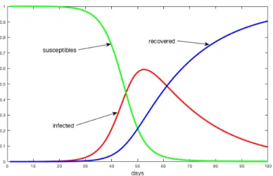
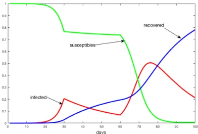
The classical SIR model in epidemiology
Tam metin
Şekil
Benzer Belgeler
Ders yazılım paketlerinin niteliğinin giderek artmasına paralel olarak matematik, fen bilimleri ve yabancı dillerin öğretiminde de bilgisayarların kullanımı
Mustafa İzzet Efendi'nin çocuk ları: Mehmet Efendi, Cemile Dür- riye Hanım, Mehmet Rıfat Bey, Ah met Necip Paşa, Abdullah Raşit E- fendi, Mehmet Ferit
闊別二十餘載 廿一屆同學會相見歡 (編輯部整理) 北醫廿一屆校友同學會於 101 大樓欣葉餐廳舉行,場面溫馨。
《遠見雜誌》首次完成「臺灣最佳大學排行榜」,北醫大獲私校第 1 《遠見雜誌》於 2016 年 9 月 29
N.: Immunocytochemi- cal Study of the Glial Fibrillary Addic Protein in Human Neoplasms of the Central Nervous System. W.W.: An Im- munohistochemical Study of Human Central and
Daha soma intraarteriyal (ia) veya intravenoz (iv) yolla verilen kontrast madde somasl goriintiiler elde edilir (~ekil : I-B).iki goriintii arasm- daki fark ahmr ki bu da
Gönen 2015 yılında Akdeniz Üniversitesi Beden Eğitimi ve Spor Yüksekokulu Öğrencilerinin İletişim Beceri Düzeyleri İle Atılganlık Düzeylerinin İncelenmesi
[r]
