Cash flow-at-risk in publicly traded non-financial firms in Turkey : an application in defense companies

CASH FLOW-AT-RISK IN PUBLICLY TRADED NON-FINANCIAL FIRMS IN TURKEY: AN APPLICATION IN DEFENSE COMPANIES

The Institute of Economics and Social Sciences

of

Bilkent University

by

Özhan ÖZVURAL

In Partial Fulfillment of the Requirements for the Degree of

MASTER OF BUSINESS ADMINISTRATION

in

THE DEPARTMENT OF MANAGEMENT BİLKENT UNIVERSITY

ANKARA

I certify that I have read this thesis and have found that it is fully adequate, in scope and in quality, as a thesis for the degree of Master of Business Administration.

---Prof. Kürşat AYDOĞAN Supervisor

I certify that I have read this thesis and have found that it is fully adequate, in scope and in quality, as a thesis for the degree of Master of Business Administration.

---Assoc.Prof. Faruk SELÇUK Examining Committee Member

I certify that I have read this thesis and have found that it is fully adequate, in scope and in quality, as a thesis for the degree of Master of Business Administration.

---Assist.Prof. Aslıhan SALİH Examining Committee Member

Approval of the Institute of Economics and Social Sciences.

---Prof. Kürşat AYDOĞAN

ABSTRACT

CASH FLOW-AT-RISK IN PUBLICLY TRADED NON-FINANCIAL FIRMS IN TURKEY: AN APPLICATION IN DEFENSE COMPANIES

ÖZVURAL, Özhan

M.B.A., Department of Management Supervisor: Prof. Kürşat AYDOĞAN

July 2004

People have always evaluated qualitative factors as black boxes so far. Academicians have put much effort to understand and explain these black boxes. The improvements in technology, therefore in social sciences, ease these efforts considerably. Risk is one of the qualitative factors, which drew people’s attention. As a result, some forecasting techniques have been developed to know the unknown. Risk means both profits and losses for people and firms. That is why, risk should be managed to exploit the profits and avoid the losses.

Value-at-risk relying on the data about liquid assets was proposed to assist financial firms such as banks, insurance companies, and investment companies to manage their risks. Contrary to financial firms, non-financial firms have more illiquid assets. These firms used value-at-risk to manage their risks initially but the practical results were not satisfactory. Therefore value-at-risk should be revised and adjusted to the non-financial firms. Consequently cash-flow-at-risk concept was proposed to manage risk in non-financial firms. This study aims to apply cash flow-at-risk concept in publicly traded non-financial firms in Turkey. The data drawn from financial statements were used because they helped to quantify risk in non-financial firms. The results of the study reveal that the proposed model can be used to asses all publicly traded non-financial firms’ risk exposure in Turkey for the next quarter.

ÖZET

TÜRKİYE’DEKİ HALKA AÇIK FİNANSAL OLMAYAN ŞİRKETLERDE RİSKE-MARUZ-NAKİT AKIMI :SAVUNMA ŞİRKETLERİNDE BİR

UYGULAMA

ÖZVURAL, Özhan

Yüksek Lisans Tezi, İşletme Bölümü Tez Yöneticisi: Prof. Kürşat AYDOĞAN

Temmuz 2004

İnsanlar kalitatif faktörleri bugüne kadar kara kutu olarak değerlendirmişlerdir. Akademisyenler kara kutu diye tabir edilen bu faktörleri anlamak ve açıklamak için büyük çaba harcamışlardır. Teknolojide ve de dolayısıyla sosyal bilimlerde yaşanan gelişmeler, bu çabaları büyük oranda kolaylaştırmıştır. İşte risk de insanların dikkatini çeken kalitatif faktörlerden birisidir. Bunun sonucu olarak, bilinmezliği öğrenmek maksadıyla bazı tahmin modelleri geliştirilmiştir. Şirketler içinde insanlar içinde risk kazançlar ya da kayıplar demektir. İşte bu sebepledir ki kazançlardan faydalanmak ve de kayıplardan kaçınmak için risk yönetilmelidir.

Riske-maruz-değer likit olan varlıklar hakkında bilgiye dayanıyor ve bankalar, sigorta şirketleri, ve yatırım şirketleri gibi finansal şirketlerde risk yönetimine yardımcı olmak maksadıyla ortaya atılmıştır. Finansal şirketlerin aksine, finansal olmayan şirketler daha fazla likit olmayan varlıklara sahiptirler. Bu şirketler, başlangıçta risk yönetimi maksadıyla riske-maruz-değeri kullanmış olsalar dahi uygulamaya dönük sonuçlar tatminkar olmamıştır. Bu yüzden, riske-maruz-değer finansal olmayan şirketlere göre yendien düzenlenmeli ve ayarlanmalıydı. Sonuç olarak, riske-maruz-nakit akımı finansal olmayan firmalarda risk yönetimi maksadıyla ortaya atılmıştır. Bu çalışma, riske-maruz-nakit akımı konseptinin Türkiye’deki halka açık finansal olmayan işletmelere uygulayı amaçlamıştır. Finansal tablolardan elde edilen bazı veriler finansal olmayan işletmelerde risk kavramını sayısallaştırmak maksadıyla kullanılmıştır. Çalışmanın sonucu , önerilen

modelin Tükiye’de bulunan tüm halka açık finansal olmayan şirketlerin bir sonraki çeyreğe ait maruz kalacakları riski değerlendirebilicağini göstermiştir.

Anahtar Kelimeler: Risk, riske-maruz-değer, riske-maruz-nakit akımı, finansal

ACKNOWLEDGEMENTS

I am very grateful to Prof. Kürşat AYDOĞAN for his supervision, constructive comments, and patience throughout the study. His vast knowledge and skill in finance added considerably to my M.B.A education. He became more of a mentor and respected senior than a professor. I also wish to express my thanks to Zeynep Özek VURAL for showing keen interest to the subject and accepting to read and review the thesis.

I would also like to thank my wife and daughter for the support they provided me throughout the study. I would not have finished this thesis without their love and encouragement.

TABLE OF CONTENTS

ABSTRACT…...……… iii

ÖZET……….. iv

ACKNOWLEDGEMENTS……… vi

TABLE OF CONTENTS……… vii

LIST OF TABLES……… ix

LIST OF FIGURES……… x

CHAPTER 1: INTRODUCTION……… 1

1.1 The Importance Of Risk Management……… 1

1.2 Capital Management, Risk And Shareholder Value…..……… 2

1.3 Definition Of The Problem………...…..……… 5

1.4 Scope Of The Thesis………...……… 8

CHAPTER 2. LITERATURE REVIEW…………...……… 10

2.1 Definition Of Risk……… 10

2.2 Value At Risk (VaR)………. 12

2.3 Cash Flow At Risk (C-FaR)………. 18

2.4 The Comparison Of Value At Risk With Cash Flow At Risk………… 25

CHAPTER 3. APPLICATION……… 27

3.3 General Framework……….. 27

3.3 Data Analysis….……… 34

3.3.1 Auto Regression Analysis………. 34

3.3.2 F Test……….…… 37

3.3.3 Distribution of Cash Flows……….. 38

3.4 Test….………. 43 3.4.1 Goodness-of-Fit Test………..… 43 3.5 Findings………...……….……… 45 CHAPTER 4. CONCLUSIONS………...……… 49 4.1 Conclusions………...……… 49 BIBLIOGRAPHY………...……….. 54 APPENDICES……….. 57

A. LIST OF NON-FINANCIAL FIRMS USED IN THE STUDY...……. 58

B. EBIT/TOTAL ASSETS OF THE FIRMS ………...…… 62

C. FORECAST ERRORS OF THE MODEL ………...………… 74

D. MARKET CAPITALIZATION AND STOCK PRICE VOLATILITIES OF FIRMS……….. 85

LIST OF TABLES

Table 1 Comparison of two C-Far models…...…….……… 22

Table 2 Summary statistics of EBIT/TA of 147 firms……… 33

Table 3 Some statistics of auto regression…...…….……… 35

Table 4 Summary statistics of bins…...…….……… 37

Table 5 Anderson-Darling statistics and p-values.……… 43

Table 6 Expected change in EBIT/TA values of the firms for the last quarter of 2003…...…….……… 48

LIST OF FIGURES

Figure 1 EBIT/Asset values of 147 firms….……… 32

Figure 2 EBIT/Asset values of 136 firms…….……….……… 34

Figure 3 Histogram of Bin-1…….……… 39

Figure 4 Histogram of Bin-2………. 39

Figure 5 Histogram of Bin-3…….……… 40

Figure 6 Histogram of Bin-4…….……… 40

Figure 7 Histogram of Bin-5…….……….. 40

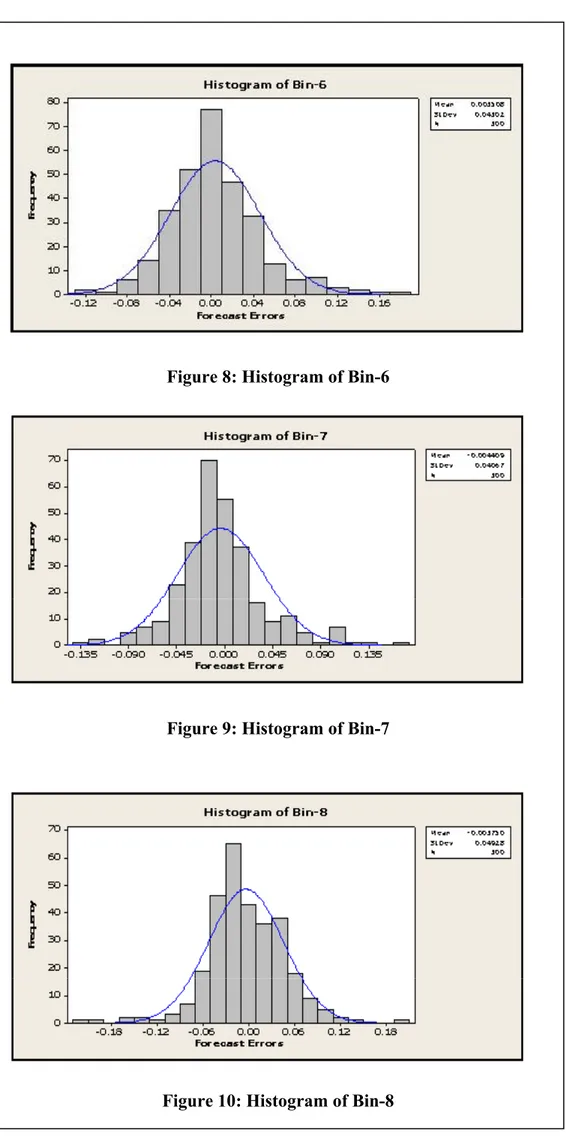
Figure 8 Histogram of Bin-6…….……… 41

Figure 9 Histogram of Bin-7……….……….. 41

Figure 10 Histogram of Bin-8…….……… 41

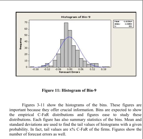
Figure 11 Histogram of Bin-9…….………. 42

Figure 12 Goodness-of-fit Test of Bin-1………..……… 44

CHAPTER I

INTRODUCTION

This chapter provides information about the importance of risk and its management. Then it explains the risk in non-financial organizations. The quantification of risk in non-financial firms, which is the basic idea of the thesis, is given in the problem definition section. The chapter concludes with the scope of the thesis.

1.1 The Importance Of Risk Management:

What will be the US dollar currency at the end of 2004 in Turkey? And what will be the €/$ parity? These are the common questions many Turkish company officials ask themselves. Turkish Central Bank (CB) started to implement floating exchange rates in February 2001. It became very difficult to forecast the exchange rates in Turkey since then. Exchange rates are important not only for financial firms but also for non-financial firms, especially if they are import or export based. Floating exchange rates increased the uncertainty for these firms. Uncertainty is by no means a synonym of risk for them because it is a major source of risk affecting

their survival. What about the other sources of risk? What are their effects to the firms? And finally what is the total risk the firms are exposed to?

Firms are operating in an ever-changing environment today. It is nothing but the change that affects every process in these firms. These changes show themselves as “globalization, disintermediation, innovation, and changes in regulatory environment, technological advancement and change in competitive structure of financial sector.” (Carlton, 1999) These changes have joint impact on firms’ risk exposure. These sources lead strategic, financial, operational, commercial, and technical risks for the firms. (Pricewaterhouse Coopers, 1997) These risk components’ joint impact on firms’ cash flow is regarded as the total risk of the firms. As a consequence, risk should be managed in firms for their survival.

1.2 Capital Management, Risk And Shareholder Value:

The academicians have thought risk as a variance of the expected returns. They suggest investors to minimize their portfolios’ variances in order to decrease their risk exposures. Is it the same for non-financial firms? How does risk management add value to shareholders in non-financial firms?

Firms having tradable, financial and mostly liquid assets such as banks, insurance companies, pension funds, securities firms and investment companies are regarded as financial firms. Whereas, production or service based firms having mostly illiquid assets are regarded as non-financial firms.

Risk management is indispensable component of a firm’s capital structure and strategic planning decisions. The right combination of risk management, capital structure and strategic planning is needed to optimize shareholder value. (Guth, 1996) The important problem is how to find this combination?

Risk management does not demand variance minimization in the non-financial firms’ cash flow. On the contrary, it demands just eliminating the downside risk of firms’ cash flow. Non-financial firms try to reduce the expected cost of financial trouble while preserving firms’ ability to utilize any comparative advantage in risk bearing. (Stulz, 1996) Non-financial firms direct their risk management towards shortfalls of the cash flow but not towards cash flow volatility as traditionally expected. Risk management in non-financial firms can constitute shareholder value if they focus on eliminating lower tail situations.

Modigliani and Miller (1958) proposed that the financial strategies do not add value under certain assumptions. They supported their propositions under a circumstance that there are no taxes, no costs of bankruptcy while operating cash flows are given and management acts to increase shareholder value. The risk management can add value from three perspectives if these assumptions are relaxed. These perspectives are:

• Risk management can reduce bankruptcy cost

• It can reduce payments to stakeholders and required returns to owners of closely held firms

Risk management can reduce bankruptcy cost just by decreasing the probability of financial distress. It is decreasing the direct and also the indirect costs. It is in fact decreasing the variability in the companies’ cash flows. When there is a risk for default, firms need more external funds than before. It is very apparent that financially weak firms face difficulties when raising funds. And these funds cost more to problematic firms if the funds are reachable. Reaching outside funds become so costly that these firms might lose to exploit profitable investments. Risk management can reduce the likelihood of such under-investment problems. (Froot et al. 1993)

Both private or closely held firms’ owners and stakeholders in public firms are anxious about the inability to diversify probable large financial exposures. These people heavily rely on the firms. That is, their considerable amount of investment is the shares they have in these firms. For that reason, risk management can add value by limiting uncontrolled financial exposures. Moreover, stakeholders from customers and suppliers to employees are always dubious about their self-interest. Customers expect the firms to fulfill their obligations. Suppliers, on the other hand, are reluctant to establish long-term relations with the problematic firms. As for the employees, they want to feel secure about the future of themselves. Risk management can ease potential tensions of the stakeholders.

Risk management is important because it can decrease the variability of the firms’ reported income. As in the U.S, it is very common that firms’ tax rates are proportional to their pre-tax income. Risk management seeks to minimize the tax and utilizes the tax-loss carry forwards of the firms’. The aim of these efforts is to keep

firms’ tax rate in an optimal range. That is why risk management plays a critical role in taxation.

1.3 Definition Of The Problem:

There are various risk components for non-financial firms, which jointly affect the firms’ cash flow stream. The firms’ total risk exposure must be managed in order to minimize this effect. Minimization of risk effects is important for the survival of these firms. And they are working hard to eliminate these effects they faced. They allocate remarkable resources on risk management by using information, technology, time and wisdom. As a result, they are still developing some basic tools. These tools are:

• Identification/Assessment tools, such as risk matrixes, which help firms’ management to identify and assess the risks exposing the firms.

• Categorization tools, which help management to group and prioritize, risk components. These tools are helpful because of using holistic view towards all risk factors.

• Financial quantification tools, such as cash flow-at-risk (C-FaR) model, which help firms to assess overall impact of risk factors in numbers. (KPMG, 2001)

C-FaR model is analogous to value at risk (VaR) model. One should know VaR model in order to be familiar with C-FaR. VaR is used commonly by financial firms to explore the effects of operating risks exposed by the firms. It also explores the potential effects of these risks on firms’ earnings. C-FaR can be interpreted as a

form of VaR for measuring total risk against non-financial firms’ cash flow. This analytic model helps non-financial firms to determine the probability of severe shocks to their cash flows and find their capital adequacy. (Wengroff, 2001)

In fact, C-FaR model helps non-financial firms to simulate the future to some extent. Non-financial firms can use this model to shape their strategic processes. The model is used explicitly to forecast the probable deviations in the earnings of the firms. It is assumed that firms’ total risk exposure, referred as a shock, directly affects their operating cash flows. The model helps the management of the firms to make their strategic decisions through the forecast. Moreover, quantification of cash flow volatility helps firms to comprehend downside and worst-case scenarios together with developing strategies to increase shareholder value under alternative business environments. Defense companies are among the probable non-financial firms having this idea in mind. They make significant investments, develop products, and take reasonable risks with respect to providing products and services to the security mission. These companies are in a rapidly changing technological environment and stiff competence. They must allocate considerable resources to R&D projects to survive but there is no guarantee to pay back their investments. That is why defense industry is seen one of the risky industries. C-FaR application in defense industry is expected to constitute good example for this respect.

Aselsan, Otokar and Netaş are three publicly traded defense firms in Turkey. The thesis intends to investigate the application of C-FaR model in these firms, in Turkish Army, and its participations, and in Turkey. This application is expected to guide other applications in non-financial firms as well. It will be easier to apply the

model in all publicly traded non-financial firms by the principles given in the thesis. C-FaR application in other non-financial firms, which are not publicly traded, will be also possible by making some changes in the model. C-FaR model is applied to three defense firms because they are concerned with managing the risks inherent in their operating cash flows like any other non-financial firms. The analytic model will help these firms to forecast their expected earnings and probable deviations in these earnings for the next quarter. These firms will also benefit from finding the effects of volatility in interest and exchange rates on firms’ cash flows. Following questions will be asked and expectantly answered in that sense:

• How much can defense companies and other non-financial firms’ operating cash flows be expected to decline in the last quarter of 2003? • Is the proposed model powerful enough to explain the answers of the

following questions?

• What are advantages and disadvantages of the model? • What are the test results of the model?

Information about sample firms is complementary tool for practitioners. That is why following sentences give basic information about the sample firms. The Turkish Armed Forces Foundation founded Aselsan in 20 November 1975. Objective of the firm is to produce tactical military radios and defense electronic systems for the Turkish Army. It is the leading multi-product electronics company of Turkey that designs, develops and manufactures modern electronic systems for military and professional customers. Nortel Networks Netaş is representative of Nortel Networks in Turkey. It provides networking and communication services and infrastructure to service providers, enterprises and Turkish Armed Forces in Turkey. Otokar, another defense firm, was founded to produce intercity buses in 1963 but it concentrated on

armor technology since mid-1980. It started to manufacture 4x4 tactical vehicles under license from Land Rover-UK in 1987. Today it manufactures armored Tactical Vehicles for military purposes in addition to its minibuses production. A sample application of C-FaR model in these defense firms is expected to be useful to understand the basics of the model and its application.

1.4 Scope Of The Thesis:

In the beginning, the importance of the risk was explained. The relation between risk, shareholder value and capital management fostered the necessity of its management. Risk perception in non-financial firms was also pointed. C-FaR, an analytical model was proposed to assist these firms to quantify their risk and make decisions for the future. Finally, the necessity to investigate C-FaR model was explained.

In the second chapter including literature review, detailed information will be given to understand the basics of risk concept. Why operating cash flow was selected to measure risk will be proved. In order to understand C-FaR model, both VaR and C-FaR concepts will be compared. Finally, the differences and similarities of two models will be discussed.

In chapter three, the data collection and EBIT/Total Assets notion will be interpreted. How the collected data was processed and model-building phases will be covered. The tests, which were done to check the power of the model, are presented

before the findings. As a consequence of the study, the findings will be discussed at the end of the chapter.

In the final chapter, summary and concluding remarks are presented. Avenues for future research are also discussed.

CHAPTER II

LITERATURE REVIEW

In this chapter C-FaR concept is defined by reviewing the literature on the sources of risk, risk management, VaR and C-FaR.

2.1 Definition Of Risk:

It is obvious that there have been many definitions of risk over years. The literature on risk is comprehensive. Origin of the word risk can be traced back to Latin, through the French “risqué” and the Italian “risco”. Risk concept is firstly seen in ancient Italian maritime trade. It was defined as the combination of chance or uncertainty to mean the loss of ships and cargo on the seas. Merchants used a term risk because of uncertainty they faced. (Jorion, 2001)

In a broader manner Hargreaves and Mikes (2001) defined risk as “Uncertain future events that could expose the firms to the chance of loss. Here, loss is a relative concept. It needs a reference level to be defined. The reference level is the list of the objectives stated in the business plan of the firms. Consequently, risk can be defined

as uncertain events that could influence the achievement of the firms’ strategic, operational and financial objectives.” Jorion (2001) further used risk as the volatility of unexpected outcomes, generally the value of assets or liabilities of interest.

It is very certain that risk components have considerable effect on the management of the firms, which should be examined carefully. Firms should manage risk because it offers both profits and losses. This management is entitled such as risk management or enterprise wide risk management. Briefly it is defined as a “process by which various risk exposures are identified, measured, and controlled.” (Jorion,

2001) Non-financial firms seek to benefit from their risk exposure while avoiding its catastrophic outcomes. There are many financial derivatives in financial markets to hedge the risks of the firms. These instruments help firms to manage their risks by using the tradeoff between risk taking and its rewards. Risk management has been one of the interesting topics for both academicians and practitioners. Although risk management is popular, there have been long debates about whether it can contribute to shareholder value or not. Debates are due to the complexity of risk concept and its management. It is complex because non-financial firms have difficulties to determine what type of risk to study. They haven’t decided what type of risk play considerable role in the survival of them.

Firms having high risk exposure, rely more on the cash flow than the others. Financial distress is main reason for this proposal. Facing high risk signals the financial weakness of the firms. Once they are financially weak today it is very probable that they are weak in the future. These firms need more external funds to survive. They need these funds to sustain their obligations. But it is not very easy for

these firms to find the needed funds because of having financing premium. Firms should carry the burden of higher costs of external funding than before. These firms are also in the risk of loosing chances of profitable investments. As a consequence, these firms are more cash-flow dependent. (Sterken et al. 2002)

All of the interpretations stated above underline the difficulty and the importance of risk and its management. Risk measurement and evaluation is hard work because risk is a qualitative element. How can non-financial firms estimate their over all risk? How can they evaluate their risk exposure? There is no problem if these firms’ incomes are more than their expenditures. But what if their expenditures are more than their incomes? They will soon go bankruptcy because of their inability to manage their risk.

Non-financial firms are in need of a quantitative tool to forecast their operating cash flows. Cash flow-at-risk, an analytic model was designed to help non-financial firms for that purpose. The model was developed from the roots of another analytic model Value-at-risk. In order to understand the usefulness of C-FaR, VaR model should be examined before hand.

2.2 Value At Risk (VaR):

“VaR is defined as a measure of the maximum potential change in value of a portfolio of financial instruments with a given probability over a pre-set horizon. VaR answers how much can the firm lose with x% probability over a given time

horizon.” (J.P Morgan/Reuters, 1996) Actors taking part in financial markets face risks such as counterparty default and market risk. Financial analysts use VaR as a measure to quantify market risk, which is the potential loss related with market behavior. VaR output, which is a single, summary statistical measure, stems from normal market movements. Greater losses than VaR expected have only small probabilities. The concept of VaR was emerged because of the significant efforts to measure market risk by academicians, practitioners and regulatory bodies. A statistical approach, VaR, and scenario analysis approach, revaluation of a portfolio under different values of market rates and prices, were two important outputs of these efforts. But what was the reason behind the increased interest about market risk measurement? The answer lies in the root of early studies about VaR and considerable changes that financial markets have experienced over years.

Leavens (1945) can be regarded as the pioneer of early VaR studies by his simple quantitative example. Although there were some scientists who covered the virtues of the diversification, Leavens, published his studies in a paper in 1945, which was the first, and the most comprehensive study about the benefits of diversification. Although he did not unequivocally present VaR model, he presented the spread between probable losses and gains for non-technical audience with the portfolio theory in his mind. (Leavens, 1945) Markowitz (1952) and later Roy (1952) followed Leavens by publishing the same VaR measures independently. The technology was not competent to prove the practical use of their findings in 1950s but their proposed measures were to support the portfolio optimization. They both presented the covariance between risk components for hedging and diversification

effects. Markowitz (1959) further published a book about his optimization scheme for computations.

William Sharpe (1963) used a better VaR measure in his Ph.D. thesis. Although the measure is different from Markowitz’s diagonal covariance matrix, it helped Sharpe to propose capital asset pricing model (CAPM). There were innovations in 1970s and 1980s in the financial markets as well as in every field of human life. The effect of these innovations was the rising of leverage. As this was the case, firms had a tendency to find new ways to manage risk. This in turn leads new measures of risk.

Garbade(1986) proposed VaR measures to model every bond upon its price sensitivity due to changes in yield. His model assumed that portfolio market values are normally distributed. The standard deviation of portfolio value can be found by the covariance matrix for yields at various maturities. His work drew little attention because Garbade was working for a private firm and his work was distributed only to clients. He further progressed his work in 1987.

Group of 30, a non-profit organization asked JP Morgan to lead a study of derivatives in 1992. Dennis Weatherstone, chairman of JP Morgan, formed a committee for that purpose. The committee’s final product was 68-page report published in July 1993. The report was published under the name of “ Derivatives: Practices and Principles” This document is significant because of being the first to use the word “value-at-risk” In October 1994 Guldiman from JP Morgan proposed a new system called RiskMetrics. It was a free computer system, which provides risk

measures for 400 financial instruments across 14 countries. These risk measures are forecasts of risk and correlations revised daily. The company pursued a noticeable public relation campaign to attract potential customers. (Holton, 2002)

In 1996 JP Morgan agreed with Reuters to cooperate on Risk Metrics. VaR notion was progressed and republished in a technical document in 1996. By the introduction of new RiskMetrics, managers can scale the data for their individual trading profiles. RiskMetrics provides covariance matrices to run VaR calculations. It also supplies the data for historical simulation and stress testing.

Financial markets were facing drastic changes by the rapid improvement in technology while the studies were going on about VaR between 1970s and 1990s. The management techniques were reshaping as the data processing was developing. New environment in financial markets was different because increased liquidity and pricing availability could ease the implementation of frequent assessment of positions, the mark-to-market concept. Firms became more interested in managing their daily earnings from a mark-to-market perspective. They were also interested in estimating the potential effect of changes in market conditions on their positions because of the slow but gradual increases in the volatility of earnings. Estimations in risk/return profile drew attention as well. Financial firms integrated their risk measurement process into their overall philosophy. They also formed and used market risk monitoring systems, which can provide timely information about positions and potential losses. All in all, these changes were about either performance or securitization. (J.P Morgan/Reuters, 1996)

Practitioners welcome the simplicity of VaR process because the basics of the VaR are very straightforward. It is also appealing because it offers market risk in a single number given the probability. (Manganelli, Engle, 2001) The management can use this number in boardroom, reporting to regulators and in firm’s annul reports for risk reporting, risk in internal capital allocation and performance measurement.

Beyond its benefits, managers do not solely trust VaR for their risk management. That is, VaR is an important tool in risk management but not unique. It is mostly used as a starting point because VaR is not sufficient in measuring event or market crash risk. Therefore managers sometimes go into detail and make more complicated analysis such as simulations and stress test. Greek letters such as delta, gamma and vega are in use as assistant tools as well. (Linsmeier, Pearson, 1996) In fact, it was designed by its creators to be used in derivative markets but it is now widely used by financial firms to measure their financial risks.

As for the full VaR models’ computation, there are three common approaches: Historical simulation, Monte Carlo simulation and parametric or variance-covariance approach. Historical approach is easy to use and demands few assumptions. It is mostly functional under a full valuation model. The profit and losses distribution of a portfolio is built upon current portfolio and subjecting it to actual changes during each of the last K periods, mostly days for financial firms. The computation of the theoretical profits and losses by actual historical changes in rates and prices is the distinctive feature of historical simulation. When the theoretical mark-to-market profit or loss for each of the last K periods have been calculated, the distribution of profits and losses and the value at risk, can then be found out.

The Monte Carlo simulation is not very different from historical simulation approach. The basic difference is about doing the simulation. Different from historical simulation approach, Monte Carlo simulation approach uses statistical distribution and artificial random generator to generate many theoretical changes in market factors. Then, these random numbers are used to build many portfolio profits and losses on the current portfolio and the distribution. Final step is to find value-at-risk from this simulated distribution. At the end, one can deduce that this method can facilitate in generating more paths of market returns than historical simulation.

Analytic method, used as an analogous for variance and covariance approach, is constructed upon market factors’ having multivariate normal distribution. It becomes possible with this assumption to find the distribution of mark-to-market portfolio profits and losses, expectantly normal. Basic mathematical calculations should be applied to find the loss by the help of normal distribution properties. Risk mapping, mapping actual instruments into a set of simpler and standardized positions, is the heart of this method. (Linsmeier, Pearson, 1996)

Implied volatilities and user-defined scenarios are two ways of calculations for the partial VaR models. Implied volatility is the market’s forecast of possible volatility in the future. It is mostly pull out from a particular option-pricing model to make comparison to history to distill risk analysis. Besides, user-defined rate and price movements are used as a complementary in case of historical patterns do not repeat themselves.

This section summarized the basics of VaR but remained one critical question, selecting appropriate measurement method. Each method shows

differences in capturing the risks of options, easiness in implementation, explanation, and reliability of results. The selection process is all apt to managers because cost and benefit trade-offs are different for each manager, his position in the market, the number and types of instruments traded and available technology.

2.3 Cash Flow At Risk (C-FaR):

C-FaR is defined as an analytic method of measuring with high degree of probability the risk of cash flow shocks for non-financial firms by its producers. This model helps firms by being a measure to evaluate the changes in their values. The model is proposed as a form of VaR for finding the overall risk against a firm’s cash flow. (Financial engineering news, 2001) C-FaR model tries to figure out the probability having inadequate cash to fund firms’ strategic investments. It is also defined as the “probability distribution of a firm’s operating cash flows over some time horizon in the future, usually the coming quarter or year, based on the information today.” These forward-looking probability distributions as in the VaR model are used to reach some statistics such as worst-case scenarios outcomes. These outcomes can be used by the management of the firms to measure the probability of rare negative events. It is evident that these negative events can produce a significant drop in the firms’ earnings. Furthermore, the model covers every source of potential risks, which firms can be exposed.

Since the more volatile a firms’ cash flow, the less debt it can safely carry in finance, the attention should be on the cash flow volatility of non-financial firms.

There are also three basic reasons to explain the importance of cash flow volatility. They are:

• Capital Structure Policy

• Evaluating hedging instruments and insurance strategies • Forecasting the earnings of the firms

The firms want to know their C-FaR for the purpose of their capital structure policy. Capital structure policy means the debt-equity choice of the firms. These firms try to exploit the benefits of debt against the potential costs such as financial distress. C-FaR helps firms to evaluate their probability of financial distress by interpreting the cash flow volatility. And C-FaR helps them to consider new investments and make strategic decisions.

Risk management and shareholder value correlation was discussed in the first chapter. In order to quantify the potential benefits of the risk management, non-financial firms need to have a holistic picture of their cash flow distributions. Firms can evaluate existing hedging instruments and insurance strategies by the help of this model.

Both institutional and individual investors are watching the earnings of the firms. This in turn, forces firms’ managements to achieve their planned goals. And investors can use C-FaR model to compare the expected earnings of the firms they are interested. The management of the firms’ can use it for the same purpose as well.

After the VaR model became popular, there were some expectations from risk consultants about VaR’s application in non-financial firms. VaR is very

applicable for financial firms but they are very different from the non-financial firms. Quantification of risk components and adding them up is easy for very liquid assets. Moreover, the data for liquid assets can be wide and easily reachable. This is not the same in non-financial firms, which have mostly illiquid assets. Potential problems would be solved if the overall thinking of VaR model were redesigned for non-financial firms.

Both academicians and practitioners worked together to progress new solutions as it is seen in the VaR case. Some consulting firms motivated academicians to apply VaR model to non-financial firms. These major firms are cited as RiskMetrics Group, which initiated the VaR model, Risk Capital Management Partners, and National Economic Research Associates (NERA). These companies compete with each other to produce the new product to non-financial firms. RiskMetrics was the winner of course. The company published a technical document in April 1999 by Alvin Y. Lee. The company proposed a new software package, CorporateMetrics, in this technical document. It is defined as a “conceptual framework for measuring market risk in the corporate environment.” (Lee, 1999) The

model quantifies the impact of market risks on earnings and cash flow. It shows the connection between changes in market rates and their effect on financial outcomes. There are basically five benefits for non-financial firms to use this model. These are increased transparency of risks, communicational benefits, hedging decisions, capital allocation and performance evaluation, and control. While these are the events for RiskMetrics other companies work hard to introduce their products.

In the mid 1999 National Economic Research Associates (NERA) vice president Stephen Usher formed a distinguished group of people. Nera is an international economic consulting firm who operates all over the world. Jeremy C. Stein from Harvard University economics department and two senior consultants Daniel LaGattuta and Jeff Youngen from NERA were the group members under the management of Stephen Usher. (Rich, 2001) Louis Guth senior advisor in Nera, Ken Froot and Paul Hinton supported the study. Omar Choudry and Amy Shiner were the research assistances of the team. (Stein, Usher, LaGattuta, Youngen, 2001)

The group was aiming to progress the VaR model application, especially to non-financial firms. The study group facilitates the new approach proposed by Hayt & Song’s (1995) study. Hayt & Song proposed a new bottom approach in their study. It associates the VaR. Contrary to Hayt & Song the study grouped used the top-down approach for C-FaR application.

Nera published the outcomes of the study in August 2000 by a working paper called “Comparables approach measuring cash flow at risk (C-FaR) for non-financial firms”. It was introduced as a computer-simulated method. The detailed findings were published in 2001 in the Journal of Applied Corporate Finance with the same title.

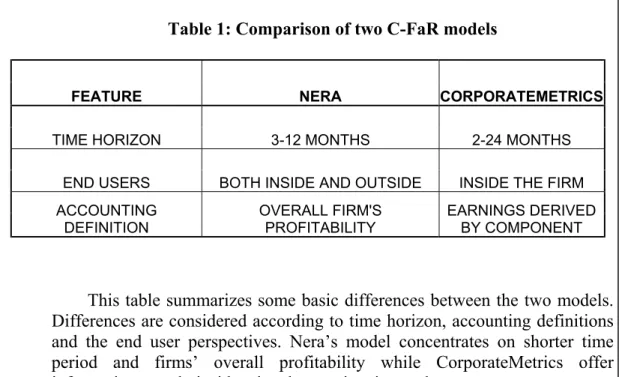
Table 1: Comparison of two C-FaR models

FEATURE NERA CORPORATEMETRICS

TIME HORIZON 3-12 MONTHS 2-24 MONTHS

END USERS BOTH INSIDE AND OUTSIDE INSIDE THE FIRM ACCOUNTING

DEFINITION OVERALL FIRM'SPROFITABILITY EARNINGS DERIVEDBY COMPONENT

This table summarizes some basic differences between the two models. Differences are considered according to time horizon, accounting definitions and the end user perspectives. Nera’s model concentrates on shorter time period and firms’ overall profitability while CorporateMetrics offer information to only insiders in a longer time interval.

The thesis intends to concentrate on the Nera’s C-FaR model and its application for practical purposes. Nera consultants aimed to obtain data on as many non-financial firms as possible. Then they used the quarterly income statement and the balance sheets of the firms. Four or five years’ quarterly data was seen enough for the application of the model. Earnings before interest and taxes, depreciation, and amortization (EBITDA) or earnings before interest and taxes (EBIT) was used as a basic measure for the operating cash flow. Firms’ EBITDA values were divided by the total assets of the firms, in order to compare them with each other. This scale, EBITDA/TA, was regarded similar to market-to-book, price to earnings or price-to-cash flow scale by the Nera committee. Then consultants smoothed the data by discarding the large scales, outliers. The outliers usually belonged to small firms. This smoothing was done for the elimination of having very large scales. Also scales having more than 50% changes in their assets were cleared. Consultants thought that

this move was for elimination of drastic changes in the firms’ assets. They also stated that change volume could be adjusted from 20%-to-%50 for practical purposes in the future studies.

Firms’ EBITDA/TA values would be used to forecast the expected cash flow. C-FaR model advocators needed a model to do this job and they used simple auto regression. EBITDA/TA scale in quarter t was regressed against four lags of itself. That is, EBITDA/TA in t-1, t-2, t-3 and t-4. t was the dependent variable and the other scales were the independent variables. The aim was not to make precise estimation but focusing on the entire probability distribution of shocks to cash flow, namely the tails of the distribution. The committee needed a benchmark for cash flows in the absence of shocks so that the forecast errors were used as deviations of cash flows from their expected values.

The data was collected only from recent six years for 3500 firms. Six-year data for these firms constituted 84000 forecast errors (6*4*3500=84000) for the U.S. As for a particular firm, six-year data meant 24 (6*4=24) forecast errors, which was not enough to make a judgment about cash flow volatility. On the other hand, pool of 84000 forecast errors contained different information about wide range of firms to the researchers. If firms and their errors were grouped according to similar characteristics then there would be small pools of forecast errors available for making inferences. Grouping meant dividing forecast errors into subsamples, which contain identical firms. Subsamples did contain neither 84000 errors nor 24 errors. They contained sufficient data to comment on firms’ cash flow volatility. Four characteristics were designated to divide forecast errors into subsamples. These were

market capitalization, profitability, industry risk and stock price volatility of the firms. Firms, which were in the same subsample, were expected to have similar cash flow volatility history as well. Similar firms were called peers, which have similar characteristics and background. That is why C-FaR is called as comparables based technique. Grouping was done through dividing the forecast errors into subsamples. The forecast errors were divided into three subsamples for firms’ market capitalization initially. Firms were compiled according to their market cap size. Top one-third of the firms and their forecast errors were regrouped in “market-cap bucket 1”, middle one third of them in “market-cap bucket 2” and the bottom one-third them in “market-cap bucket 3”. Each market-cap bucket was then divided into three subsamples according to second characteristic, namely profitability. After this process, there were nine forecast error buckets. The dividing process went on in this manner. Finally, there were 81 subsamples containing approximately more than 1000 forecast errors each. The researchers assumption was that forecast errors form an identical group of firms, peers. Each final subsample was regarded as “bin”.

In order to find any firms’ C-FaR, one should look at which bin it belongs to. The fifth percentile of the empirical distribution of the bin was regarded as the five-percent tail for a particular firm. Tail values of the bins were regarded as C-FaRvalues of the firms. And firm’s expected EBITDA would decrease as amount of tail intercept multiplied by the total assets in a five-percent worst-case. Briefly, the exact change in EBITDA is tail value times total assets. The outcome of the analysis was the final figure showing the change in operating cash flow of the firm in a five percent worst-case scenario. The probability was chosen as a five percent but can take other values as well. (Stein et al. 2001)

2.4 The Comparison Of Value-At-Risk With Cash Flow-At-Risk:

VaR model is called as a bottom-up method. That is, quantification of each risk component of the portfolio and adding them up. C-FaR method is referred as a “top-down” method on the other hand. Financial firms work mostly with liquid assets. Lets say a particular financial firm has a portfolio of three liquid assets. The VaR model’s bottom-up approach means finding risk exposure of its assets first and adding them up. The VaR model cannot be applied with the same approach to non-financial firms. If the bottom-up approach is used in non-non-financial firms, some significant risk elements are neglected. Therefore, it is very obvious to have misleading result if the bottom-up approach is used. In the top-down approach, the model looks at the assets overall risk exposure. The overall risk exposure can be found through the variations in firms’ operating cash flows.

Financial firms have high liquid assets. Their assets are easy to value but it is not the same for non-financial firms. Non-financial firms have assets, which are not easy to value because the assets cover both tangible and intangible components. Tangible assets are physical components such as property, plant and equipment. Intangible assets are brand, patent, and labor and supply agreements. It is very hard to value the assets of the non-financial firms because of this mixed structure.

VaR model also depends on normality assumptions. Contrary to VaR, C-FaR distributions appear to fatter-tailed than normal distributions, as well as somewhat right-skewed. VaR model demands more data than C-FaR. VaR model demands risk components’ historical data in a large scale. This is not applicable in the C-FaR

model because quarterly figures cannot be traced back more than five years. Although the data are available, the experts do not recommend it. Non-financial firms are rapidly changing and it is not healthy to go beyond this time frame.

CHAPTER 3

APPLICATION

The general framework section of this chapter is about the application of the C-FaR model. How the data were collected and analyzed was interpreted in this chapter. After the test of the model application, findings of the study are presented at the end of the chapter.

3.1.General Framework:

C-FaR is a model using current data by the comparables approach to draw conclusion. It is not an easy task to find the current data. Five-year period is a long-term strategic horizon for the firms. This period contains drastic volatility especially in an emerging market, like Turkey. This volatile climate limited us to choose five-year period data set for application because this volatility affects Turkish firms considerably from strategic planning to decision- making. Therefore it is very common to see that Turkish firms concentrate more on short term planning than their worldwide counterparts. Five-year period started from the fourth quarter of 1998 to the third quarter of 2003. The thesis intends to develop C-FaR model to quantify the

one-quarter ahead risk exposures of all non-financial firms in Turkey. Defense industry is not attractive for the investors because of high volatility. Therefore defense companies such as Aselsan, Otokar and Netaş will be good examples for the application of C-FaR model. The management can concentrate on only one figure to evaluate their total risk exposure.

The overall effect of risk components’ can be evaluated by the volatility of firms’ operating cash flow. Earnings before interest and tax (EBIT) was chosen to measure the operating cash flows. A forecasting model is needed to find forecast errors, that is, expected changes in the firms’ operating cash flows. Each firm will have 20 forecast errors for the five-year time period. These are not enough to comment on the firms’ cash flow volatility. Consequently, group of identical firms are needed because forecasting model depends on only one particular firm to estimate volatility in cash flows does not meet the expectations scientifically. Group of identical firms mean more forecast errors to facilitate making the decisions. The EBIT values, which are the indicators of the operating cash flows, are to be regressed against four lags of itself for the selected time period. These values are different for every firm. As a result, EBIT values were divided by the total assets. The forecast errors of the forecasting model are deviations in EBIT/TA. These forecast errors will be grouped according to two characteristics. These are market capitalization and stock price volatility. First forecast errors will be divided into three sub-samples according to market capitalization. Then each sub-sample will be divided into three sub-samples again according to stock price volatility. In the end, there will be nine sub-samples containing a sufficient number of forecast errors. The bucket of nine forecast errors will help in making decisions. That is, the histogram of the forecast

errors can be judged from different points. These histograms of forecast errors enable us to come up with a single number showing non-financial firms’ total risk exposure.

Advantages and disadvantages, power, and the test of the model were explored and the detailed findings were presented for future studies in this chapter as well. The details of the application will be presented in the following sections.

3.2 Data Collection:

Stock markets are not only economical actors but also reliable sources of information for public. They put the transparent, reliable and audited information about the firms into the use of investors. The Istanbul Stock Exchange (ISE) database was designated as a primary source of information for that reason. ISE offers not only the historical data about Turkish firms but it also revises firms’ financial statements in each quarter.

C-FaR model demands comparable or peer non-financial firms to comment on a particular firm. ISE offers financial information about major companies in Turkey. These companies belong to different industries. The first step in the data collection is to decide which industries should be chosen to evaluate non-financial firms. Therefore food and beverage, textile and leather, wood, paper and printing, chemical, petroleum and plastic, non-metal mineral product, basic metal, metal products and machinery, information technology, defense, second national industries were selected.

The five-year period was chosen to collect past data for the firms in the sample. Each firm has totally 20 quarterly data for the period under examination. The ISE was founded in 1986 with fewer firms than it has now. As time went by, it lures many other firms who were seeking capital. New firms were quoted to ISE year by year. There were 156 non-financial firms, which were publicly traded in ISE in 1998. The firms, in alphabetical order, are presented in Appendix A. Some firms in 156 are not traded in ISE today for several reasons. There are also some firms with incomplete data. That is, they were not traded for a particular time in 1998-2003. Therefore they were removed from the sample. The remaining 147 firms were all included in the sample. The quarterly financial data were obtained through their income statement and balance sheets.

Earnings before tax and interest (EBIT) is the basic measure for the operating cash flow of the non-financial firms. EBIT can be obtained from firms’ income statement. The profit before tax and financial expenses are the two components of the EBIT. Financial expenses figure should be added to profit before tax figure to find EBIT.

There is no problem to find the profit of the firms for each quarter. Income statements show the cumulative magnitude over the year. That is, second quarter’s profit includes both the profit in the first and second quarter. The first quarter’s profit should be deducted from the second quarter’s profit in order to find the second quarter’s net profit. This is the same for third and fourth quarter of the firms as well. The only net value of the firms’ profits can be attainable in the first quarters. When you look at the profit figure in the income statement of the first quarter, the figure

points the firms’ net profit for that quarter. The firms can have either profits or losses. Briefly, when looking at the profit before tax figure from income statement, attention should be concentrated on whether the firm profits or have losses. That is, the sign of the figure is very important.

In fact, there are some important problems when finding the financial expenses figure. This figure is in the income statement and behaved like the profit before tax figure. Financial expenses figure has normally a negative sign. When this figure is deducted from profit before tax, in fact it is added to profit before tax. Nevertheless, data collection process showed that there are some quarterly financial expenses figures, which have positive signs. That is, the firms have not financial expenses but rather gain in that period.

The situation can be explained by two factors: Foreign exchange rate volatility and volatility in cost of goods sold. The foreign exchange rates fluctuate due to the floating exchange rates policy of Turkish Central Bank (CB) in Turkey since February 2001. As a result of this policy, firms’ financial expenses show volatility. The designated currency in the previous quarters may drop against the TL in the later quarters. With this information in mind, some positive financial expenses figures were obtained for some quarters. These figures should be deducted from profit before tax figure. These figures were really deducted from profit before tax because they have positive sign. This is the same for the cost of goods. Firms, which have export or import relations, have difference in cost of goods because of foreign exchange fluctuations. The difference is sometimes reflected as positive financial expenses.

The EBIT figure shows differences for each firm. This figure is not sufficient to comment on operating cash flows. In order to overcome the scale differences problem between firms, EBIT is divided by total assets. The new scale can be used for the comparative purposes since then. The EBIT/TA scale can be regarded as analogous to market-to book, price to earnings or price-to-cash flow rates.

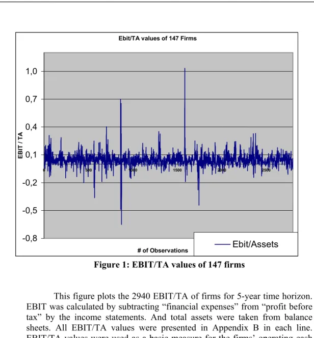
Figure 1: EBIT/TA values of 147 firms

This figure plots the 2940 EBIT/TA of firms for 5-year time horizon. EBIT was calculated by subtracting “financial expenses” from “profit before tax” by the income statements. And total assets were taken from balance sheets. All EBIT/TA values were presented in Appendix B in each line. EBIT/TA values were used as a basic measure for the firms’ operating cash flow.

Ebit/TA values of 147 Firms

-0,8 -0,5 -0,2 0,1 0,4 0,7 1,0 0 500 1000 1500 2000 2500 # of Observations EBIT / TA Ebit/Assets

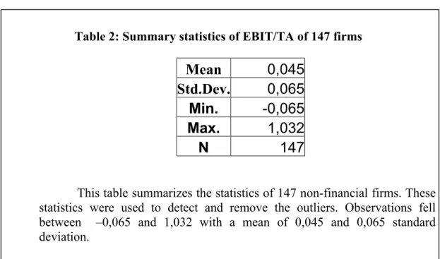
Table 2: Summary statistics of EBIT/TA of 147 firms

Mean

0,045

Std.Dev.

0,065

Min.

-0,065

Max.

1,032

N

147

This table summarizes the statistics of 147 non-financial firms. These statistics were used to detect and remove the outliers. Observations fell between –0,065 and 1,032 with a mean of 0,045 and 0,065 standard deviation.

According to empirical rule in statistics, approximately 99,7% of measurements falls within three standard deviations of the mean (µ - 3σ, µ + 3σ). (Mcclave et al. 2001) The 3,8 standard deviation was selected for this study. The number 3,8 standard deviation stems from the principles of the study. It is to find as many firms as possible. As a result of this process 136 of 147 firms found suitable to work on. That is, 92,52% of measurements were used. Eleven firms, Adel Kalemcilik, Brova Yapı, Çbs Boya, Dardanel, Feniş Aluminyum, FM İzmit Motor Piston, Işıklar Ambalaj, Kerevitaş Gıda, Kelebek Mobilya, Çbs Printaş Baskı, and Park Elektrik Madencilik were removed from the list. And these firms are the outliers.

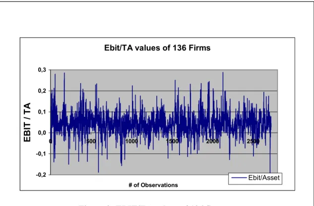
Figure 2: EBIT/TA values of 136 firms

This figure plots the 2720 EBIT/TA of 136 firms after eliminating the outliers. The values fell between –0,2 and 0,3. These observations contain 92,52% of all observations. This figure also shows the strength of the model because EBIT/TA values do not show extreme deviations on average.

3.3 Data Analysis:

3.3.1 Auto Regression Analysis:

The basic goal of the study is to find the deviations in cash flows of the firms in the sample. In order to do so, the forecast of the cash flows is needed. That is, there should be a model to forecast the next quarter’s cash flow. The simple multivariate regression analysis was used as a forecasting model. EBIT/TA t demonstrates the EBIT to total assets ratio in quarter t in the model. This was regressed against four lags of itself, which equates in auto regression in Microsoft Excel 2000. The result is given in the equation 3.1.

Ebit/TA values of 136 Firms

-0,2 -0,1 0,0 0,1 0,2 0,3 0 500 1000 1500 2000 2500 # of Observations EBIT / TA Ebit/Asset

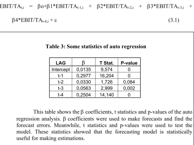
EBIT/TAt,i = βo+β1*EBIT/TAt-1,i + β2*EBIT/TAt-2,i + β3*EBIT/TAt-3,i +

β4*EBIT/TAt-4,i + ε (3.1)

Table 3: Some statistics of auto regression

This table shows the β coefficients, t statistics and p-values of the auto regression analysis. β coefficients were used to make forecasts and find the forecast errors. Meanwhile, t statistics and p-values were used to test the model. These statistics showed that the forecasting model is statistically useful for making estimations.

Other combinations were used to yield a better predictive power but they were not better than the combination used. The five-year quarterly data was used for each firm. In fact, the model needs more than five-year data. The quarterly data includes the fourth quarter of 1998 through the third quarter of 2003 with the total of 20 observations. Nevertheless, in order to regress the fourth quarter scale against four lag of itself, the data between the fourth quarter of 1997 and the third quarter of 1998 are needed. In fact, the model used six-year data.

Adjusted R square value is 0,24 which means that the model has explained about 23,99% of the total sample variation in EBIT/TA value, after adjusting for sample size and number of independent variables in the model. (Mcclave et al. 2001: 556)

LAG β T Stat. P-value

Intercept 0,0135 9,574 0 t-1 0,2977 16,204 0 t-2 0,0330 1,726 0,084 t-3 0,0563 2,999 0,002 t-4 0,2504 14,140 0

The shocks correspond to forecast errors in the model. Forecast errors are deviations from their expected value. 136 firms with 20 observations offer 2720 forecast errors to study. The forecast errors of the firms are presented in Appendix C. The group of forecast errors is very important in this study. They are regrouped according to two characteristics. One is market capitalization, and the other is stock price volatility. Appendix D shows the market capitalization of the firms at the end of the third quarter of 2003 together with the stock price volatilities. The stock price volatility is calculated by the variance of the firms’ monthly stock price returns from the fourth quarter of 1998 to the third quarter of 2003. Two characteristics were chosen for having little or no correlation. That is, 136 firms’ market capitalization correlation with stock price volatility is –0,099 with 0,252 p value. There is an expectation about being little correlation between two characteristics because model would be biased if they were correlated high.

The firms were grouped according to their market capitalization as a first step. The top one-third firms consist of “market-cap bucket 1”, the middle one-third firms consist of “market-cap bucket 2”, and the bottom-third firms consist of “market-cap bucket 3”. Then each market cap bucket is further grouped into three sub samples according to firms’ stock price volatility; that is, variance of their monthly stock price returns. Finally there were eight identical buckets having 15 firms and one final bucket of 16 firms. These forecast errors of the firms’ were placed into buckets, or bins, 2720 forecast errors are distributed into 9 bins according to how firms were grouped. Consequently, there are eight bins having 300 forecast errors and one bin having 320 forecast errors. The first bin, bin-1 shows the most risky firms with the highest market capitalization. The last bin, bin-9 shows the least

risky firms with the lowest market capitalization. Appendix D shows firms’ bin classification.

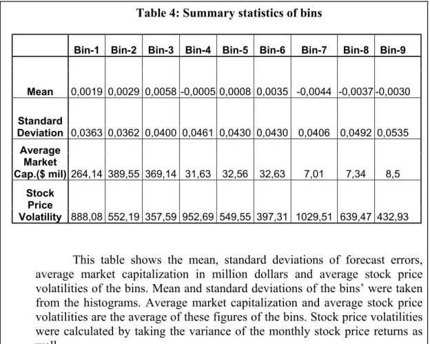
Table 4: Summary statistics of bins

Bin-1 Bin-2 Bin-3 Bin-4 Bin-5 Bin-6 Bin-7 Bin-8 Bin-9

Mean 0,0019 0,0029 0,0058 -0,0005 0,0008 0,0035 -0,0044 -0,0037 -0,0030 Standard Deviation 0,0363 0,0362 0,0400 0,0461 0,0430 0,0430 0,0406 0,0492 0,0535 Average Market Cap.($ mil) 264,14 389,55 369,14 31,63 32,56 32,63 7,01 7,34 8,5 Stock Price Volatility 888,08 552,19 357,59 952,69 549,55 397,31 1029,51 639,47 432,93

This table shows the mean, standard deviations of forecast errors, average market capitalization in million dollars and average stock price volatilities of the bins. Mean and standard deviations of the bins’ were taken from the histograms. Average market capitalization and average stock price volatilities are the average of these figures of the bins. Stock price volatilities were calculated by taking the variance of the monthly stock price returns as well.

3.3.2 F Test:

Adjusted R square is just a sample statistic in spite of its helpfulness. It is misleading to comment on the global usefulness of the model based only on adjusted R Square. Hypothesis involving all the β parameters should be tested with a better method. The hypotheses are as follows:

Ho: β1= β2 = β3 = β4 =0

Ha: at least one of the coefficients is nonzero

F statistics was used to test the hypotheses. F statistic is the ratio of the explained variability divided by the forecasting model degrees of freedom to the unexplained variability divided by the error degrees of freedom. The rejection region is:

F > Fα where F is based on 4 numerators and 2695 denominator degrees of freedom.

α was designated 0,05 for this study. Since it exceeds the observed significance level 9,1E-161 the data provide strong evidence at least one of the model coefficients is nonzero. As a result, the overall model used for cash flow estimation appears to be statistically useful for estimation. (McClave et al. 2001: 558)

3.3.3 Distributions of Cash Flows:

C-FaR model expects that the forecast errors come from a relatively homogenous group of firms, which were matched on the two characteristics. When this assumption holds true, there is a powerful parametric way to find the C-FaR of any given firm. The 300 forecast errors for each firm can well describe their C-FaR distribution. That is, C-FaR needs to analyze the forecast errors distribution of each bin. The histogram of the each bin can be used for this purpose. Minitab Release 14 for Windows program was used to get the histograms of the forecast errors in each

bin. The histograms of the forecast errors permits to evaluate any tail value for the empirical distribution.

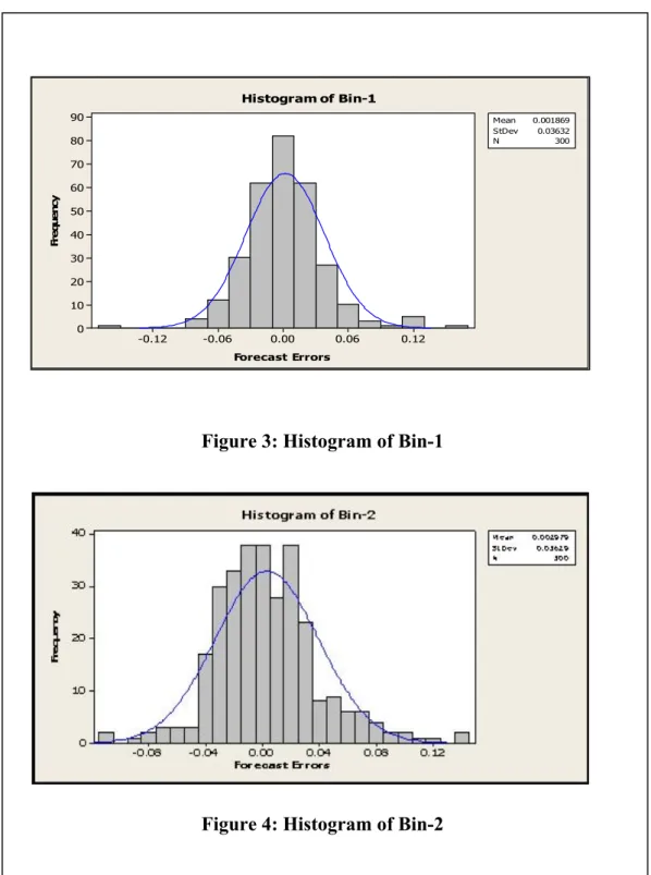
Figure 3: Histogram of Bin-1

Figure 3.4. Histogram of Bin-2

Figure 4: Histogram of Bin-2

Forecast Errors Fr e q ue nc y 0.12 0.06 0.00 -0.06 -0.12 90 80 70 60 50 40 30 20 10 0 Mean 0.001869 StDev 0.03632 N 300 Histogram of Bin-1

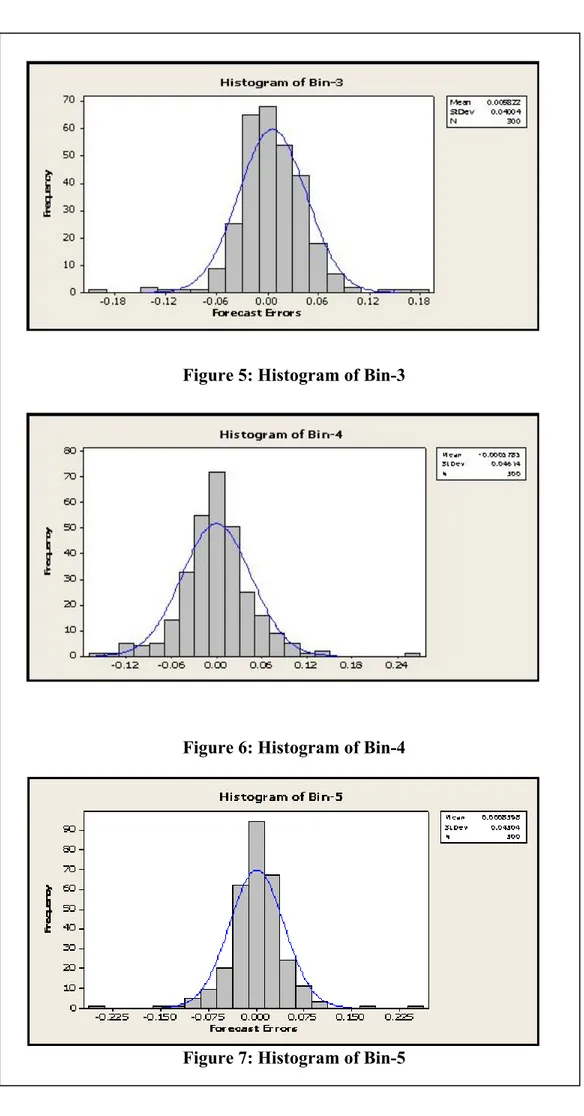
Figure 5: Histogram of Bin-3

Figure 6: Histogram of Bin-4

Figure 8: Histogram of Bin-6

Figure 9: Histogram of Bin-7

Figure 11: Histogram of Bin-9

Figures 3-11 show the histograms of the bins. These figures are important because they offer crucial information. Bins are expected to show the empirical C-FaR distributions and figures ease to study these distributions. Each figure has also summary statistics of the bins. Mean and standard deviations are used to find the tail values of histograms with a given probability. In fact, tail values are x% C-FaR of the firms. Figures show the number of forecast errors as well.

In order to find the exact C-FaR value of a particular company, which bin the firm belongs to should be clarified. Then the histogram of the designated bin should be analyzed by the given probability. Mean and the standard deviations of the distributions are needed for this analysis. The analysis is just the same as finding the tail values of any normal distribution by given probability.

3.4 Test:

3.4.1 Goodness-of-Fit Test:

Although C-FaR distributions appear to be fatter-tailed than normal distributions, a formal test of the normality was conducted. Normality test generates a normal probability plot and performs a hypothesis test to examine whether or not the observations follow a normal distribution. (D’Agostino, Stephens, 1986) Anderson-Darling statistic was used to determine if the data follow a normal distribution. If the p-value is lower than the pre-determined level of significance, the data do not follow a normal distribution. Smaller Anderson-Darling (AD) values indicate that the distribution fits the data better. The AD values were used to compare the fit of competing distributions as opposed to an absolute measure of how a particular distribution fits the data. For the test, the hypotheses are as follows:

Ho= Data follow a normal distribution Ha= Data do not follow a normal distribution

Table 5: Anderson-Darling statistics and their p-values of the bins

Bin-1 Bin-2 Bin-3 Bin-4 Bin-5 Bin-6 Bin-7 Bin-8 Bin-9

A.D 2.238 2.459 2.591 2.835 4.117 2.591 4.788 1.824 3.989

p-value <0.005 <0.005 <0.005 <0.005 <0.005 <0.005 <0.005 <0.005 <0.005

This table shows Anderson-Darling statistics and their p-values of the bins at the significance level of 5%. Anderson-Darling statistics and p-values were used to test the normality distribution of the bins. Since all the p values of nine bins are less than significance level 0,05 the null hypothesis was rejected for all bins. As a result, forecast errors of the non-financial firms, do not follow a normal distribution.

Appendix E shows the graph of the each bins’ normality distributions. Aselsan and Netaş belong to bin-1 and Otokar belongs to bin-4.

Figure 12:Goodness of fit test for the Bin-1

Figure 13:Goodness of fit test for the Bin-4

Figure 12-13 shows whether the forecast errors follow normal distribution or not. Statistics of the bins were interpreted in the figures as well. Values abbreviated in AD are Anderson-Darling statistics. p-values are used together with AD values to test the normality hypothesis. If p-values are less than significance level than the H o is rejected, meaning that data do not

follow normal distribution.

Pe rc e n t 0 .2 0 .1 0 .0 - 0 .1 - 0 .2 99 .9 99 95 90 80 70 60 50 40 30 20 10 5 1 0 .1 M e a n < 0.00 5 0 .0 01 86 9 S tD e v 0.03 63 2 N 30 0 A D 2.23 8 P - V a lu e P r o b a b i l i ty P l o t o f B i n -1

3.5 Findings:

Aselsan, Netaş and Otokar are three important publicly traded defense companies in Turkey. These companies were chosen to interpret the results of the model’s application. The deviations in these companies’ operating cash flows are presented successively in the following paragraphs with related calculations. The probability was chosen to be 5% for the study. In order to find any non-financial firms’ C-FaR value one should look at which bin does it belong to? The histograms of forecast errors of bins were presented in figures 3.3 to 3.11. Statistics in the graphs are used to make final decisions about operating cash flow deviations.

Aselsan belongs to first bin, which has a mean of 0.001869 and a standard deviation of 0.03632. Z value for the 5% probability is -1.645. The equation for the tail value is as follows:

(X - µ) /σ = z (3.2)

Where µ = 0,001869 σ = 0,03632 z = -1,645

The tail value (x) is equal to –0,05788. This number is multiplied by the total assets of Aselsan in the last quarter of the data set, namely the third quarter of the 2003. That is, TL 647.654.844.

-37.484.578TL is the expected loss in the EBIT of Aselsan. The percentage of the loss can even be calculated easily. The loss figure should be divided by the EBIT of the last quarter of the data set.

-37.484.578,47 / 34.742.869 = -1,07891 or 107,9%

Aselsan’s operating cash flow is expected to decline 37.484.578TL over the next quarter if the firm faces a downturn that turns out to be a five-percent tail. Finally, -2.741.709TL is the firm’s expected operating cash flow for the next quarter in case of a five-percent tail downturn.

Netaş belongs to the first bin as Aselsan does. Therefore the tail value for Netaş is identical with Aselsan, namely –0,05788. This number is multiplied by the total assets of Netaş in the third quarter of 2003, namely 191.150.357TL

191.150.357 * -0,05788 = -11.063.782,66

-11.063.783 is again the expected loss in the EBIT of Netaş. The percentage of the loss is:

-11.063.782,66 / 14.136.281 = -0,7827 or 78,3%

Netaş’s operating cash flow is expected to decline 11.063.783 over the next quarter if the firm faces a downturn that turns out to be a five-percent tail.