On Arf rings

; . 5«ÎJ4.5·

^ ·. » ¥'■»>,·· 0 ¡e* i w -«et -«jf

r n, Λ ·;'·■'

ON ARF RINGS

A THESIS

SUBMITTED TO THE DEPARTMENT OF MATHEMATICS AND THE INSTITUTE OF ENGINEERING AND SCIENCES

OF BILKENT UNIVERSITY

IN PARTIAL FULFILLMENT OF THE REQUIREMENTS FOR THE DEGREE OF

MASTER OF SCIENCE

By

Sefa Feza Arslan September, 1994

и й

6 4 S

-f-ИЯ-I certify that -f-ИЯ-I have read this thesis and that in my opinion it is fully adequate, in scope and in quality, as a thesis for the degree of Master of Science.

Asst. Prof. Dr. oinan Sertóz(Pnncipal Advisor)

I certify that I have read this thesis and that in my opinion it is fully adequate, in scope and in quality, as a thesis for the degree of Master of Science.

fp.is r

Assoc. Prof. Di

Assoc. Prof. Dr. Hursfit Onsiper

I certify that I have read this thesis and that in my opinion it is full}* adequate, in scope and in quality, cis a thesis for the degree of Master of Science.

Assoc. Prof. Dr. Varol Akman

Approved for the Institute of Engineering and Sciences:

Prof. Dr. Mehmet

ABSTRACT

ON ARF RINGS

Sefa Feza Arslan M .S . in Mathematics

Advisor: A sst. Prof. Dr. Sinan Sertöz September, 1994

In this thesis, we worked with curves which have cusp type singularities. We described the Arf theory, which solves the problem of understanding and finding the multiplicity sequence of a curve branch algebraically. We proposed an algorithm for finding the Arf characters of a given curve branch. We also faced the problem of Frobenius, and proposed an algorithm for the solution of problem of Frobenius in the most general case.

Keywords : Curve branch, singularity, blow up, multiplicity sequence, Arf ring, A rf semigroup, Arf closure, Arf characters, Frobenius.

ÖZET

A R F H A L K A L A R I

Sefa Feza Arslan

M atem atik Bölüm ü Yüksek Lisans Danışm an: A sst. Prof. Dr. Sinan Sertöz

Eylül, 1994

Bu tezde, köşe noktası biçiminde tekillikleri olan eğrilerle ilgilendik. Bir eğri kolunun çokkatlılık dizisinin anlaşılması ve bulunması sorununu cebirsel olarak çözen Arf kuramını tanıttık. Verilen bir eğri kolunun Arf karakterlerini bulan bir algoritma önerdik. Ayrıca, Frobenius problemi ile de karşılaştık ve en genel durumdaki çözümü için bir algoritma önerdik.

Anahtar Kelimeler : Eğri kolu, tekillik, tekilliğin çözülmesi, çokkatlılık dizisi, Arf halkası, Arf yarıgrubu, Arf kapanışı, Arf karakterleri, Frobenius.

ACKNOWLEDGMENTS

I would like to thank to Asst. Prof. Dr. Sinan Sertöz for his supervision, for his continued guidance, for his readiness to help at all times, for his critical comments while reading the written work, and for his encouragement through the development of this thesis.

I would like to thank Berna, who gave me hope with her love and support when I found myself in times of trouble.

I would also like to thank Göksen for his great help in computer graphics, and for his friendship.

I would like to thank my family for their love and support.

It is a pleasure to express my thanks to all my friends, with whom I shared everything; good times, bad times, agonies, hopes, and utopias.

TABLE OF CON TENTS

1 INTRODUCTION

1

2 CURVES, SINGULARITIES, AND RESOLUTION OF SIN­

GULARITIES

3

2.1 B a ck g rou n d ... 3

2.2

C u r v e s ... 12

2.3 Singularity... 16

2.4 Resolution of S in gu larities... 18

3 ARE CHARACTERS OF SINGULAR BRANCHES

23

3.1 Historical D evelopm ent... 23

3.2 Arf Rings, Closure and Characters 28

4 THE PROBLEM OF FROBENIUS AND AN ALGORITHM

FOR ITS SOLUTION

40

4.1 The Problem of F r o b e n iu s ... 40

4.2

An Algorithm for the Solution of the Problem of Frobenius . . . 43

5 AN ALGORITHM FOR FINDING THE ARF CHARAC­

TERS OF A BRANCH

47

6 CONCLUSION

7 APPENDIX

58

LIST OF FIGURES

2.1

Pr ...

11

2.2 The cuspidal cubic curve and the nodal cubic c u r v e ... 13

2.3 Four-leaved r o s e ... 14

2.4 The blow up X of 19

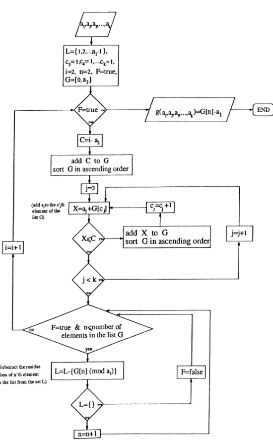
4.1 Flow chart of the Algorithm for the problem of Frobenius . . . . 46

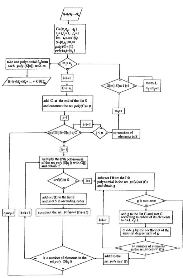
5.1 Flow chart of the Algorithm for the construction of / / ... 54

Chapter 1

INTRODUCTION

The link between algebra and geometry makes it possible to predict alge­ braically the result of a geometric process. In this way, a geometric problem can be solved by algebraic methods and computations. Also, invariants of a geometric object can be found algebraically; these are very important for classification.

We will deal with curves, which have cusp type singularities. Singular curves can be classified by finding nonsingular curves, which are birationally equivalent to these singular curves. This can be done by a blow up process. For cusp type singularities, one blow up may not be sufficient to remove the singularity. Hence, successive blow ups must be applied to obtain a nonsingular curve. The multiplicity sequence constructed by taking the multiplicity o f the singularity before each blow up is a fundamental invariant of the singularity. Arf shows that the completion of the local ring at the singularity of the branch carries all the information necessary to obtain the multiplicity sequence [

2

].

A rf passes from geometry to algebra by using the completion of the local ring. He constructs the canonical closure of this ring, later called the Arf closure. The orders of the elements of this ring form a sub-semigroup o f the natural numbers. In this way, Arf passes from algebra to arithmetic. From this semigroup, Arf obtains some numbers by a process to be described later, and then he determines the multiplicity sequence of the curve branch by applying the modified Jaccobian algorithm [

8

, pp. 108-109] to these numbers. These numbers are called the Arf characters of that curve branch.

The purpose of this thesis is to describe the work of Arf and to propose a computer algorithm for finding the Arf characters of a given curve branch.

Because of the the sub-semigroup mentioned above, we face the problem of finding the largest integer which is not included in this semigroup, if the gen­ erators of this semigroup are relatively prime. This is the famous problem of Frobcnius. We also propose an algorithm for the solution of the problem of Frobenius in the most general case.

In chapter

2

, we give the necessary preliminaries for understanding the Arf theory. We describe the category in which we will be working, by defining its objects and morphisms. Then we describe curves, singularities, and resolution of singularities, and give examples.

In chapter 3, we present a history of the problem of obtaining the multiplic­ ity sequence of a singular curve branch without applying succesive blow ups to the curve. Then we describe the work of Arf and his solution to this problem.

In chapter 4, we offer a literature review of the problem of Frobenius. This involves looking for the largest integer that is not included in the semigroup generated by relatively prime integers. Then we propose an algorithm for the solution of the problem of in the most general case.

In chapter 5, to find the Arf characters of a curve branch we propose an algorithm applicable to computer, by depending on the work of Arf. In this al­ gorithm, given a parameterization of a curve branch as input, its Arf characters are obtained as output.

We use the following notation throughout:

R = Real numbers

Chapter 2

CURVES, SINGULARITIES,

AND RESOLUTION OF

SINGULARITIES

2.1

Background

We will be working in the category of algebraic varieties and birational maps over an algebraically closed field. Our main construction is a blowing up of an algebraic variety, which is the main example of a birational map. We recall some definitions.

Let k be an algebraically closed field.

D efin ition

2

.

1

.

1

. An affine n-space over k is defined to be the set of all n-tuples, components of which are from k. An affine /i-space over k is denoted by A^, and by A ” if no confusion about the field arises.

It looks as if A " and k^ are the same but there is a major difference, k^

has an origin and a vector space structure, but A" is just a set of points. In the origin is a distinguished point, however in A" all points are considered with equal attention and no point is distinguished.

Let A = ...,T„] be the polynomial ring in n variables over k. If / is a polynomial in A and a = (<Ji,...,a„) is an element of the affine space A ", then

all a G A ” satisfying /( a ) =

0

.

If 5 is a collection of polynomials from A, then

Z(S) = {a

6

A" I /(a) =

0

for all /

6

Sj,

is the set of all simultaneous solutions of the polynomials in S.

If / is the ideal generated by S, then one can show that Z(S) — Z{I). It follows from Hilbert's basis theorem that A — /;[xi, ...,^»

1

] is a Noetherian ring. (See for example [3, p. 81].) Since A is a Noetherian ring, every ideal of it is finitely generated. Hence, it is possible to express Z{S) as the common zeros of a finite number o f polynomials /

1

, ....fm·

Also, for any subset X C A ", the ideal of A in A can be defined by

j { X ) = { / e

A

I f { P ) = 0 for all

p

e

x}.

D e fin itio n

2

.

1

.

2

. A subset V of A " is an algebraic set if there is a subset S' C A which satisfies V = Z{S).

By using the algebraic sets, we can define a topology on A". This is done by taking closed sets as algebraic sets and open sets as the complements of these algebraic sets.

D e fin itio n 2 .1 .3 . The topology defined on A ” by taking closed sets as algebraic sets and open sets as the complement of these algebraic sets is called the Zariski topology on A ".

Let us prove that this is indeed a topology.

We must show that the following three propositions are satisfied, (i) Finite intersections of open sets are open, (ii) arbitrary (finite or infinite) unions of open sets are open, and (Hi) the empty set and whole space are open. In order to prove (i), it is sufficient to show that the union of two closed sets is closed. Let A i,A

'^2

be two closed sets. Since Xi and X 2 are algebraic, they can be written as Z(S\) and Z {S2) for some subsets S-[,S2 of A. Then A'’] U A

^2

= Z{SiS2). where

5

'i

52

is the set of all products of elements of 5i by

S2· In fact, if P G A"i U A^

2

, then P G Z{S\) or P e Z{S2). Hence, P is a zero of every polynomial in

5

i

52

and P G Z{S\S2)· This proves that A'l U A

^2

C

there is /]

6

Si such that f i { P) ^

0

. But for any

/2

G S^·, {f\f2){P) =

0

since P € ^ (

5

i

52

)> s o /

2

(P ) must be zero. Hence P G A

^2

C X

1

UX

2

· To show it is sufficient to prove that arbitrary intersections of algebraic sets are algebraic. If Xn = Z{Sn) is any family of algebraic sets and P G nXn, then for every n, all the polynomials in Sn are zero at P. This shows that P G Z{USn)· Hence

C\Xn C Z{USn)· Conversely, if P G Z(U 5„), then for every n, P ^ Z{Sn)·

This shows that P G f\Z{Sn) = Thus Z (U 5 „) C n X „. This proves that nXn = Z{USn)· Finally to show (in) note that, since

0

= Z{\)^ it is an algebraic set and its complement A " is open. In the same way. A " = Z{0) is an algebraic set, and its complement

0

is open.

This establishes the Zariski topology on A". FTom now on whenever a topology is referred to, we will mean Zariski topology, unless otherwise stated.

D efin ition 2.1.4. A nonempty subset A of a topological space T is irre­ ducible if it cannot be expressed as the union of two proper subsets which are closed in Y. Hence, a set K C A ” is reducible \i V = Vi U V

2

, where Vi, V

2

are closed in V, satisfying V\ and V

2

7

^ V".

R e m a rk 2.1.5. Consider the Zariski topology on A ” . Let S C ¿[xi, be a collection of polynomials /,. Then Z{S) is a closed set and A " — Z{S) is an open set. Since Z{S) = n Z (/,·),

A " - Z{S) = A ” - nZ( f i ) = U(A"

-which shows that every open set can be written as the union of (A** — Z{fi)Ys

for some /,. Hence, a base of open sets can be given by these sets. For arbitrary /-S'

0

,

(A " - Z{ f ) ) n (A " - Z{g)) = A ” - Z{ f g)

which is nonempty because f , g ^ 0, and Z{ f g) ^ A ” . This shows that every intersection of nonempty open sets is nonempty. Thus, Zariski topology is not Hausdorff.

P r o p o s itio n

2

.

1

.

6

. Any nonempty open subset X of an irreducible space

Y is irreducible and dense.

Proof: Assume that an open subset X of Y is not dense. Then its closure X = T, is a closed proper subset in T. Since A' is open, Y2 = Y -- X is a

two proper subsets, each one of which is closed in V. But this contradicts with the irreducibility of V. Hence, our assumption is wrong and any open subset of an irreducible space is dense. Now, assume that an open subset X of K is not irreducible. Then, X can be e.xpressed as the union X = Xj U X 2 of two proper subsets, each one of which is closed in X. Since X is dense, X = V = Xj U X 2· Xi ^ V and X 2

7

^ V, because for example, if Xi = V, then Xj = X D X j = X

but this is a contradiction. So T = X\ U X 2 and X 2y X 2 are proper subsets of

Y. Again, this contradicts with the irreducibility of Y. Hence, any open subset

of an irreducible space is irreducible. □

R em a rk 2.1.7. To construct a link between geometry and algebra, we explore the correspondence between ideals and algebraic sets. This link is important because it gives us the opportunity to translate any statement about algebraic sets into a statement about ideals and conversely.

From an algebraic set A'^ C A ” , we pass to the ideal of polynomials vanishing at X,

I { X ) = { /

6

Xn] I f { P ) = 0 for all P € a:}.

If we pass to the zero set of this ideal Z{ 1{ X) ) , then X C Z ( I ( X ) ) from the definition of zero set, since every polynomial in the ideal is zero at every point of X. As X is an algebraic set, it can be written as X = Z ( f i , f s ) .

Then the ideal generated by /

1

, ...,/,, which we show by

/1

> · · · >

/5

> , is in

I{X)· If any polynomial is added to a collection of polynomials, the added polynomial may not vanish at some point where all the other polynomials are zero. This makes the zero set of the new collection of polynomials smaller. Now I { X ) contains < > , but may contain some other polynomials as well. Hence Z{ J( X) ) C Z{ < > ) = X. This shows that Z { I { X ) ) = X.

In general, for an ideal a C A, Z{a) is its zero set and I{Z{a)) is the ideal of the polynomials vanishing at Z{a). I{Z{a)) obviously contains I but it may have more elements. Hence a C l{Z{a)).

E x a m p le

2

.

1

.

8

. Consider the ideal in A:[xi,a:

2

] generated by Xj and Xj- Z ((.T p ij)) is (0,0). But /((0 ,0 )) is the ideal generated by xi and X2, and

(.T,,.T2) D ( . r p X j ) » but ( xi , J" 2) 7^ (a^?,J^2)·

D efin ition 2.1.9. Let a C ..., .Tn] = A be an ideal. 7'he radical of a,

\/a = { / e y4 I /"* € a for some integer m > 1}.

An ideal a is a radical ideal if it is equal to its radical.

T h e o r e m

2

.

1

.

10

. {Hilbert’s Nullstellensaiz). Let k be an algebraically closed field, let a be an ideal in

/1

= ¿[xi, ...,Xn], and let / E A be a polynomial which vanishes at all points of Z{a). Then f ’^ ^ a for some integer r > 0.

Proof: See [13, p. 374] or [7, pp. 168-173].

□

Now it follows from Hilbert’s Nullstellensatz that I{Z{a)) = -y/a for an ideal

a. Thus if a is a radical ideal, then I{Z{a)) — a.

In this w'ay, w'e found a correspondence between radical ideals and algebraic sets. This link between algebra and geometry is the main theme.

Irreducibility is not only important geometrically, but it also corresponds to special ideals in the algebraic category.

P ro p o s itio n

2

.

1

.

11

. An algebraic set is irreducible if and only if its ideal is a prime ideal.

Proof: First, let us show that if X is irreducible then I { X ) is a prime ideal. If /

1/2

€ I{X)i then ^ ( /

1

/

2

) D Z{ I { X) ) . We showed in Remark 2.1.7 that

Z { I { X ) ) = X , so X C ^ ( /

1

/

2

) = Z{f\) U ^ ( /

2

)· X can be expressed as the union of two closed sets such that X = {Z{f\) D A") U ( ^ ( /

2

) H ^) - Since X is irreducible, either A = A fl Z{fi) or A = X C\ ^ ( /

2

)· Hence, X C Z{f\) or A C Z ( /

2

), that is / , € I { X ) or

/2

€ /( A ) .

Conversely, for a prime ideal p, assume that Z{p) = A i U A

2

. Then,

I{Z{p)) = I{X\ U A

2

). Since p is a prime ideal and since every prime ideal is a radical ideal, I{Z{p)) = p. The polynomials that vanish at every point of both

X\ and X 2 form the intersection of the set of polynomials vanishing on A i and A

2

. Thus we can write p = I{X\) H / ( A

2

). Then we have either p = I{X\) or p = / ( A

2

). Assume this is not true, that is p is a proper subset of 1{X\) and / ( A

2

). Then there are polynomials satisfying / E I{X\), f ^ ^ (^

2

), g € / ( A

2

), and g ^ I{Xi)· In particular this implies that f ^ p and g ^ p- Now, f g is an element of both I{X\) and I { X 2). So f g £ p and since p is a prime ideal, either f or g must be an element of p. But this is a contradiction, since neither / nor g is in p. So our assumption is false, and hence, p = /(A^i) or p = /(A^

2

)>

irreducible.

□

Since every maximal ideal is prime, it is clear that a maximal ideal m of

A = a:„] corresponds to a minimal irreducible closed subset of A ", which is a point. Then every maximal ideal of A can be expressed as m = (x, - oi, ...,Xn - fln), for some a,, ...,a „

6

k.

The objects of our category can now be defined as follows.

D efin ition

2

.

1

.

12

. An affine variety is an irreducible closed subset of A". An open subset of an affine variety is called a quasi-affiine variety. If X

is a quasi-affine variety, an irreducible locally closed subset of X is called a

subvariety of X.

E xa m p le 2.1.13. We have seen above that any point of P of A " is a minimal irreducible closed subset. Hence, any point P is an example of an affine variety. For any irreducible polynomial / G /;[x i,..., x„], the zero set

Z { f ) is also an example of affine variety. In A^, with coordinates xj and X

2

,

Z{x\ — x\) describes the cuspidal cubic curve. Similarly in A^ with coordinates X],X

2

, and X

3

, the zero set Z {x 2 — xJ,X

3

— x?) is another affine variety known as the twisted cubic curve.

Before we define the morphisms of our category, we define some fundamental concepts.

D efin ition 2.1.14. The affine coordinate ring A(X) of a variety X C A " is defined to be Af I { X) , that is i:[xi, ...,.x „ ]//(X ). The elements of the affine coordinate ring are the polynomial functions on our variety. Two polynomials that are equal at each point of the variety are the same function on this variety, and polynomials which are zero at every point of the variety correspond to the zero function on our variety.

A maximal ideal mp of A { X ) for a point P ^ X \s the set of polynomials vanishing at P, viz. mp = { /

6

A { X) |f { P ) —

0

}.

The polynomials of A-[xi,..., x„] can be considered as functions on A ". We allow other functions that can be written as the quotient of two polynomials locally, where the denominator polynomial is not zero.

D efin ition 2.1.15. A function is regular at a point of a variety X, if it can be expre.ssed as the quotient of two polynomials on an open neighborhood of

the point, where the polynomial in the denominator docs not vanish on this neighborhood.

Namely, for a variety A', a function / ; A'" —> k is regular at a point x ^ X

if there is an open neighborhood U with i € f/ C A", and polynomials / i

,/2

G ¿ [ x i ,..., x„], satisfying / = / i / /

2

on i/and

/2

is nowhere zero on t/ [10, p. 15].

If / i s regular at every point of A, then / is regular on X.

P r o p o s itio n 2.1.16. Functions that are regular at every point of a variety are polynomials. Hence, the ring of functions that are regular at every point of a variety X, denoted by 0(X ), will be isomorphic to the affine coordinate ring A(X) of X.

Proof: See [10. p. 17].

□

We have defined the ring o f all regular functions on a variety X. Let us now define the local ring of P on A, where P G A'^.

D efin ition 2 .1.17. The germ of a regular function on Y near P is a pair

< U ,f > where i' is an open subset of A containing P, and / is a regular function on U. Two pairs < U ,f > and < V,g > are equivalent \i f = g on U C\ V. The local ring of P on A, Op^x is the ring of these germs. This is a local ring and its ma.ximal ideal is the set of germs of regular functions which vanish at P.

P r o p o s itio n 2 .1.18. О рд is isomorphic to the localization of the affine coordinate ring at its maximal ideal mp corresponding to P.

Proof: See [

10

, p. 17].

□

D efin ition 2 .1.19. The function field K(X) of A consists of the elements

< U , f > where f/ is a nonempty open subset of A, and / is a regular function on U. < U, f > is equivalent to < V,g > \i f = g on U OV. It is obvious that

K(Y) is isomorphic to the quotient field of A(Y). The elements of the function field are called rational functions.

Finally we can define the morphisms of our category.

We define a morphism between two varieties in such a way that information about regular functions are transferred from one variety to the other, in a

manner made precise in the following definition.

D efin ition

2

.

1

.

20

. For two varieties X and Y, a morphism \ X Y \s

defined to be a continuous map such that for every open set V Q Y, and for every regular function f : V k, the function f o p : p~^[V) k is regular. In particular, if / is regular on Y, f o p \s regular on X.

D e fin itio n

2

.

1

.

21

. A b iregular morphism p : X —y Y of two varieties is a morphism which admits an inverse morphism ip : Y X with t/> o y? = idx

and p oxp — idy. The biregular morphism is the isomorphism in this category.

This completes the definition of the category of varieties and morphisms. This category is known as the category for the biregular theory. The main theme in this category is that two objects (varieties) are considered the same if their coordinate rings are isomorphic. However, experience shows that we have to ‘enlarge’ our category, if we focus our attention on the function fields instead of coordinate rings.

D e fin itio n

2

.

1

.

22

. For two varieties X and Y, a rational map p : X ^ Y

is an equivalence class of pairs < U,py > where 17 is a nonempty open subset of X, pu is a morphism from U to Y, and < U,pu > and < V,py > are equivalent if py — p y on U C\ V . For some < U.,py >, if the image py is dense in F, then p is called dominant.

D e fin itio n 2.1.23. A birational map is a rational map that has an inverse, i.e., there exits a rational map xp : Y —y X satisfying xp o p = idx and p o xf = idy.

Birational isomorphism is satisfactory and in fact useful because of the following fact.

P r o p o s itio n 2.1.24. Two varieties are birationally equivalent, if and only if their function fields are isomorphic.

Proof: See [10, p. 26].

□

We will see in section 2.4 that since bloxuing up is a rational map, a variety

X and its blowing up is birationally equivalent^ and their function fields are isomorphic.

The last concept we will mention briefly in this section is the projective space.

Figure 2.1:

D efin ition 2 .1.25. Projective space may be considered as a space whose points are the lines through the origin of some vector space. Hence, formally the projective space P” is the quotient of the set — { (

0

, . ..,

0

)} under the equivalence relation given by (cq, ..jan) ~ (o'^o, •••,Q;an) for all a G A:, a

0

.

Namely, points lying on the same line through the origin all denote the same point in the projective space. The equivalence class of the point (cq, ■■■,an) in

A:’'·'·^ is denoted by [gq : ··■ ^ o„] in P".

As an example, consider P|j, the set of all lines in with axes xq and Xj.

All the lines through the origin except the line X) = 0 can be parameterized by taking their intersections with the line xj = 1. With this parameterization, the line X] = 0 will denote the point at infinity. As a set,

Pr = {(^=.1) U € R ) U ( ( 1 ,0 ) ) ,

where (

1

,

0

) is referred as “the point at infinity” , see figure

2

.

1

.

In P]J (the set of all lines through the origin in A:” *·' with axes xo,...,Xn), consider the n-space given by x„ = 1. It parameterizes all lines through the origin in A:”·*·* except those that lie in Xn = 0. The lines in x„ = 0 are the points of P” ’*^ Hence, P" = A " U P” “ *.

We expect P” to be locally like A " even at infinity, and our expectation is fulfilled when we prove the following.

P r o p o s itio n 2 .1 .2 6 . P" is a union of A " ’s.

Proof: Some special subsets f/, of P” are defined as

Hence, if p = [iq : ··· : a:„] G Ui, then we can write p = :

1

: : ^ ] . We can define a function 'spi ; Ui as

v ,,(lx „,...,i„)) = ( J ...

It is clear that <p, is onto and one to one. It has an inverse

iPi '(a,, ...,0^.) -- [ai : ... : a,_i : 1 : a,+i : ... : a^] G Ui

(Note that <p, and tp, ’ are acceptable morphisms in our category.)

Thus, Ui is isomorphic to A ", and P" is a union of A " ’s. Hence, locally P"

looks like A". □

Polynomials are not well defined on P". However, if / is a homogeneous polynomial and is zero for some {xo,....Xn) £ ~ { (

0

, ■■•,

0

) } , then / is zero at all points on the line (Aio, ···, Ax„). Hence, \í P = [xq ^ ··· : a:„], then w'e

can say that f { P ) =

0

or f { P ) ^

0

. Now, we can talk about the zero sets of homogeneous polynomials and define them cis algebraic sets. We can define a topology on P” by taking the algebraic sets as closed sets. A projective variety

is then defined to be an irreducible algebraic set in P".

P r o p o s itio n 2.1.27. A projective variety X is covered by the open sets

X C\ Ui, which will be homeomorphic to affine varieties by the mapping <p,.

Proof: See [9, p. 5].

□

E x a m p le 2.1.28. Consider the projective variety X, which is the zero set of the homogeneous polynomial xqxI ~ ^i· can be taken to be

1

on the intersection of A' with the open set Uo- Then the intersection will be the zero set of the cuspidal cubic curve Xj = X j.

2.2

Curves

Curves are special varieties. Let us define dimension first in order to define a curve. A chain of an ideal / is a sequence of ideals satisfying Iq C ... C /jt = / and the length of this chain is k. In a ring R, the height of a prime ideal p is tlu'

maximum n such that there exists a chain po C C ... C Pn = P of distinct prime ideals.

D efin ition

2

.

2

.

1

. The KruU dimension of the ring R is defined as the maximum of the heights of all prime ideals, i.e., the maximum length of chains of prime ideals in R.

D efin ition

2

.

2

.

2

. A variety is called a curve, if the Krull dimension of its affine coordinate ring is

1

.

If X is an affine variety, then the dimension of X is equal to the dimension of its affine coordinate ring A{X). A variety X in A '‘ has dimension n —

1

if and only if it is the zero set of a single nonconstant irreducible polynomial, see [10, p. 7]. A plane curve is then the set of all points whose coordinates satisfy an equation f { x , y ) =

0

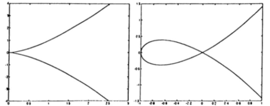
, w h ere/is a polynomial with certain coefficients from the ground field.

E x a m p le 2.2.3. The cuspidal cubic w'hich is defined by — x? =

0

is an example of a plane curve in A^.

E x a m p le 2.2.4 The nodal cubic which is defined hy — x\ — = 0 is another example of a plane curve in A^.*

Figure

2

.

2

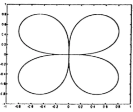
: The cuspidal cubic curve and the nodal cubic curve

E x a m p le 2.2.5. Four-leaved rose which is defined by {x\-{-x\)^— ^x\x\ = 0 is another plane curve [7, p. 146].

'T h e cuspidal cubic curve and nodal cubic curve were known by Greeks as the “cissoid of Diodes” and “conchoid of Nicomedes” and used for solving the problem of doubling the cube and trisecting the angle. Diodes showed that >^2 can be constructed by using ruler, compass and cissoid. These were the classical problems o f antiquity. Later, it was proved by Galois theory that they can not be solved by only ruler and compass construction. For more information, see [6. pp. 0-16].

Figure 2.3; Four-leaved rose

E xa m p le

2

.

2

.

6

. The twisted cubic which is defined by X

2

— = 0 and X

3

— Xj =

0

is a space curve in A^.

We will deal with the branch of a curve at a point. Before giving its defini­ tion, we prefer to give an example to be familiar with the notion.

E xam p le 2.2.7. The nodal cubic curve Xj — X| — x j = 0 has locally two components around (0,0). To see this rewrite the equation of the curve as, Xj = x i(l -h Xi), and observe that,

(1

+ x i

)^/2

=

±(1

-

1

- ix i - |x? -f ...).

This leads to the equations X

2

= xi -|- |xj — ¿Xj -f ... and X

2

= —(xi + jxJ — gxf -f ...). They are called the branches of the curve at (0,0).

We will give a precise definition of a branch by using parameterization.

Let A:[[i]] be the formal power series ring. An element ¡p of ^[[¿]] is of the form,

9

? = oq -f ai< -f- ... -f -f ... where a, € k. Order of is the degree of the smallest degree term present. Namely, smallest i satisfying a,

7

^ 0.

P ro p o s itio n

2

.

2

.

8

. A variety C of A ” has a parameterization at any one of its points (a i,...,a „ ) in the form;

Xi = <p,(i)

= ^n{t)

where (;Pi(<),..., (/?„(<) are power series in t and ((/?j(

0

) , ..., <,P„(

0

)) = (a i,...,a „ ), if and only if C is a curve.

Proof: For the part of the proof beginning with “if C is a curve", see [

1

, pp. 62-63].

Conversely, let a : f c [ x i , a ; „ ] -> C k[[t]] be the map such that a{xi) — It is obvious that that the kernel of this map is I(X). Hence,

k[x]^ ...^Xn]/ 1{ X) = Since A:[y?i(t),. . . , has dimension

1

, fc[xi,..., a :„]//(A ’) has dimension

1

, too. Hence, ^ is a curve. □

This parameterization x\ = ..., X

2

= V^n(0 ^ curve C at a point (a i,...,a „ ) corresponds to a branch of C at this point. A parameterization

x\ — ...^Xn = is redundant^ if it can be obtained from some other parameterization by substituting for t some power series in t of order >

1

. A parameterization is called irredundant if it is not redundant.

D e fin itio n 2.2.9. A branch at a point is an equivalence class of irredundant parameterizations at that point; two parameterizations are equivalent, if one can be obtained from the other by substituting a power series of order

1

, see [1, pp. 63-64].

E x a m p le

2

.

2

.

10

. For the nodal cubic curve, by using the equations

X2 = Xi + ^xf — -f ... and X2 = —(xi + + ...) obtained in Example 2.2.7, we will have two parameterizations of the curve at (0,0). The first parameterization at (

0

,

0

) is

X l = t, X2 = t + + ...,

and the second one is

Xl — C

^2

— ~ ■■■)■

PAom the definition, these are the two branches of the curve at (

0

,

0

). At ( — 1,0), the same curve has parameterizations,

Xl = —

1

, X

2

= f(i^ —

1

) and Xl = —

1

, X

2

- ■ —

1

).

They correspond to the same branch, because the second parameterization can be obtained from the first one by substituting —t which has order 1. Hence at ( —

1

,

0

), there is only one branch of the curve.

The cuspidal cubic curve has one branch at (0,0). It has the parameteriza­

tion

The twisted cubic curve has also one branch at (0,0) and it has the param­ eterization

Xl = t, X2 = X3 =

We shall deal with curves which have polynomial parameterizations. These curves can be defined by xj = x„ = (pn{i) where are polynomials in t. Not every curve does have a polynomial parameterization. But for every curve that has a polynomial parameterization, it is possible to find the defining equations, i.e., an implicit representation. (There are algorithms for doing this by using Groebner bases. For more information, see

[7, pp. 126-132].)

X\ = X2 =

2.3

Singularity

In general, singularity within a totality may be defined as a place of unique­ ness, of specialty, of degeneration, of indeterminacy or infinity, [

6

, p. 82]. Smoothness means no sudden and unexpected changes. Singularity may also be defined as the place where smoothness is violated.

For varieties, singularity can be defined both geometrically and alge­ braically. The geometric definition, which is historically the first, depends on the formal derivatives of the generators defining the ideal of that variety.

D efin ition 2.3.1. For a variety X of dimension r in A” , let /i ,...,/i t be the generators defining its ideal. X is nonsmgular at a point P G X if the rank of the matrix J = {dfifdxj{P)) is n — r. This matrix is called the Jacobian matrix at P.

From this definition, we can deduce that singular points of a curve C are those at which the curve has more than one tangent (counting multiplicity). In other words, a point of a curve is said to be singular if every line through this point has intersection multiplicity greater than

1

with the curve there.

Multiplicity of a curve at a point Pis d, if every line through Phas intersection multiplicity at least d with the curve there.

Hence, for a plane curve C of degree n, if the lines through P meet C

outside P in at most n — d points, then multiplicity of P at C is d. By using the Jacobian, a singular point of a plane curve defined by =

0

is a point ( a ,

6

) with f{a, b) =

0

,/x ,( a ,

6

) = =

0

.

E xam p le 2.3.2. Both the cuspidal cubic curve and the nodal cubic curve defined above has singularity at (0,0). These two examples arc highly illus­ trative for understanding the types of singularities. The cuspidal cubic curve which is defined by xl — x'J =

0

has cusp type of singularity at (

0

,

0

), i.e., it has the same tangent with multiplicity greater than

1

. The nodal cubic curve which is defined by Xj ~ ~ =

0

has a node at (

0

,

0

), where it has two distinct tangents.

All singular curves have either one of these two types of singularities or combinations of them.

E xa m p le 2.3.3. The four leaved rose defined by (xj T x^)^ — 4xjXj = 0 is an example having both types of singularities.

By using algebraic concepts, an equivalent definition for singularity can be found.

D efin ition 2.3.4. A local ring A with maximal ideal m is a regular local ring if dim m/m^ = dim A.

We now give an algebraic definition for singularity;

D efin ition 2.3.5. Let A” be a variety and P ^ X he & point. X is singular at P if and only if the local ring Op^x is not a regular local ring.

P r o p o s itio n 2.3.6. The geometric and algebraic definitions are equivalent. That is, for a variety X of A ” and P € X , the local ring is a regular local ring if and only if the rank of the Jacobian matrix at P for the generators of the ideal X is n — r where r is the dimension of X.

Proof. Let P £ X he (a i,...,a „). Considering P as a point of A ", the corresponding ma.ximal ideal is ap = (.xj — c j ,...,x „ — a„). A linear map a

from A = A:[xi, ...,x „] to k"' is defined by

Since a(x, — n,) = (0 ,..., 1,...,0), these form a basis for k^. Hence, the map

that а(ар) = 0. Then, it follows immediately that q' : ap/op —> is an isomorphism. Let I { X) be the ideal of X such that 1{X) = ( /i , ..,/m )· From the definition of Jacobian matrix and o r , maximum number of the independent vectors ot[fi) for i from

1

to m is the rank of the Jacobian matrix. Hence,

a { I ( X ) ) as a subspace of A:" has a dimension equal to the rank of the Jaco­ bian matrix. a' { { l { X) + ap)fap) is equal to a' {l{X)), so ( I ( X) + a‘p)/op as a subspace of apja^ has a dimension equal to the rank of the Jacobian matrix, too. Let mp be the maximal ideal of О р д . Then тр/гпр = apf { I { X) + op).

Since ap D Ц Х ) + Up

3

Up, {ap/ap)/{{ap + I { X) ) f a ‘p) is isomorphic to

ap/{ l { X) -f Op), see [13, p. 83]. Hence, dim ap f { l { X) -f Op) -f dim

{ 1( X) + ap)/op = dim ap/op — n, and dim тр/тпр -f- rank J = n. If dim

X = r, then the local ring Op^x has dimension r, too. Hence, Орд is regular if and only if dim тпр/тпр = r, which is the same thing as saying that the rank of the Jacobian matrix is n — r. This shows the equivalence of the algebraic

and geometric definitions. □

2.4

Resolution of Singularities

We can classify the singular curves by finding nonsingular curves which are birationally equivalent to these singular curves. This can be done by the reso­ lution of singularities. For curves, the construction of the blow up of the curve at a point is the main tool in the resolution of singularities of this curve.

The construction consists of simply removing the singular point and replac­ ing it by a projective line, the points of which will correspond to the tangent directions at that point. Now, let us construct the blowing up of at the point O = (

0

,

0

). The product x P’ is considered with xi,X2 affine coordi­ nates of A^ and j/i,y

2

homogeneous coordinates of PV The closed subsets of A^ X P^ are defined by the polynomials in xi, X2,yi,V2 which are homogeneous with respect to yi,t/

2

· Now, blowing up of A^ at the point 0 is defined to be the closed subset A' of A^ x P’ defined by the equation x^y2 =

3

'

2

i/i·

We have a projection map ir : X A^.

7

r"* (

0

) consists of all points of the form (

0

,

0

) x [i/i,y

2

] with [i/i,y

2

] € P’ · Hence,

7

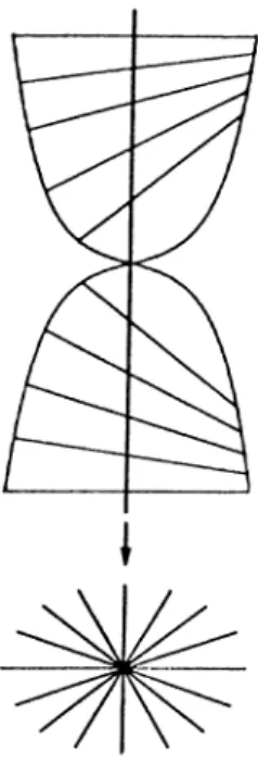
r“ ’ (

0

) is isomorphic to P’ . If we draw a picture of this blow up, it looks like a spiral staircase (Figure 2.4).

Figure 2.4; The blow up X of

We can generalize this and construct the blowing up of A ” at the point (9=(0,...,0). Now, the product A ” x is considered with affine coordinates of A " and y i , h o m o g e n e o u s coordinates of P "“ ’ . The blowing up of A " at the point 0 is defined to be the closed subset A^of A " x P’' “ ’ defined by the equations = xjyi | i , j =

1

, n} . Again, we have tt, the projection map from X to A” . x ” ’ ( 0 ) consists of all points (0 ,...,0 ) x where (yi) € P'‘ ~^ In order to find the blow up at any point, we use change of linear coordinates which sends this arbitrary point to

0

= (

0

,

If C is a curve of A" passing through 0, then blowing up of C at the point

0 is defined to be the closure C of x~^{C — 0 ) in A " x P"~* with respect to Zariski topology where tt : —» A " is the blowing up of A " at the point 0.

The map tt : (7 C is a birational morphism.

We will give illustrative examples of blow up.

E x a m p le 2.4.1. Let us find the blowing up of the nodal cubic curve

Cl : xl — Xi + Xi at 0. The blow up X of A^ at 0 is a closed subset of A^ x P’ satisfying the equation i i j

/2

= where y i,j

/2

are homogeneous coordinates. The inverse image of C\ in X will be obtained by considering this equation with the curve equation x\ = + If the open set of P’ with i/i / 0 is considered,

y\ can be set to be

1

. Then, a’j = a:j(xi +

1

) and X2 = X\y2· By substituting, we have x\yl = +

1

), from which we obtain two irreducible components, first of which is Xi =

0

,X

2

= 0 and y2 arbitrary. This is the exceptional curve

of the blow up. The other is yj =

2:1

+

1

and

12

= ^\y2·, which is the closure of

7

r“ *(C'i “ 0 ) and meets the exceptional curve at 1/2 = ±

1

, which correspond to the slopes of the two branches of Ci at 0. On the other open set, r/2

0

,

¡/2 rnay be considered to be

1

. Then, Xj = ^

1(^1

+ 1) ^nd xj = xayi- By substituting, we have Xj = x^yf + , from which we obtain two irreducible components, first of which is xi = 0, X

2

= 0 and j/i arbitrary. The other is

yj + y f x

2

= 1 and Xi = X

2

yi, which meets the exceptional curve at ±

1

. In this way, we obtained a nonsingular curve. We observe that the effect of blowing up is to separate out branches of curves passing through the singular point according to their slopes. Hence, it is clear that node type of singularities can be resolved by only one blowing up but for cusp type of singularities, this is not always the case as the following arguments show.

E x a m p le 2.4.2. Consider the cuspidal cubic curve C2 ■ x\ = x\

which is the blow up o f h? at (9, is a closed subset of x P’ satisfying the equation X\y2 = X2y\·: where y i,y

2

are homogeneous coordinates. The inverse image of C2 in X will be obtained by considering this equation with the curve equation x\ = Xj. Again if we consider the open set of P ' with y\ ^ 0,yi can be set to be

1

. Then, x\ = Xj and X

2

= Xiy2- Substitution will give

{x\y2y = Xi from which we can obtain two irreducible components first of which is xi = 0, X

2

= 0 and y2 arbitrary. Second one, which is defined by j

/2

=

3:1

and X

2

= Xiy2 is the closure of 7t~^(C2 — O). If the other open set is considered j

/2

naay be set to

1

. Then Xi = X

2

Í/

1

. By substituting, we have Xj = x^yf- We obtain again two irreducible components. X] = 0, X

2

= 0 and j/i arbitrary. The second one is X2y\ = 1 and Xi = X2y\- We again obtained a nonsingular curve.

E x a m p le 2.4.3. The last example is again a curve which has a cusp type of singularity. It is the curve Cz '· x\ = B the same procedure is followed considering the open set j/i ^

0

of P^, then the closure of n~^{Cz — 0 ) will be defined by the equations y^ = xf and y

23

^i = X2- B is obvious that the curve obtained has cusp type of singularity too. Hence, for cusp type of singularities, one blowing up may not be enough to remove the singularity. (In this example another blow up will resolve the singularity.)

It will be useful to write the equations defining the blow up in local coor­ dinates. Recalling that the blow up of X of A " at (0,...,0) is,

{ ( ( x ,....,x „ ) ,[ y i : ... :y „ ]) I x,yj - y,Xj =

0

}.

Consider =

{(/1

^ 0} C X ■ From the defining equations of the blow up we

have, X2 = _yi For x, /

0

, = f^· Define a one to one and onto map (p\ : U\ —> as,

y\ xi y\ ri

X (y, : ... ; y„l) = ( X , f a ) =

with inverse y?, ’ : A" —> f/i as,

= { X i , X i X 2 , . . . , X M X [1 :

^2

: ·.· : ^n]·

Hence, the blown up space will be considered as having local coordinates, = Xl

,^2

= If = (0 ,...,0 ) then, Xl = i

/2

= ... = y„ =

0

, and this corresponds to the point ((

0

,...,

0

),[

1

:

0

:...:

0

]) in the blown up space.

This can be done for every open set t/,.

Now, by changing to Euclidean coordinates, let us show what happens to the defining equations of the curves after the blow up in the above examples.

E xa m p le 2.4.4. Consider the nodal cubic curve defined by x\ = x\ -{■ Xj. On the open set t/j, where local coordinates are X\ = X\, X 2 = the blown up curve has the equation X j +

1

= X'^.

E xa m p le 2.4.5. For the twisted cubic curve defined by x\ = Xj, on the open set f/j, where local coordinates are X\ = x j, X

2

= th® blown up curve has the equation .Yi =

E xa m p le 2.4.6. For the last curve defined by x\ = xJ, on the open set

U\, where local coordinates are .Yj = X1. X 2 = _X\ the blown up curve has the equation X f = X|. From this equation, the blown up curve is still singular.

Hence, if we have the parameterization of a curve C as

— v^i(

0

> — v^n(O)

then the its blow up on U\ will have parameterization in local coordinates cis

(0

t[x j, l

2

, ···) ^n]/^(C) — V’iiO i •••>‘^ "(

0

]·

Then the local ring of the curve C at (

0

, 0 ,...,0 ) is

Recall that the completion of a local ring /1, denoted by A, can be defined as the inverse limit limy4/m" where m is the maximal ideal of A (see [3, pp. 100-103]). Then the completion of the local ring of the curve at (0,0, ...,0) is

^[[<^l(

0

)V^

2

(

0

) ••MV^n(

0

]]·

We have seen above that on U\ the blown up branch curve has

parameter-. . , , j * i V i 4 \ V _ *^2(0 V — Now if

ization in local coordinates diS X\ — ^i(0‘ ’

the singularity is translated to (

0

,

0

, ...,

0

), v,e have in local coordinates

where ci,C

2

,...,Cn are the constant terms of Xi, X 2-, Xn- The local ring at (

0

,

0

, . ..,

0

) is now

The completion of this local ring is

" ^1) ^7(0

^

2

, ···> ^"(<j

^11·

Chapter 3

ARF CHARACTERS OF

SINGULAR BRANCHES

In section 2.4, we have seen that for curves which have cusp type singularities, one blow up may not be enough to remove the singularity. Hence, successive resolution processes must be applied. The sequence constructed by taking the multiplicity of the singular point before each successive resolution process is called the multiplicity sequence. The problem is to obtain the multiplicity sequence from the local ring of the curve at the singularity, without applying successive blow ups to the curve. In other words, the problem is to predict algebraically the result of a geometric process.

3.1

Historical Development

The multiplicity sequence of a singular plane curve branch can be found by using Euclidean algorithm, which is the process of finding the greatest common divisor of two numbers. The branch is characterized by a number of pairs of numbers /r,, {i =

1

__ _ k) such that for i = 2,.., k is the greatest common divisor of /i,-i and t',-!, and /i, is not divisible by U{ for i = 1,...,A:. Euclidean algorithm is applied to these pairs characterizing the branch. The divisors are the multiplicities of the points of the branch and the corresponding quotients are the number of consecutive points of such multiplicity given by the divisor

[8, pp. 107-108].

curve (7, known as Puistux expansion [

6

, pp. 512-518],

X] = X

2

= ... -f- + ... + + ··· + + ... + + ...

In X

2

, m\ is the smallest exponent not divisible by u whose coefficient

6

^, is nonzero, m.2 is the smallest exponent not divisible by greatest common divisor of u and m\ whose coefficient

6^2

is nonzero, m-i is the smallest exponent not divisible by greatest common divisor of u, mi, whose coefficient

6^3

is nonzero, ..., and rrik is the smallest integer for which greatest common divisor of «, m i, m

2

, ..., rnk is

1

whose coefficient

6

^* is nonzero [

1

, p. 166]. These terms

1 ■··? ^m*^”** are the characteristic terms of the expansion. Now, we can determine pairs from the degrees of these characteristic terms, and degree of Xi, which is u. First pi = mi and t^i = u. Then for i =

2

,..., fc,

Pi = m, — m ,_i and V{ = greatest common divisor of /i,_i and i/i-j.

E x a m p le 3 .1 .1 . Consider the branch given by,

xi =

= ¿250 ^ ¿375 ^ ¿410 ^ ^417

in which only characteristic terms appear. By using the method given above, this branch is characterized by the pairs (250,100), (125,50), (35,25) and (7,5). Applying the Euclidean algorithm to these pairs,

250 = 2 X 100 + 50 100 = 2 X 50 125 = 2 X 50 4- 25 50 = 2 X 25 35 = 1 x 2 5 + 10 25 = 2 X 10 + 5 10 = 2 x 5 7 = 1 x 5 5 = 2 x 2 + 1 2 = 2 x 1

The numbers in boldface are the multiplicities, and the numbers multiplied by them in the table denote the number of times each multiplicity is repeated in the sequence. Then the multiplicity sequence of the curve branch is:

(100,100 50..50.50,50 25,25,25 10.10 5,5.5 2,2 1,1).

24

As expected, for a general curve in n-space, this method does not work. In fact the theory of algebraic curve branches in plane Wcis complete even in

1938, when Semple wrote “Singularities of Space Algebraic Curves” , see [17]. In his paper, Semple analyzed the geometry of successive resolution processes on a singular curve branch in 3-space. Semple defined proximity in order to determine a relation between the successive blow ups. A plane is obtained when a point E\ of a space curve branch is resolved. Any point E2 of is defined to be proximate to E\. By resolving E2 again, a plane is obtained. Also, a surface represents Ei — E2· These two, and e^\ meet in a line. Then from the point of view of linear equivalence, Ei = -f If E3 is chosen freely in

62

\ it will be proximate only to its immediate ancestor ^

2

, but if it is chosen in the intersection line, then it will be proximate to both Ei

and E2· Suppose, E3 is chosen from the intersection line and resolved. Then, a plane

63

^^ representing E3, a surface representing E2 — E3, and a surface representing E\ — E2 — E3. These intersect in curves, which are concurrent in a point. E4 can be chosen freely in

63

’ proximate only to .S

3

, or in the intersection of and proximate to Ei and E3, or in the intersection of

63

and Cj , proximate to E2 and E3, or as the point where the curves are concurrent, proximate to E\, E2, and E3.

We can summarize these by explaining the set up after every blow up:

(0) We have a point E\ (which is to be resolved).

(

1

) A plane is obtained. A point E2 of (1) is chosen. We have now E2

and — E2 = E\ — E2· {E2 is to be resolved.)

(

2

) We obtain a plane €2 representing E2·, and a surface e] ’ representing

El — E2· These intersect in a line. E3 is chosen on the line. Now, we have E3, — E3 = E2 — E3 and — E3 = E\ — E2 — E3. {E3 is to be resolved.)

62

(3) We obtain a plane

63

’ representing E3, a surface representing E2 —

E3, and a surface representing E\ — E2 — E3. These intersect in curves concurrent in a point.

By generalizing this, Semple defined a point Ej as proximate to Ei, if Ej

is chosen from the resolution of Ei or if Ej is any point of any diminished neighborhood of Ei, which is obtained by subtracting from it a set of points of itself. As above, E\ — Ei — E3 \s & diminished neighborhood of Ei- Hence,

E4 which is chosen from this neighborhood is proximate to E\.

£’2

— E3 is a diminished neighborhood of E2, and E4 chosen from this neighborhood is proximate to E2·

From this definition, Du Val in 1942 deduced the following three results for the n-space [8, p. 109].

(1) If a point is proximate to two others, then one of these is proximate to the other.

(2) In n dimensions, no point can be proximate to more than n others.

(3) The multiplicity of a curve in any point is the sum of its multiplicities in points proximate to that.

Du Val defined the restriction o f a point to be the number of its predecessors to which it is proximate. This led to the definition of a leading point o f the branch as one whose restriction is less than that of its successor. The sum of the multiplicities of the first n-points is called the multiplicity sum corresponding to the n-th point. Du Val called the multiplicity sum corresponding to a leading point cis a character o f the branch. His main contribution to the problem of finding the multiplicity sequence of an arbitrary curve branch is that, if the characters of the branch are known, then the multiplicity sequence of the branch can be found by applying the modified Jacobian algorithm to these characters.

The modified Jacobian algorithm [8, p. 108-109] is as follows;

We begin with the characters of an algebraic branch. They form the first row. The least of these is chosen as the divisor. The least of the remaining ones is chosen and divided by the divisor. The product (quotient x divisor for this leaist element) is subtracted from all the numbers except the divisor itself. This algorithm differs from the Jacobian algorithm by the fact that in Jacobian algorithm all the numbers in the row except the divisor are divided by the divisor so that all the remainders are less than the divisor. In modified Jacobian algorithm the remainders may be greater than the divisor. The divisor and the remainders obtained form the second row. If any remainder is zero, it is omitted. The algorithm stops, when we reach a row consisting of only one element. The divisors are the multiplicities of the points of the branch, and the quotient corresponding to each divisor is the number of points of the corresponding multiplicity.

E xa m p le 3.1.2. We will apply the modified Jacobian algorithm to two algebraic curve branches. The first one has the characters 100, 250, 425, 485, 512. The second one is an example of Du Val which has the characters 2087, 4610, 6068, 6384.

100 100 50 50 425 485 512 _{1 2} 1 2087 4610 6068 6384 _{1 2} 200 200 200 _{1 1} 4174 4174 4174 ₁ 225 285 312 _{1 2} 1 2087 436 1894 2210 _{1 4} 100 100 100 ₁ 1744 1744 1744 ₁ 125 185 212 _{1 2} 343 436 150 466 _{1 2} 100 100 100 ₁ 300 300 300 ₁ 25 85 112 _{1 2} 43 136 150 166 _{1 3} 50 M 1 129 129 129 1 25 35 62 _{1 1} 43 7 21 37 _{1 3} 25 25 1 21 21 21 1 25 10 37 _{1 2} 22 7 16 _{1 2} 20 20 ₁ 14 14 ₁ 5 10 17 _{1 2} 8 7 2 _{1 3} 15 1 6 6 1 5 7 _{1 1 1} 2 1 2 _{1 2} 5 _{1 1} 2 2 ₁ 5 2 _{1 2 1} 1 ₁ 4 _{1 1 1} 1 2 _{1 2 1 1} % _{1 1 1} 1 _{1 1 1}

The multiplicity sequence of the curve branch, which ha^ the characters 100, 250, 425, 485, 512 is:

(100,100 50,50,50,50 25,25,25 10,10 5,5,5 2,2 1,1).

The multiplicity sequence of the curve branch, which has the characters 2087, 4610, 6068, 6384 is:

(2087,2087 436,436,436,436 150,150 43,43,43 7,7,7,7,7 2,2,2 1,1)

Every time a column enters the algorithm, a leading point is passed so restriction rises by unity. Every time a column becomes zero, restriction falls by unity. We can observe from the table that, for the first curve branch, the restriction can not be greater than 2. Thus, the branch is capable of existing in two dimensions. This is the expected result because the example given previously as a plane algebraic curve has the same multiplicity sequence. For

the second curve, the restriction rises to 3. Hence, the branch is capable of existing in three dimensions, but not in a plane.

This method is valid for any algebraic curve branch with known characters. More than this, it gives us the opportunity to know the minimum dimension in which the branch is capable of existing. What Du Val aisked was, how we should obtain the characters of the curve branch. The relation between these and the expansion of branch in power series was unsolved, until Arf wrote his paper in 1949 [2].

3.2

Arf Rings, Closure and Characters

A rf’s work depends on the observation that there is an algebra behind these geometric arguments. He shows that the multiplicity sequence of an algebraic branch can be defined by purely algebraic notions. He constructs the link between geometry and algebra by showing that the completion of the local ring at the singularity of the branch carries all the information necessary to obtain the multiplicity sequence.

For a curve branch having the parameterization X\ = <p\{t)·, ...,in = the completion of the local ring is ..., </?„(<)]], i.e., the ring formed by all formal series of the form,

E

•V^n"

«1, ■••,«n>0

where a,. e k .

Arf passes from geometry to algebra by using the completion of the local ring. He constructs the canonical closure of this ring, later called the A rf closure. The orders of the elements of the constructed ring form a semigroup. This is passing from algebra to arithmetic. Now from this semigroup, Arf obtains some numbers by a process to be described below, and then applies the modified Jacobian algorithm to these numbers to obtain the multiplicity sequence.

In this way, he provides an answer to the question of finding the relation that must exist between Du Val's results and the series representation of the branch.