EfFEII IF EMil^SE SI IT 5Ш?£!0Ш
. 4 \i4' * / '^ai'· if· Ѵл'Λ,ί
EFFECT OF EXERCISE ON QT DISPERSION
A THESIS
SUBMITTED TO THE DEPARTMENT OF ELECTRICAL AND
ELECTRONICS ENGINEERING
AND THE INSTITUTE OF ENGINEERING AND SCIENCES
OF BILKENT UNIVERSITY
IN PARTIAL FULFILLMENT OF THE REQUIREMENTS
FOR THE DEGREE OF
MASTER OF SCIENCE
By
Liitfii Ozçakir
December 1998
1 4 ^ ί I ^ и и
11
I certify th at I have read this thesis and th at in my opinion it is fully adequate,
in scope and in quality, as a thesis for the degree of Master of Science.
Prof. Dr. Hefyrettin Köyrnen (Supervisor)
I certify th at I have read this thesis and that in my opinion it is fully adequate,
in scope and in quality, as a thesis for the degree of Master of Science.
o f. Ziya iIder
I certify th at I have read this thesis and that in my opinion it is fully adequate,
in scope and in quality, as a thesis for the degree of Master of Science. /'!
' ( /
I ■
Prof. Dr. Enis Çetin
Approved for the Institute of Engineering and Sciences:
Prof. Dr. Mehmet Balpay
ABSTRACT
EFFECT OF EXERCISE ON QT DISPERSION
Lütfü Özçakır
M.S. in Electrical and Electronics Engineering
Supervisor: Prof. Dr. Hayrettin Köymen
December 1998
Electrocardiogram (ECG) is the measurement of potential differences oc curring on the body due to the currents th at flow on the heart during diastole and systole. Cardiac abnormalities cause uncommon current flows, leading to strange waveform morphologies in the recorded ECG. Since some abnormalities become visible in ECG only during activity, exercise ECG tests are conducted.
Among all abnormalities, exercise induced ischemia is considered in this study. The previous studies have shown that exercise induced ischemia increases the QT dispersion (QTD).
The patients in this study have been validated by cardiologists using ST segment analysis. However, the sensitivity and specifity of ST segment analysis is low. Some of the patients have been validated as ischemic using the coronary angiography results.
A different method to measure the QT interval through out the exercise ECG test has been developed . The algorithm is designed to cope with the artifacts of exercise ECG. Such as high noise level and PT fusion. A different approach to obtain the QTD has been developed.We have shown that, QTD increases signiflcantly in patients who have ischemia during exercise. The sen sitivity and specifity of exercise ECG test can be increased if QTD analysis is used as an additional tool to ST analysis.
Keywords : Exercise ECG, QT interval,QT Dispersion
ÖZET
EFORUN QT BOZULUMU ÜZERİNE ETKİSİ
Lütfü Ozçakır
Elektrik ve Elektronik Mühendisliği Bölümü Yüksek Lisans
Tez Yöneticisi: Prof. Dr. Hayrettin Köymen
Aralık 1998
Elektrokardiyogram (EKG), kalpten sistol ve diyastol sırasında yayılan elektrik akımlarının vücudun yüzeyinde oluşturduğu potansiyel farkların ölçümüdür. Kardiyolojik bozukluklar EKG’de normal olmayan morfolo jilere neden olurlar. Bu anormalilerden bazıları sadece aktivite sırasında gözlenebildiği için Eforlu EKG Testi uygulanmaktadır.
Bu çalişmada, bütün bu kardiyolojik bozuklukların arasından efor ile oluşan iskemi göz önüne alınacaktır. Daha önceki çalışmalar, efor ile oluşan iskeminin QT bozulumunu (QTB) arttırdığını göstermişlerdir.
Bu çalışmadaki hastalar, ST aralığı analizi kullanılarak, kardiyologlar tarafından onaylanmışlardır. Ancak ST aralığı analizinin hassasiyeti ve ayırıcılığı düşüktür. Buna ilaveten, bazı hastalar koroner anjiyografi sonuçları kullanılarak iskemik olarak onaylanmışlardır.
Bütün eforlu EKG testi sırasında QT aralığını ölçmek için, farklı ve yeni bir metod geliştirilmiştir. Algoritma eforlu EKG bozuklukları ile başa çıkabilecek şekilde tasarımlanmıştır. Yüksek gürültü seviyesi ve PT birleşimi bu bozukluklara örnektir. Ayrıca QTB’yi elde etmek için farklı bir yaklaşım sunulmuştur.QTB’nin aktivite sırasında iskemisi olan hastalarda dikkate değer bir şekilde arttığını gösterdik. Eğer, QTB analizi, ST aralığı analizine ek bir araç olarak kullanılırsa, eforlu EKG testinin hassasiyeti ve ayırıcılığı arttırılabilir.
Anahtar Kelimeler : Eforlu EKG, QT aralığı, QT bozulumu.
ACKNOWLEDGMENTS
I would like to express my sincere gratitude to Dr. Hayrettin Köymen for his supervision, guidance, suggestions, encouragement through the development of this thesis.
I would like to thank to Dr. Enis Çetin and Dr. Ziya İder for reading the manuscript and commenting on the thesis.
I am indebted to Kürşad Tüzer and Mustafa Solmaz from Kardiosis Ltd. Co. and Ibni Sina Hospital Exercise ECG Dept, personnel for their assistance in data acquisition; to Dr. Sadi Güleç for the analysis of the results and to Dr. Olcay Taşdemir for her partnership.
Special thanks are due to Dr. Orhan Arikan for his suggestions. I would like to express my appreciation to Burak Acar, Mehmet Alpata and to all of my friends in the department, whose names would make a very long list, for their continuous support through the development of this thesis. Finally, I would like to thank to my parents, brother and my wife , whose understanding made this study possible.
C ontents
1 Introduction 1
1.1 Objective of the study 1
1.2 O u tlin e... 5
2 A Review on Exercise ECG and QT Dispersion 7 2.1 Exercise Electrocardiography 7 2.2 Definition of the End of the QT I n t e r v a l ... 11
2.3 Clinical Value of QT D isp ersio n ... 12
2.4 Exercise and Ventricular Repolarization... 13
3 Methods 15 3.1 D ata A c q u is itio n ... 15
3.2 Obtaining Heart Rate T r e n d ... 17
3.2.1 Recognition of QRS C o m p le x e s... 17
3.3 Obtaining the Average B e a ts... 20
11
«·
3.3.2 Averaging the Beats 21
3.4 Measuring the P a ra m e te rs ... 24
3.4.1 Detecting the Q Point and T Peak 25
3.5 Detecting the T wave end 30
3.6 Checks for Eliminating the T Waves and M easurem ents... 34
3.6.1 Cross Correlation Coefficient Check,(CCCC) 34
3.6.2 Amplitude, PT Fusion and Energy C h e c k s ... 35
3.6.3 Post-measurement C h e c k s ... 36
4 Statistical Evaluation 39
4.1 Statistical E lim in a tio n ... 39
4.2 Finding the Lead Pairs Giving the Maximum Q T D ... 42
4.2.1 Steps to Obtain QT Dispersion T re n d ... 44
5 Results and Conclusions 46
5.1 Future W o rk ... 54
List o f Figures
1.1 QT dispersion d e fin itio n ... 3
2.1 Standard leads used in ECG recording 8 2.2 Typical heart beat 8 2.3 Typical beats r e c o r d e d ... 9
2.4 Typical beats re c o rd e d ... 10
2.5 Different T wave end definitions 1.nadir between T wave and U waves 2. intersection of tangent line with baseline 3.return of polarization to isoelectric l i n e ... 12
2.6 PT fused beats for leads D1 and D 2 ... 13
2.7 PT fused beats for leads V4 and V 5 ... 14
3.1 Block Diagram of the a lg o rith m ... 16
3.2 RR tachogram showing the detection errors 19 3.3 20 Hz filter block d i a g r a m ... 20
3.4 20 Hz filter frequency response... 21
3.5 Average beat at r e s t ... 22
IV
3.6 Average beat at peak e x e rc is e ... 23
3.7 Baseline Correction of the beat 24 3.8 The average beat and its d e riv a tiv e ... 25
3.9 Various T wave morphologies [1], 27 3.10 T wave peak search window 29 3.11 The T wave end detection visually... 30
3.12 The window of parabola fit and parabola fitted to T wave peak 32 3.13 The parabola window, parabola and tangential l i n e ... 33
3.14 The parabola window, parabola and tangential line for PT fused b e a t ... 34
3.15 The T wave test Block D ia g ra m ... 38
4.1 QT intervals and parabola fit to V 3 ... 40
4.2 QT intervals and parabola fit to D 2 ... 41
4.3 QTD trends obtained by classical and our a p p ro a c h ... 43
4.4 QTD vectors for five maximum mean v a l u e s ... 44
5.1 QTD and Heart Rate ST=- Q T=- A = ? ... 47
5.2 QTD and Heart Rate S T = + Q T = + A = + ... 48
5.3 QTD and Heart Rate S T = + Q T = + A = + ... 49
5.4 QTD and Heart Rate S T = + Q T = + A=? 50 5.5 QTD and Heart Rate S T = + Q T = + E X T A = + ... 51
V
5.7 QTD and Heart Rate S T = + Q T=-
A=-A.l QTD and Heart Rate for patient 3038 ST=- Q T=- A=?
53 r= - A=? 56 r= - A=? 56 r=- A=? 57 T = - A=? . . . . 57 ?=- A=? 58 ?=- A=? 58 :=- A=? 59 A=? 59 A=? 60 A=? 60 =- A=? 61 =- A=? 61 ’=- A=? 62 ’=- A=? 63 A=? 63 '=- A=? 64 =- A=? 64 =- A=? 65 =- A=? 65 =- A=? 66
VI
A.22 QTD and Heart Rate for patient 5 ST=- Q T=- A —? 67
A.23 QTD and Heart Rate for patient 6 ST=- Q T=- A=? 67
A.24 QTD and Heart Rate for patient 8 ST=- QT=- A=? 68
A.25 QTD and Heart Rate for patient 9 ST=- Q T=- A=? 68
A.26 QTD and Heart Rate for patient 10 ST=- Q T=- A = ? ... 69
A.27 QTD and Heart Rate for patient 11 ST=- Q T=- A = ? ... 69
A.28 QTD and Heart Rate for patient 12 ST=- Q T=- A = ? ... 70
A.29 QTD and Heart Rate for patient 113 ST=- QT=- A = ? ... 70
A.30 QTD and Heart Rate for patient 13 ST=- Q T=- A = ? ... 71
A.31 QTD and Heart Rate for patient 14 ST=- Q T=- A = ? ... 71
A.32 QTD and Heart Rate for patient 15 ST=- Q T=- A = ? ... 72
A.33 QTD and Heart Rate for patient 18 ST=- Q T=- A = ? ... 72
A.34 QTD and Heart Rate for patient 17 ST=- Q T=- A = ? ... 73
A.35 QTD and Heart Rate for patient 20 ST=- QT=- A = ? ... 73
A.36 QTD and Heart Rate for patient 21 ST=- QT=- A = ? ... 74
A.37 QTD and Heart Rate for patient 24 ST=- Q T=- A = ? ... 74
A.38 QTD and Heart Rate for patient 25 ST=- Q T=- A = ? ... 75
A.39 QTD and Heart Rate for patient 23 ST=- QT=- A = ? ... 75
A.40 QTD and Heart Rate for patient 32 ST=- QT=- A = ? ... 76
A.21 QTD and Heart Rate for patient 3084 ST=- Q T=- A=? 66 A.41 QTD and Heart Rate for patient 35 ST=- Q T=- A = ? ... 76
V l l
A.43 QTD and Heart Rate for patient 39 ST=- QT=- A —7 ... 77
A.44 QTD and Heart Rate for patient 38 ST=- Q T=- A = ? ... 78
A.45 QTD and Heart Rate for patient 42 ST=- QT=- A = ? ... 78
A.46 QTD and Heart Rate for patient 40 ST=- Q T=- A = ? ... 79
A.47 QTD and Heart Rate for patient 41 ST=- QT=- A = ? ... 79
A.48 QTD and Heart Rate for patient 44 ST=- Q T=- A = ? ... 80
A.49 QTD and Heart Rate for patient 46 ST=- Q T=- A = ? ... 80
A.50 QTD and Heart Rate for patient 48 ST=- Q T=- A = ? ... 81
A.51 QTD and Heart Rate for patient 52 ST=- Q T=- A = ? ... 81
A.52 QTD and Heart Rate for patient 53 ST=- QT=- A = ? ... 82
A.53 QTD and Heart Rate for patient 54 ST=- QT=- A = ? ... 82
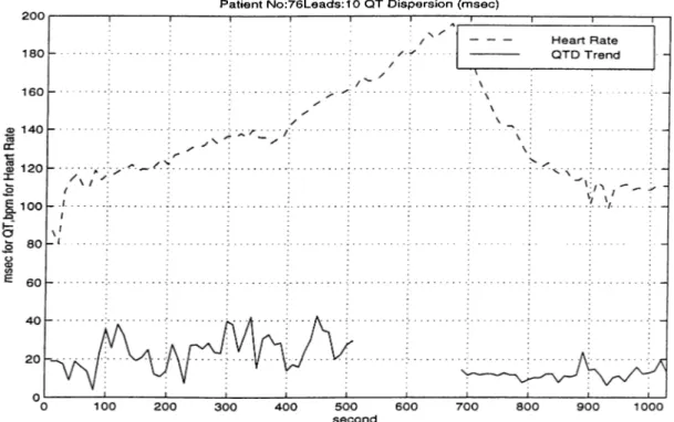
A.54 QTD and Heart Rate for patient 76 ST=- Q T=- A = ? ... 83
A.55 QTD and Heart Rate for patient 59 ST=- Q T=- A = ? ... 84
A.56 QTD and Heart Rate for patient 58 ST=- Q T=- A = ? ... 84
A.57 QTD and Heart Rate for patient 60 ST=- Q T=- A = ? ... 85
A.58 QTD and Heart Rate for patient 62 ST=- Q T=- A = ? ... 85
A.59 QTD and Heart Rate for patient 61 ST=- QT=- A = ? ... 86
A.60 QTD and Heart Rate for patient 63 ST=- QT=- A = ? ... 86
A.61 QTD and Heart Rate for patient 64 ST=- QT=- A = ? ... 87
A.42 QTD and Heart Rate for patient 34 ST=:- Q T=- A = ? ... 77
V l l l
A.65 QTD and Heart Rate for patient 3083 S T = + Q T = + A=? 89
A.66 QTD and Heart Rate for patient 16 S T = + Q T = + A = ? ... 89
A.67 QTD and Heart Rate for patient 37 S T = + Q T = + A = ? ... 90
A.68 QTD and Heart Rate for patient 49 S T = + , E X T ... 90
A.69 QTD and Heart Rate for patient 3062 S T = + , E X T ... 91
A.70 QTD and Heart Rate for patient 3071 S T = + , E X T ... 91
A.71 QTD and Heart Rate for patient 3078 S T = + , E X T ... 92
A.72 QTD and Heart Rate for patient 3087 S T = + , E X T ... 92
A.73 QTD and Heart Rate for patient 27 S T = + , E X T ... 93
A.74 QTD and Heart Rate for patient 28 S T = + , E X T ... 93
A.75 QTD and Heart Rate for patient 3032 ST=- Q T = + A=? . . . . 94
A.76 QTD and Heart Rate for patient 3034 ST=- Q T = + A=? . . . . 94
A.77 QTD and Heart Rate for patient 3037 ST=- Q T = + A=? . . . . 95
A.78 QTD and Heart Rate for patient 3077 ST=- Q T = + A=? . . . . 95
A.79 QTD and Heart Rate for patient 3080 ST=- Q T = + A=? . . . . 96
A.80 QTD and Heart Rate for patient 3081 ST=- Q T = + A=? . . . . 96
A.81 QTD and Heart Rate for patient 31 ST=- Q T = + A = ? ... 97
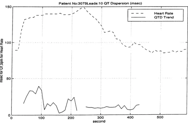
A.63 QTD and Heart Rate for patient 3044 S T = + Q T = + A = + . . . 88
A.64 QTD and Heart Rate for patient 30 S T = + Q T = + A = + . . . . 88
A.82 QTD and Heart Rate for patient 3068 S T = + Q T=- A=- . . . . 97
IX
A.84 QTD and Heart Rate for patient 3072 S T = + Q T=- A=?
A.85 QTD and Heart Rate for patient 19 S T = + Q T=- A=?
98
99
A.86 QTD and Heart Rate for patient 43 S T = + Q T=- A=? 99
List of Tables
2.1 Bruce Protocol S t e p s ... 11
Chapter 1
Introduction
1.1
Objective of the study
The diagnosis of coronary artery disease (CAD) in subjects with chest pain is a difficult problem in clinical medicine. Exercise ECG testing has a limited value in the detection of CAD (especially in female population) due to excessive false positive results [2]. Depending on disease prognosis, the false positive rate changes from % 25 to % 50 in patients with typical chest pain [3].
The QT interval is the interval from the beginning of ventricular depolar ization (Q point in the ECG) to the end of the ventricular repolarization (end of the T wave) and is sensitive to myocardial ischemia. The interlead vari ation in the 12-lead (or the measured leads) is called QT dispersion (QTD). QTD reflects the inhomogenity in the duration of myocardial repolarization and is increased in patients who have ischemic heart disease and myocardial infarction.
Numerous investigations are being done for the identification of the pa tients at risk of sudden cardiac death. Most of the sudden deaths are due to ventricular tachycardia or ventricular fibrillation.
If a part, of the heart can not get enougli l)loo(l diu' to narrowc'd artc'iies: this [)art has been injured or dead. The heart i.s than caJhid to have, i.sv.hc.mm. These injured or dead parts can not giv(! eiiougli (d(!ctrica.l ri'sponsi' i,o hor mones which stimulate the heart to beat fast(!r during (!X(!rcise as wcdl as tlu' healthy parts [4]. This phenomenon causes diflerent timing of nipolarization between healthy and injured {)arts. Different timing of r(i[)ola.rization betwoHui neighboring· areas of the heart causois ventricular arrhythmia by allowing cur- r(uit eddies and reentrant tachy(;ardia via microcircuits within tlu; ventrichi. Nonuniform myocardial repolarizatiori time may result from iiihomogcuiity of a,ction potential duration due to slow conduction or altercnl conduction pa.th- ways through the heart [5]. Assessment of this inhomognnity should lx; done using the standard 12-lead ECG’s fiducial points like (,^,T.
The maximum QT interval should be measured from the beginning of the QRS complex to the end of the latest T wave among all leads of a simultaneous 12-lead EGG recording. This approximates the time from the earliest depo larization of ventricular myocardium to its latest repolarizatioii. Beginning of the QRS complex is approximately the Sc^rne for all leads thus measuring the T waves’ end is important. The QT interval has long been known to vary significantly between the individual leads of the 12 lead EGG, [G] but in 1990 a potential application of this interlead difference was proposed by Day et al. [4]. These authors suggested that if individual leads reflect the regional activity, the interlead difference in QT interval may provide a measure of repolarization inhornogenity. They called this interlead difference as QT Dispersion. Fig ure 1.1 shows this definition. The time interval between last 2 vertical lines shows QT Dispersion definition. The spikes show Q point , S point, J point, beginning of T wave, T peak and end of T wave respectively.
In most studies [7], QT dispersion has been defined as the difference be tween the maximum and minimum QT intervals measured from each of the 12 standard leads. However the standard deviation (SD) of C^T intervals may provide a more reliable measure of dispersion since it does not depend on the number of leads measured. Hanakova [8] found that the SD of the C^T interval is less effected by the number of the missing leads.
Since the QT interval shortens as the heart rate increases, nuiiK'rous for
Q T Dispersion for 12 leads
Figure 1.1; QT dispersion definition
and compare the measurements, which have been done at different fieart rates. Tliese formulas are assumed to correct the QT interval with respect to heart rate. The frequently used formulas are Bazett’s formula [9] and Framingham Heart Study QT interval correcting formula [10]. The corrected measurements are shown as QTc- Equations 1.1 and 1.2 shows B azett’s and Framingham correcting formulas respectively.
QTc = QT + QT
V RRint
QTc = QT + 0.154(1 - RE.)
(1.1)
(1.2)
These formulas are derived for heart rates less than 120 l)i)m, hence it is not appropriate to use them for exercise ECG. Thus in this study no comment has b(ien done on corrected QT Dispersion [10]. These calculations may lead to
iucrensed QT^ dispersion during liigh(!r iniart rai.cis and inliiumci' the diagnosis made for the patients who have a higher lieart ra,te due to ilhi(!ss.
(,^T dispersion provides a riKiasure of arrhytlimia risk too [10]. Thus it ca.ii he used to detect the patients who will have arrliytlimia during (ixerciscc
The exercise ECG test records used in this study have hemi n-ad i)v the cardiologists in the hospital. They have validated the records using ST siigiiient analysis. In our research an exercise test is dia.gnos(id as POSITIVE by the cardiologist if a ST segment depression > 1mm occurs in 3 consecutive beats, in 2 leads at least. Also the other parameters such as agig sex and history are considered. The diagnosis of exercise tests is done by cardiologists in Ibni Sina Hos[)ital, Cardiology Dept. Some of the patients who have a jKisitive exercise ECG test had undergone coronary angiography to make tliii liiial diagnosis about the coronary arteries.
Cuinming et. al [11] reported that ST segnumt changes in % 25 to % 66 of women confuses the interpretation of routine treadmill exercise test. The sensitivity and specifity of treadmill exercise test when diagnosing the ischemic heart disease is not high if we use only the ST segment changes.
Our hypothesis is that exercise-induced myocardial ischemia can increase (,^T interval in the regions of ischemia and give rise to an increase in QTD in the 12-lead ECG. The QTD analysis can improve the diagnostic accuracy of exercise ECG test when used with ST segment analysis. Sinc:e it is known that exercise induces ischemia in the heart, assessing the QT dispersion during exercise can give useful information for the diagnosis of ischemic heart disease.
A different approach and algorithm for the measurement of QT interval a,nd formation of QT dispersion are proposed in order to reduce the effects of measurement errors in the analysis. The QT interval measurements have been done throughout the whole exercise test. The formation of the QTD is a,Iso different from previous approaches. The artefacts are exercise specific such as T-P wave fusion, muscle noise (EMG) and baseline wander (electrode movement). The algorithm was designed to cope with these artefacts. This algorithm is immune to noise and PT fusion. The proposed method is designed to run in real time and can be installed into a real-time ECG machine program
The fiducial points found by the algorithm are visually verified. During ver ification, the computer program of Massachiites Institute of T(!clmology (.MIT) and Beth Israel Hospital (BIH) has been used. All of the beats are vi(iwed by this i)rograrn. The algorithms are improved as a result of vtuification.
VVe have seen that QT dispersion increases signific:a.utly in patients with ischemic heart disease (approved by coronary angiography results for some [)atients) and decreases in patients who had drug or surgical therapy such as Pcnfusiorial Transluminal Coronary Angioplasty (PTCA) and stent. These are two methods to reperfuse the veins and decreases the level of ischemia.
easily without eifcictirig the operation of program.
1.2 Outline
In this study the effect of exercise induced ischemia on QT dispersion is inves tigated during a standardized exercise ECG test.
Chapter 2 presents a review on exercise electrocardiography followed by the description of previous studies and clinical value of the QT dispersion.
In Chapter 3, the methods and materials used in this study are i)resented. First a section on data acquisition and QRS complex detection is presented. N(!xt, composing average beats, filtering, finding the fiducial points is dis cussed. Measuring the QT interval and elimination of the measurements are also discussed in this chapter.
In Chapter 4 the statistical elimination and process of the measurements are discussed. The difference of the study from the previous studies has been shown here.
In Chapter 5 we present the results of the study. We describe the patient set and present the QT dispersion plots of these patients. Also conclusions have been made on these patients. As the last step a short section for the future study is presented.
A CDROM including all the related softwani a.nd data has Ihh'u i)repan'd. The flowchart of the whole algorithm is pn^sented in cha,pt(u· 3. In Appcnidix A, the plots of QT dispersion i)lots for all i)ati(!iits hav(' hecui given.
Chapter 2
A R eview on Exercise ECG and
QT D ispersion
2.1 Exercise Electrocardiography
ECG is the recorded electrical potential generated h.y tin; heart during a cardiac cycle. An electrical impulse passes through the tissues causing small amount of electrical currents spreading all the way to the surface of the l)ody. These currents generate the electrical potentials recorded in ECG. Figure 2.1 shows the location of the ECG recording leads on the body.
The normal ECG is composed of a P wave, a QRS complex and a T wave. QRS complex is actually three separate waves, the Q, R, and S waves. .1 point is end of the QRS complex. All of them are caused by the deijolarization of the ventricles when the impulse is propagating. T wave is a rc'siilt of rei)olarization of the ventricles. Before a new depolarization of ventricles start, rei)olarization must end. In other words the T wave peak is always before the Q point of new corning beat. This is a physical fact and will be used while defining T wave peak search window.
Figure 2.1: Standard leads used in ECG recording
Figures 2.2 and 2.3 show typical heart beats recorded from standard 12-lead channels.
A ty p ic a l h e a r t b e a t r e c o r d e d
The exercise electrocardiography (stress ECG test or exercise ECG tt is one of the most important non-invasive diagnostic tests in the clinical eval uation and management of patients with cardiovascidar disease, particularly coronary artery disease or ischemic heart disease. The ex(;rcise ECG test is in'imarily used for the assessment of the chest pain and for the early detection
of the coronary artery disease. Ischiirnia is caused due to d(!cr(!ased blood (low to inyocardia from the heart arteries. Heart arteries are called ’’Coronaries’’
In addition, the exercise ECG test can provid(! valuahk! information in eval uating the capacity of the patients with CAD, also in ('valuating tlu! efficiency of medical or surgical therapy [12].
Figure 2.3: Typical beats recorded
Exercise protocols have been developed by different investigators for the exercise ECG test using either a treadmill or a bicycle ergometer. The follow ing are valuable contributors of modern exercise ECG: Astrand, Balke, Black burn, Bruce, Clausen, Ellestad, Epstein, Fox, Froelicher, Kattus, McHenry, Naughton, Sheffield and many others [12]. In 1956 modern exercise ECG tests
10
using motor driven treadmill began to receive vvid(i acceptance lor r(!S(iarch pur poses as well as clinical medicine. At present the treadmill is tlui most popular method of exercise testing.
Although various exercise protocols are desigiuHl by different invcistigators, none of these are ideal and can be modified for special i)urposes. In some l)iotocols, the work load is increased by changing the speed at a hx(Ml inclination (Astrand) where as in others the incline is increas(id while si)eed is hxcxl. The workloads should be increased gradually and maintained for a sufficient length of time to achieve a near physiological state.
Figure 2.4: Typical beats recorded
In Bruce protocol both the speed and inclination is increased every three minutes in each of the seven stages. It is relatively short in duration but has the disadvantage of having very heavy exercise workloads for cardiac patients
l i
or elderly individuals. Table 2.1 shows the steps of the Brucc' protocol. In this study all patients had undergone a Bruce protocol (ix(ncis(' ECG t('st.
Stage Grade 10 12 14 16 18 20 22 Speed (krn/h) 2.8 4.2 5.6 6.8 8.3 9.1 10 Total TiiiKi 6 1 2 15 18 21
Table 2.1; Bruce Protocol Steps
2.2 Definition of the End of the QT Interval
Definitions of the end QT interval vary between studies [5]. Definitions are: 1. the return of T wave to isoelectric line,
2 . the nadir between the T wave and the following U wave, and
3. the intersection of a tangent line to the downslope of the inajor repolariza tion wave (T wave) with the baseline.
Figure 2.5 shows different T wave end definitions and the process done by the cardiologists to detect the T wave end.
It is very difficult to see the U wave in exercise ECG because the signal to noise ratio (SNR) is low. The effect and the cause of the U wavois are not very clear so the second definition is not used in this thesis. VVe eliminate the first definition because very high heart rates are considered in this study. T wave’s return to baseline is not seen since a PT fusion occurs. VVe have used the third definition, which gave the best results since it uses Least Sejuares approximations while fitting the tangent line to the downsloping part of T wave.
The relationship between QT Dispersions measured using different defini tions for the end of the QT interval is unclear. Kautzner et. al. [13] have shown
12
Figure 2.5: Different T wave end definitions 1.nadir between T wave and U waves 2. intersection of tangent line with baseline S.return of polarization to isoelectric line
correlates poorly with that derived from QT intervals where the end of the QT interval is defined as the return of the T wave to the isoelectric line.
2.3 Clinical Value of QT Dispersion
Interpretation of results obtained from studies about QT Dispersion is not stan dardized in clinical practice since different methods are used. In some studies the clinical value of QTD will depend on its ability to predict arrhythmogene- sis. In this thesis we have used the QTD to predict the ischemic heart disease (IHD). Remember that ischemia is a result of CAD. QTD increases reversibly during ischemia in patients with CAD. Ischemia occurs due to exercise or drugs such as dipyridapiole and dobutamine [14]. Contrary to this, QTD decreases
13
such as dipyridamole and dobutarnine [14]. Contrary to tliis, C^TD d(;cr('as(\s or remains constant during· exercise in healthy subjc'cts. During acute' myocar dial infarction QTD is very high in early days of infarction a.nd d(H:i(!a.ses a,s reperfusion starts [15].
Liset N. et. al. [7] showoid that the s[)ecifity ot (cxe'rcise ECG test for vvoiikui increases up to % 100 if QTD is used as an additional diagnostic tool with ST analysis. They have measured the QT interval visually and usíkI the standard definitions to form the QTD.
2.4 Exercise and Ventricular Repolarization
PT lusion on D1
Figure 2.6: PT fused beats for leads D1 and D2
Exercise is a useful non-invasive method to produce variations in heart rate, causing dynamic changes in QTD. During exercise, dynamic parameters of the heart can be examined. It may cause arrhythmia and sudden death causing ischemia in patients with CAD. Mecisuring changes in QT interval (not QTD) during exercise was investigated to discriminate ischemic patients from nonischemic patients [16].
The exercise induced QT shortening depends on not only to the iiu:rease in heart rate but also on the level of catecholamine activity (such as adrenalin).
14
Figure 2.7: PT fused beats for leads V4 and V5
The response of ischemic myocardium to catecholamines in the blood is dif ferent than the non-ischernic myocardium which may cause the QT interval in ischemic myocardium to be longer. 12 lead ECG sees the different parts of the myocardium so the leads that are near to the ischemic myocardium will reveal a longer QT interval causing QTD to increase.
It has been shown that antiarrhythmic drug therapy (beta-l)locker) and PTCA (an invasive method to reperfuse the ischemic myocardium) can decrease the QTD in ischemic patients during exercise [4].
Since the body needs more blood during exercise, the heart beats faster. As the heart rate increases a new depolarization of atriums occurs before all the ventricle muscles fully repolarized. This causes a PT fused beat and is one of the main problems while measuring the T wave end.
VVe can see T waves in some leads during exercise, which we do not see at rest, or some T waves can be lost during exercise. The morphology of T wave can change very much in some patients during exercise. In this case we need to update some of the algorithm parameters as the exercise i)rogress.
Figures 2.6 and 2.7 shows the PT fused beats for D1,D2 and V4,V5. As seen in these figures the P wave of the beat at the right is under the T wave of the beat at the left. Thus it can not be seen.
Chapter 3
M ethods
3.1 Data Acquisition
The electric field created by the heart propagates throughout the body and can be measured on its surface. The potentials are measured by placing electrodes to locations on the body. These signals are recorded as EGG data.
Exercise EGG test data recordings for this study were taken out in Ankara University, School of Medicine, Ibni Sina Hospital Gardiology Dei)artment. VVe have used a Kardiosis PG based exercise EGG system to record the data. 12 lead EGGs were recorded to harddisk during Bruce Protocol I)ased exercise test with 500 sec at 2.9 microvolt resolution. 89 exercise EGG test data are used for the study. The duration of the records vary from 5 Min. to 20 Min. The complete block diagram of the algorithm is shown in figure .3.1.
IG
17
3.2
Obtaining Heart Rate Trend
C.^T interval measurements have i)eeii doiui on tiitui av(ir;vf:,(!(l EC'G eompli'xcis. In order to obtain the time aviiraged EGG eomphixcis we lUH'd th(i lu'art ra,t(' trcuid. VVe have to know the places of the R waviis on tin; roH-.ord (exactly. R wave was chosen as the alignment point for ;iv(iraging since it is (easier to detect. Also we will use this information to inv(!stigat(' the rehitioii betweiui (,^T interval and heart rate trend.
Recorded data files during exercise have the extension of .EXR. 73 charac ters from the beginning of tluise EXR fihis contain tin; information a.bout the subject. Following 73 characters, standard 12 lead EGG record is found. Leads are recorded one after another using 2 byte integers for each samphe Also a 30 second rest EGG data is recorded with the extension .RES when the patient is standing. We have recorded these raw data to GD-R.OM for future usage.
R.R, interval tachograms are extracted by identifying the R. waves through the record. We make this identification using a ternplatii-matching algorithm. This algorithm is based on calculation of Gross Gorrelation Goefficient (GGG) between the composite EGG signal and a template i)roduced from the EGG
3.2.1 Recognition of QRS Complexes
The rest and exercise EGGs are combined and a file with the (extension COM.EXR is obtained. The first 30 sec of this file is the rest EGG and the remaining part is the exercise EGG. We process the combined data using an online SVD algorithm to obtain 2 orthogonal channels [17]. This process filters the EMG and baseline noise. We have applied first orthogonal component of the output of the SVD algorithm to QRS recognition ¡)rogram. The first or thogonal component carries most of the energy in the EGG the others carry the noise energy. The first orthogonal component is referred as composite EGG.
18
hy the help of a simple method. This has beiui dotu! using a tlmishold algo rithm. Since the steepest change on surface EGG occurs at 11 wa.\-('s, it is enough to detect the high slope of the R wave. First th(‘ signal is Hlt('i(Hl with a. digital filter with difference oHiuation shown in (Hiuatioii .'l.l.
+ 9) — A''(7i. — i) (.3.1)
wh(;re X is the input signal. This filter removes bascdim' variations, high fre- (jnency EMG noise and cancels the effect of 50 Hz. VV(! detect tlui R, waves roughly using a slope threshold algorithm. A t(!ini)late l)ea,t is obtaiiu'd from th(! beginning of this filtered composite EGG signal [18] by averaging 4 to 8 beats. The points to coincide these beats are found by threshold algorithm.
R.ecognition of R waves throughout the exercise EGG is done by umtching the template with the data. The CCC between the data and predetermined template is calculated for precise matching. VVe need a very [)recise match ing for time averaging. The CCC calculations take considerable time, due to divisions and multiplications involved. In order to reduce the computation time, CCC calculations have not been done on every {)oint through the data. The locations of the R waves are detected roughly initially by comparing the derivative signal with a threshold value determined in the template creation stage. The threshold value is taken to be %70 of maximum derivative of the template. When the R wave is detected roughly using a threshold, to locate it i)recisely, CCC calculations are performed for 50 points around the initial detection point. We use the formula in eciuation 3.2 for CCC calculations.
C'C'C'(m) = (3.2)
\lE li- 2 t + ' + "*).
where x is data, T is the template, n is sampling instant, i is the index of summation, rn is the shift around the alignment point. The point at which CCC reaches its peak is defined as the alignment point for that R. wave. Also CCC must be greater than 0.8 to accept this beat.
As the exercise progresses QRS morphology changes, after a time the ini tially chosen template loses its correlation with the data. Thus the template is adapted to newly coming data. The template at that instant is averaged with
19
tho Hccoipted beat and this averagoxl signal is dcinotixl as tlu' lunv (('luplatc'. This algorithm has been implemented using Borland Pascal for tlu' PC. The output of this program is the location of the Ixiats in tlu' Hie with I Ik; e.\t('nsion COlVi.EXR . The extension of output Hh; is .RRL .
Although this program uses many precautions for cornict d('t(!ction of R. waves, it sometimes misses the beats or classify th(' T wave as the C^RS com plex depending on the derivative threshold chosen at tlui beginning. Thus a correction of these errors is needed. If vve plot the RR int(ii\^al the spikes can be seen which are created by the detection errors in Figure 3.2. The spikes between beats 0-200 and 1000-1100 are corrected by a. MATLAB program.
RR interval tachogram
Figure 3.2: RR tachogram showing the detection errors
These detection errors are detected using a program that takes the deriva tive of RR tachogram and rejects the beats leading a high derivative. These beats are not included in the following averaging procciss since they are doubt ful. But in order to see a RR tachogram without spikes the R.R. interval causing the spike is placed by the mean of previous and next R.R, intervals. The outputs of the correcting MATLAB program are the files with the extension .RR.C .
20
3.3
Obtaining the Average Beats
Aiter having the places of alignment points (R, wavci) din ing the exercise record we can obtain the average beats from the raw data. We use tlie raw ECO data, (C(.)M.EXR, fik-is) to obtain the average beats using the iuforma,tioii of R.R, intervals.
3.3.1 Filtering
The first step of the averaging is filtering the input raw data with 20 Hz. low pass filter (LPF). Since R.R tachograrn is obtained i)reviously from a different signal (SVD orthogonal component), we need a zero-phase 20 Hz. LPF filter in this step. Otherwise, the alignment point found [)reviously using composite signal does not coincide with raw d ata’s R, wave. If the alignment point of the beats shift, the signal is lost at the averager output. The implementation of this filter should be fast since we want to use this algorithm in real time.
We input the noisy signal through 4 cascaded averaging filters. Since the operation in this filter is only averaging, no phase shift is introduced and it is easy to implement. Figure 3.3 and Figure 3.4 shows the block diagram and freciuency response of this filter respectively.
y[n]
Figure 3.3: 20 Hz filter block diagram
H,{z) ^ + ... + (3.3)
H2{z) = ^{z ^ + z ‘^ + ... + z ■*) (3.4)
21
(li.C)
Plot of H(f)
Figure 3.4: 20 Hz filter frequency response
The 3 dB cut-off frequency of this filter is approximately 16 Hz. The filter removes the EMG noise (high frequency) without effecting the T wave mor phology since T wave is low frequency.
3.3.2 Averaging the Beats
Once the places of the R waves are determined and the signal is filtered we can obtain the average beats for 8 channels. The remaining 4 channels are obtained from the linear combination of other channels after averaging.
The averaging has been done for 10 sec. of record. For each 10 sec. of (lata, one average beat is obtained. We count the number of beats in 10 sec. record slice using the previously determined RR interval tachogram. The beats that are in that 10 sec. slice are added by aligning R, waves (predetermined
•r)
aligiiiricnt point) and the summation is divkhid by tin; rmmix'r of biuits added. As a resvdt the average beat is obtained. The (diminatiid doubtful beats during eorrection of RR tachograrn are not add(!d in this a.v('ia.ge b(ia.t. Tin; noisci l('V(d decreases since it is random noise signal. If th(i alignment point for each Ix'at shifts during averaging, a low pass filter (dfect is obscirved and tlu’; signal is lost. That is the reason why w(i have to d(!t(M:t tlu' R wa.v('s v(>ry ])r(H:is(ily. Th(! average beat’s SNR is higher than ou(! beat’s SNR.
The duration of the average beat is 1 sec. For high Inuirt ra,t(is tlu; time interval between the beats shorten. If the R.R intcava.! is less than 0.5 sec., we see 3 beats in 1 sec. record. But the beat whose [)a.rani(!ters w(i will measure is the one in the middle since the alignment is done with r(isi)ect to that beat. This beat is referred as the main average beat (MAB). TIkí alignment point is ai)proximately the 250*^ sample in 1 sec. record. VVe repeat this proc(\ss for 8 channels. For a record of 1200 sec. long we will obtain 120 average beat per c.hannel. Each average beat’s duration is 1 sec. long. Figure 3.5 and 3.6 shows two average beats obtained during rest and exercise respectively. A high PT fusion is observed in Figure 3.6.
A typical heart beat recorded
23
Figure 3.6: Average beat at peak exercise
Although we remove the high frequency noise using 20 Hz. LPF, this filter can not remove the baseline noise since it is a very low frequency signal. If one or more beats included in the average beat has a great baseline variation, this effects the average beat morphology very much. In order to remove the baseline variation in the MAB, a baseline correction has been done, as described below.
Initially, the beginning the end of the MAB has been detected roughly using a simple derivative search algorithm. These points are called V,, and V/, respectively. For a baseline free beat the voltage levels of tlu^se points must have the same voltage level. The mean voltage levels of these two points were obtained by averaging 5 points around the Va and Vt,. VVe calcrdate the eciuation of th(i line passing through 14 and 14· This line has been subtracted from the average beat to correct the baseline variation. If there is no baseline variation this line has a slope of 0. Figure 3.7 shows baseline noise on the l>eat (origiucil) the line modelling this baseline noise and baseline corrected Ix'at. The beat varies around 0 voltage level after correcting.
24 300 Baseline Correction 250 200 150 100 50 -5 0 B a se lin e c o rre c te d be a t B a se lin e m o d e lin g line O rig in a l beat / / »...I 1 — n ---■ - / ; 1 / 1 'v 1 1 1 1 f ... _______________________ 1 \ ... F ■ \ / V . / _______________________ 1 \ 1 50 100 150 200 250 samples 300 350 400
Figure 3.7: Baseline Correction of the beat
As a result of averaging and baseline correction a clean l)eat has been obtained on which we can measure the QT parameters more accurately. The output of this program is the file with the extension .TEF. In thes(i hies, average l)eats for 12 channels, mean RR interval for 10 sec. rcicord and the number of beats included in the average beat are written.
3.4 Measuring the Parameters
After obtaining the clean average beat we can detect the hducial i)oints and measure the necessary parameters for QT interval measurement. All tlui mea surements after this point have been done on the MAB.
3.4.1 Detecting the Q Point and T Peak
Tlu! first; step when measuring the QT interval is (hiti'etiug the' (,^ i)oiiit. Also th(' T peak should be det(3cted correctly which will giv(; us a cIi k; to d(;t('ct tlu!
T wav(! end in the future calculations. We obtain th(! (l(uiva.tiv(' of th(! aveuage beat since it is less sensitive to noise using ('(luatiou Figur(; .'!.8 shows tlu; l)eat and its derivative found using that eipiatiou.
ri(n) = x{n) - x{n - 2)
2 (3.7)
Signal and its derivative
Figure 3.8: The average beat and its derivative
The 250^''· sample is in the middle of the average beat and it is aijproximately somewhere on the increasing edge of the R wave. We know that (J i)oint always l)receeds that alignment point (R wave). Q wave is near to R. wave so starting to search the Q point 50 ms. before the R wave woidd be a good choice. Dehning a point search window also reduces the time to search it. W(! search the Q point between samples 225 and 250.
20
for which d{n) > 1. This has been done for 12 chaiuads s(ipara.t('ly. VVc will
UKiasure all the voltage levels for other fiducial points with r('sp('ct to hascdiiK! voltag(' level. Hence we need to calculate the bascdiiK; voltage' h'v(!l. Base'line
voltage! level is calculate-!el as the mean value e)f 10 |)e)iuts be'fbre' (,^ pe)iiit. Thee
e:a.le:ulate!d baseline voltage level is ai)proxiniate!ly ze'ie) siue'e' we> have« e:e>rre'e te!el the baseline previously. In spite of this, we e:ale:ula,te! it again in e)rele'r te) e)btaiii me)ie precise measurements.
The duration of QRS complex can not be largeir than 100 ms e!ve!ii in we)ist case conditions. If we divide the QRS complex into two (!((ual pa.rts, R wave Ixiing in the middle, most probably after 50 ms from R, wa.v(! QRS comi)lex will end. Thus the J point search window is dehiied betw('(!n samphis 250 and 275.The J point is defined as the point where th(! (,^R.S complex roiturns to baseline. The J point is detected in a similar way to Q point det(!ction. The first point where d (n) exceeds 3 in a window of 250 < n, < 275 was referred as .J point. J point will give us the point to start searching the T [Xiak since it is the end of the QRS complex. Also ST60 and ST80 measurements can be done easily when we detect this point.
Detecting the T wave peak is the most challenging measurement since we have numerous T wave morphologies. Figure 3.9 shows these morphologies [1].
Arrows in each panel indicate the major features of each complex. A . ) Early repolarization (J-point elevation), normal variant.
B . ) Acute pericarditis: (1) depressed T„; (2) elevated ST (3) normal T.
C . ) Early Acute Myocardial Infarction (AMI): (1) Elevated ST; (2) tall, [)eaked T wave; steep angle between 1 and 2.
D . ) AMI (1) small Q wave (2) elevated ST segment ; (3) tall, peaked T wave with steep angle 2 to 3
E . ) AMI: (1) pathologic Q wave; (2) elevated ST segment; (3) terminal T wave inversion.
G . ) Angina pectoris with ST elevation during pain.
H . a n d I.) Angina pectoris with horizontal or downward sloping ST segment during pain or exercise.
J . ) j-point depression with upsloping ST segment during exercise, normal re sponse.
27 M 2 i ^ 2 i 3 Q ... ^ R ---“ i* 7 ; · i · / -■ J' i . £
Figure 3.9: Various T wave morphologies [1],
L . ) Myocardial infarction (healed): (1) pathologic Q; (2) ST returning to base line; (3) symmetrically inverted T wave
M . ) Digitalis effect: (1) downward coving of ST segment, merging into an up right T wave.
N . to P .) Non-specific ST segment and T wave changes often seen in chronic ischemic heart disease.
Q . ) Left ventricular strain pattern with (1) downsloping ST segment and (2) asymmetrically inverted T wave.
R . ) Downsloping ST segment merging into a deeply inverted T wave in ven tricular conduction abnormality.
2 8
Du(! to these abnormalities it is difficnlt to find a, uni(iiu' a,l,u,()Lİtlım for a.ll types of T waves. In the figures N, O and P the a.ini)litud(! of T wa,v(> is v('ry low. In the others we can not define tlui T p(;ak viny (iasily. Also due to PT fusion at very high heart rates, P wave ixuxk can b(! d(;t(H:t(id as T wa.v(> pea.k which causes great errors in the rneasurements. An (iasy and (dfectiv(i algorithm is suggested to find the T peak and T end in this study. TIk' most important measurement in this study is detecting T peak and T (uid.
A second generic baseline referred as baseline2 is ca,lculat(Hİ as tin; nuian of 15 points after ,/poj„i + 20m.s'. At that point it is guaranteed that (dP.S complex (uids and returns to baseline. This point is eithiu' el(iva,t(îd or d(!pr<;ss('d with respect to baseline at patients who have ischemia. TIkî T pciak is searched with respect to baseline2 that gives the best results for depressed, elevated ST segments, biphasic or strange T waves as shown in hgure 3.9.
T wave peak is defined as the absolute maximum point on the ECG itself with respect to baseline2 in a predefined window. The definition of tha.t window is very important in the detection process of the T wave peak. If we select the window too narrow we can not reach the T wave peak while searching. On the other hand, if it is too wide the P wave peak at the right of the MAB can Ire detected as T peak if its amplitude is larger than T peak.
As the heart rate increases, the T peak approaches to QR,S comphrx and the P wave of the following beat fuses to T wave. So the window size should be changing with respect to heart rate. As the heart rate increases window size should be smaller and vice-versa.
Figure 3.10 shows the T wave peak window definition for a PT fuscxl beat. The end of the window is just between the T peak and the PT fusion point in this figure.
It is a physical fact that T wave is always after the J point and not before the Jpoint + 80m.s. ST8Ü measurement is used by cardiologists for diagnosing the exercise ECG test. ST80 measurement is the voltage level of the point, ■^poiiu + 8i)rns, with respect to baseline. Thus it is vcuified that T pea,k can not
2!)
Figure 3.10: T wave peak search window
occur before Jpoint + 80ms. It will be a good choice to start searching T peak from Jpoint + 80ms.
The point Qpoint + RRint. defines the Qp„int <-»f t·'!!*·’ beat at, the right. It is again a physical fact that T peak is before that defined i)oint. If we divide the time between two consecutive Q points into 3 slice the PT fusion during (ixercise mostly occurs in the last slice. Thus the T wave peak search ends l)efore I of RRint (considering a tolerance) in order to cope with PT fusion artefacts. In order to not to get the P wave of the beat at the right, the T wave peak search window can be defined as:
¿
Jp o in t + 80m,s < t < ( Q p o i n t + R R i . n l * 3 + 20 ms) (3.8)
The 20 ms is a tolerance value and can be decreased if very high PT fusion occurs or increased if T peak occurs very late. If we detect the T wave i)eak exactly it is guaranteed to measure the T wave end. The T wa,ve arni)litude
30
measured with respect to baseline voltage lev(!l is ke[)t for 12 diaiiiuds in an array to use it for the elimination of wrong measurements.
3.5 Detecting the T wave end
For years the T wave end is detected by cardiologists visually, using a simple algorithm. They used rulers, pencils and magniher glasses for that purposes. This was a very difficult, boring and time consuming procedure. Th(!v fitted a line to the falling side of the T wave. They have referred this line as the tangential line to falling edge of T wave. The intersection of this line with the l)aseline voltage level is defined as the T wave end. This has l)een shown in Figure 3.11.
This method is verified by the researchers and is the main idea of this study to detect the T wave end. Some modifications and additions have becm made to this procedure to make it more efficient and to implement it using a computer.
T wave end detection visually
31
Although using the ruler and pencil method gives good results, implement ing it to a computer may reveal to errorenous results due to noise or PT fusion. The points to fit the tangential line are very difficult to detect in exercise ECG. If the T wave’s amplitude is too low the slope of the line approaches to 0 and the intersection with the baseline does not occur. So a pre-processing is necessary before finding the tangential line.
This pre-processing is achieved by fitting a degree parabola to the points in the window of Tpeak — 52ms < t < Tp^ak + 64ms by Least Squares Approxi mation technique. This window is found empirically. Window may contain the PT fusion point but this does not effect the fitted parabola since it models the whole T wave peak. The equation of the parabola is shown in equation 3.9. We obtain the coefficients a ,b and c of the 2^^^ degree parabola.
y{t) = a * t^ + b * t + c (3.9)
In order to fit a second-degree parabola we have to solve the equation system 3.10. This equation system is obtained when the derivative of the length of error vector between the estimated and real signal is equated to zero. In other words we must minimize S = 'Z.i-iivi — c — bxi — axi)“^ with respect to a,b and
c. n E x i
E i? E 4 E
i?
c E v i b = E viXi a . E v i x i . (3.10)X i goes from - 26points to Tpeak + ^2points (r = 0 . . . 58) . y is the
array of data to fit the parabola.
The conjugate gradient algorithm is used to solve this linear system of equa tions. It is very fast and gives very accurate results. Its complexity is 0{n) where n=3 in this system of equation.
This process is immune to noise, small spikes in T wave, PT junction or strange T wave morphologies since it is trying to fit a parabola to 58 points
32
W indow of T w ave parabola fit and parabola fitted
Figure 3.12: The window of parabola fit and parabola fitted to T wave peak
around T peak. It is not looking at only falling edge of T wave as the previous studies or medical doctors do. As seen in Figure 3.12 T wave peak can be modeled with a parabola easily.
The intersection of the right arm of the parabola with the baseline voltage level could be referred as the T wave end. However this method detects the T wave end at the left of the exact T wave end since the right edge of the T wave can not be modelled with this parabola. It can be modelled by a line as the cardiologists do.
Modelling the T wave peak with the parabola gives us the opportunity to find the point to fit the tangential line very easily since the parabola is noise free unlike the ECG itself. The peak of the parabola is found easily. After finding the value of the peak of the parabola and its location we search the point, where the parabola takes the % 80 of its absolute maximum, on the right arm of the parabola. We refer this point as the Vso point. The parabola has a slope at that point (Mp). A tangential line to the parabola at Fso with the slope Mp is calculated. That is the line which is found by the cardiologists
33
visually. The intersection of the tangential line with the baseline voltage level is referred as the T wave end. Figure 3.13 shows the parabola, fitted line.
Line fitted to right hand of parabola
Figure 3.13: The parabola window, parabola and tangential line
Figure 3.14 shows the parabola and line fitting process for a PT fused beat. As seen although the PT fusion point is inside the parabola fitting window it does not effect the shape of the parabola very much. Thus T wave end is detected correctly.
This method can detect the T wave end even there is a PT fusion since the 2"^^ degree parabola can not model this junction. The algorithm is visually verified that it detects the T wave end accurately by viewing the signals for 70000 beats.
34
Line fitted to right hand of parabola for fused beat
Figure 3.14: The parabola window, parabola and tangential line for PT fused beat
3.6
Checks for Eliminating the T Waves and
Measurements
Although T wave end detection algorithm is designed to cope with the arte facts th at occur during exercise, we eliminate the beats th at can give erroneous results. -1 is written to the output file for unmeasured beat parameters. Sub sections 3.6.1 and 3.6.2 defines the pre-measurement checks since these checks are done before parameter measurement.
3.6.1 Cross Correlation Coefficient Check,(CCCC)
Since the CCC check is done during RR tachogram extraction process on the output of SVD algorithm the raw signal is not checked for great noise or shape distortions. Although we filter the signal using a 20 Hz. filter, a great amount
35
of noise can effect the average beat very much during exercise. When this situation occurs, no EGG like signal is seen in the average beat. The average beat is only a lot of noise. Thus we have to check if the signal is like an EGG or noise before starting the measurements.
This has been achieved by calculating the GGG, between the current QRS complex on which the measurements will be done and the template QRS com plex. The QRS complex template is actually the QRS complex taken from rest EGG record. If the C C C < 0.75 then no measurement is done on that beat for all leads. This means that this beat is not like an EGG signal. We assume that, if QRS complex is corrupted with great noise T wave is already corrupted with noise.
3.6.2 Amplitude, PT Fusion and Energy Checks
If the beat passes the GGG Gheck, Q point, J point and T wave peak detection have been done but we still need to check the T wave morphology. If the amplitude of the T wave is very low or there exists a high PT junction it is hard to measure the T wave end. If we can measure it, with a high probability the measurements will be wrong. For example, if the T wave amplitude is very low the tangential line does not intersect the baseline. Thus before measuring the T wave parameters we should check if T wave has high amplitude and it is not a noise spike.
If the T wave amplitude is greater than 0.1289 mv., T wave passes am plitude check. This amplitude threshold is an important parameter during measurement and can be decreased for the patients who have low T wave am plitudes.
If there is a spiky random noise the T wave can pass the amplitude check because of that spike. If the rest of the T wave has still low amplitude, a tangential line can not be found. Thus a spike and random noise check should be done.
36
window of Tpeak ~ 60ms < t < Tpeak + 607715. The energy is low if there is a small amplitude random noise on low amplitude T wave or a spike occurs instead of a real T wave. If energy is greater than 4.684 mv. the T wave passes the energy check. This limit could be changed but it was a good choice for that study.
As the last step we check if there is a highly fused P and T waves and the T wave is suitable to fit a second-degree parabola. These tests are necessary since we can have strange T wave morphologies. It is better not to measure these T waves instead of measuring and having erroneous results.
If the absolute voltage difference between the T peak and the both corners of parabola fitting window {Tpeak — 52ms < t, Tpeajt + 64ms) exceeds 0.0435 mv. at the same time the beat passes the last pre-measurement test. This checks if the T wave peak can be modelled with a parabola or not.
3.6.3 Post-measurement Checks
If the beat passes the pre-measurement tests a second-degree parabola is fitted to the peak of the T wave as described in the sections above. After the parabola fitting process, the coefficients of the second degree parabola (a,b,c) are checked to see if the T wave is very flat or not.
If abs{a) > 0.001 or abs{b) > 0.7 the wave passes the post-measurement test and T wave end is detected. The tangential line is calculated. If a is very small in amplitude then the T wave is very flat. As seen in Equation 3.9 as a approaches to zero y{t) approaches to a line.
After T wave flatness test we check the measured T wave end parameters to see if they are suitable to physical facts. T wave end can not be larger than 1 sec. since the length of the average beat is Isec. If Tend-ume > 980ms (remember that each average beat is 1 sec. long) the measured T wave end is excluded.
As a physical fact, T wave end can not occur before T peak. Thus if Tend-time < Tpeak-time + 20ms this measurement is excluded too. T wave end
37
can not occur after the Q point of consecutive beat. Thus if Tend-Ume > Qtime + RRintervai the measured T wave end is excluded. These checks are called post-measurement checks since we check the parameters after measuring them.
These checks have been done for each lead and an array of length 12 is filled with QT interval data.
After measuring the QT interval for 12 or less leads we find the mean value and the standard deviation of the QT interval measurements for those leads. The measurements that remain out of the window mean ± 2.1 * S T D and whose amplitudes are less than 0.1363 mv. are excluded from the measure ments. It is assumed that, QT interval measurements can not change very much between leads although there is QT dispersion. M ean ± 2.1 * S T D has been found to be the critical limit for elimination. If it is selected too high, the wrong measurements are not excluded. Otherwise, correct measurements are excluded.
The beats’ parameters, which pass all of the checks, are written to the output file as the last measurement. —1 is written to the output file for un measured leads. Figures 3.15 shows all the tests done in block diagram format.
38
Chapter 4
Statistical Evaluation
4.1 Statistical Elimination
Although various checks and elimination were done for QT interval measure ments, we can still have erroneous measurements due to strange T waves. These measurements can be corrected or eliminated using statistical methods. We process all of the leads separately using the same algorithm, which will be explained below.
A MATLAB program does this statistical process and gives the QTD trend as the output. We read the QT interval values for all leads to a matrix (12 by n n: number of average beats) and heart rate tachogram from the file.
The peak exercise point is found as the point where heart rate is at maxi mum rate. The dynamic behavior and QT interval properties of the heart are different before and after the peak exercise, thus we will analyze these parts separately. As a physical fact, QT interval can not change abruptly and it is continuous at the peak exercise.
The statistical process is done for each lead individually. The number of QT interval measurements at the recovery phase is more than previous steps since


![Figure 3.9: Various T wave morphologies [1],](https://thumb-eu.123doks.com/thumbv2/9libnet/5680932.114250/44.984.173.816.214.829/figure-various-t-wave-morphologies.webp)