A fast algorithm for subpixel accuracy image stabilization for digital film and video

PROCEEDINGS OF SPIE

SPIEDigitalLibrary.org/conference-proceedings-of-spie

Fast algorithm for subpixel-accuracy

image stabilization for digital film and

video

Cigdem Eroglu

A. Tanju Erdem

A Fast Algorithm for Subpixel Accuracy Image Stabilization for

Digital Film and Video

çidem EroIua and A. Tanju Erdemb

aDepartment of Electrical and Electronics Engineering

Bilkent University, Ankara, TR-06533, Turkey

blmaging Research & Advanced Development

Eastman Kodak Company, Rochester, NY 14650-1816, USA

ABSTRACT

This paper introduces a novel method for subpixel accuracy stabilization of unsteady digital films and video sequences. The proposed method offers a near-closed-form solution to the estimation of the global subpixel displacement between two frames, that causes the misregistration of them. The criterion function used is the mean-squared error over the displaced frames, in which image intensities at subpixel locations are evaluated using bilinear interpolation. The proposed algorithm is both faster and more accurate than the search-based solutions found in the literature. Experimental results demonstrate the superiority of the proposed method to the spatio-temporal differentiation and surface fitting algorithms, as well. Furthermore, the proposed algorithm is designed so that it is insensitive to frame-to-frame intensity variations. It is also possible to estimate any affine motion between two frames by applying the 1)roposed algorithm on three non-collinear points in the unsteady frame.

Keywords: Unsteadiness correction, image registration, motion estimation

1. INTRODUCTION

Image unsteadiness in a video or a film sequence may be caused by any unwanted or unpredictable relative movements of a camera and a scene during the recording of the scene, or that of a scanner and a motion picture film during the digitization of the film. In such applications, image stabilization problem refers to finding the global motion of each frame in the sequence with respect to a reference frame, and then correcting for each frame with the found motion parameters. In this paper, we propose an algorithm for estimating the global translational motion, i.e., the displacement, between an unsteady frame and a reference frame. We also apply the proposed algorithm to estimation of affine motion parameters between two frames. An affine motion has six parameters and it may be composed of rotation, translation, zoom and shear transformations.

The displacement (translational motion) causing the unsteadiness will, in general, have a fractional (i.e., subpixel) part as well as an integer (i.e., pixel) part. The integer part of the displacement can be found using one of the well-known techniques in Ref. 1, such as the phase correlation technique.2 In this paper, we are interested in estimating the subpixel part of the displacement given its pixel part. It is indeed necessary to estimate the displacements down to subpixel accuracy, because subpixel translations in a sequence may cause a disturbing jitter, especially in stationary scenes.

Subpixel image registration techniques for translational motion are discussed in Ref. 3, and can be broadly classified as those that are based on intensity matching, those that employ spatio-ternporal differentiation,3'4 and those that fit a parametric surface to the cross correlation or phase correlation functions.3'2

Although the differentiation and surface fitting approaches to subpixel motion estimation result in closed-form solutions, the intensity matching algorithms proposed in the literature offer only search-based solutions. Both the exhaustive and logarithmic type search based solutions require significantly more computational time than the closed-form solutions, and the computational time increases with the increased suhpixel accuracy. Furthermore, logarithmic

Send correspondence to ç. Ero1u.

ç. E.: Email: erogluee.bilkent.edu.tr; Telephone: (90-312) 266-4307; Fax: (90-312) 266-4126. A. T. E.: Email: erdem©kodak.com; Telephone: (716) 588-0371; Fax: (716) 722-0160.

search may result in sub-optimal results. In order to eliminate these drawbacks, we propose in this paper, a near-closed-form solution to estimation of the global subpixel displacement between two frames. An extension of the method that is insensitive to intensity variations between frames, i.e., illumination effects, is also proposed. The method proposed in this paper is superior in quality to the search based solutions while it is as fast as the non-search based techniques because it uses a near-closed-form solution.

2. PROBLEM FORMULATION

Let si() denote the displaced frame and 82() denote the unsteady frame after having been corrected for any integer pixel displacement, say, by using the phase correlation method. Then, si() and 820differfrom each other only by a suhpixel displacement (d1, d2) (assuming that the only cause of misregistration is a displacement), i.e.,

si(ni,n2)

=

s2(ni+di,n2+d2), —1 <d1,d2 < 1. (1)

\\7eemploy bilinear interpolation to approximate the value of s2(ni + c/i, U2 + d2). That is, for positive c1 and d2,

2(ni

+

d1,n2 +_d2)

=

_s2(ni,n2)(1 —_d1)(1

—

_d2)

+s2(ni + 1, n2)(di)(1 —d2)

+s2(n1, + 1)(1 —

d1)(d9)

+s2(n1 + 1, n2

+

1)(d1)(d2). (2)

We can rewrite (2) for all —1 <d1,d2 < 1, as

2(ni

+

2 + d2)

= +

_Sd1

Sd2 + Sd1d2, (d1, d2) E Q(i) (3)

where _{Q(i), 1, 2, 3, 4, denote the four quadrants defined as}

Q(I) =

{(d1,d2):0 < d1,d2< 1}, Q(2) {(d1,d2) : 0 d1 < 1,—i <d2

<

0),

Q(3)

= {(d1,

d2) :—1 < d1 <0,0 < d2

<

1), Q(4)= {(d1,d2) : —1 < d1,d2 <_{0), (4)} and the coefficients

i) z)

are functions of the intensities at pixels neighboring to (ru ,_n2);

that are

defined as s2(n1,n2) (i)

Si =

I{s2(ni+ I, T12)— s2(ni,n2)] (i) 82 J[s2(ni, fl2 + J)—s2(nl,112)1

S' IJ[s2(ni + I, n2 + J) —

S2(fll+ I, n2) —S2(fll,?2 + J) + s2(ni , (5) where

I 1

_fori=1,2

( 1

fori=1 3

I=

. and

J=

. . (6)

j

—1

forl=3,4

—1 fori=2,4

We define the intensity matching criterion, i.e., the mean-squared error (MSE) function for all —1 < d1,d2 < 1 as,

MSE =

N1N2

_l

_,n2E[si(ni, n2) —s2(n1+ d1, 2+ d2)]2, (d1, d2) E Q, (7)

where B denotes an N1 x N2 blockofpixels over which the MSE is computed. The problem of estimating the subpixel displacement can now be stated as finding (d1,d2) in Q(i) that

minimizes MSE for each = 1,2,3,4. Then, we

A straightforward approach to minimizing (7) would be to uniformly sample the set {(d1 ,d2) : —1 < _{d1, d2}

<

_1}

at_{a desired accuracy, compute the MSE given in (7) for every sample pair (d1 ,}d2), andpick the pair that minimizes

the MSE.

In exhaustive (full) search, all possible locations up to the desired accuracy are tested and the subpixel displace-melt which minimizes the MSE is chosen. If an accuracy of 2 pixels is desired, the exhaustive search requires the evaluation of (7) for (21 1)2 differentvalues of (d1, d2) pairs. This corresponds to N1N2 bilinear interpolations for each (Cii d2) pair, which results in a total of 9N1N2(2r+' 1)2 multiplicationsand 6NiAT2(2'l 1)2 summations.

Since n appears as the power in these expressions, the number of multiplications and summations increase by approx-imately 16 times when n is doubled. This brings a large computational load which can he significantly reduced by using the logarithmic search technique, which requires 9N1N2[9 + 8(n —1)] multiplications and 6N1N2[9 + 8(n —1)]

summations for an accuracy of 2r _pixels. However, both exhaustive and logarithmic search techniques are quite time consuming, because for each new (d1 ,d2),bilinear interpolation for shifting one of the frames need to be carried

out from the beginning. In the next section, a near-closed-form solution is proposed, which eliminates this need.

3. A NEAR-CLOSED-FORM SOLUTION

From (7) and (3) we obtain the following expression for MSE in terms of the subpixel shifts d1 and d2:

MSE(Z)

C+Cd1 +Cd2 +Cd1d2+Cd

+Cd

+Cdd2 + Cd1d +

i =_{1,2, 3, 4,}

(8)

where (i) denotes one of the four quadrants in the Cartesian coordinates as defined in Sect. 1, and the coefficients

(.1)7) are computed over the two images using the basic summations as described in APPENDIX A and APPENDIX B.

In order to minimize MSE(Z) with respect to d1 and d2, we solve 0MSE/ad1 =

0

and OMSE/Dd2 =

0

simultaneously:

(i)

=

_{Cd2 + 2Cd1 + 2Cd1d2 + Cd + 2Cd1d =}

0 ₍₉₎

aMsE

_{+ Cd1 + 2Cd2 +}

_{+ 2Cd1d2 + 2Cdd2 =}

_0.

(10)

We note that the equation (9) is linear in d1 .Thuswe can express d1 as a function of d2 as

d1 =

_0•5c

+ Cd2 + Cd

• ₍₁₁₎

+ cd2 + Cd

Then, we substitute (11) in the equation (10), to obtain the following polynomial equation in d2:

E5d+E4d+E3d+E2d+Eid2+Eo

=

_{0, (12)}

where the coefficients E0, .. . , E5, are defined in terms of C0, .. . , C8. The definitions of E0 E5 are given in

APPENDIX C. Unfortunately, there does not exist an algebraic formula for the zeros of a fifth degree polynomial. Thus, the zeros of (12) are obtained numerically using the Muller's method.5 Once the solution for d2 is obtained, d1 is calculated from (11).

Since (12) is a fifth degree polynomial, for each quadrant Q(), at least one of the roots will be real and the remaining two pairs may be complex conjugates of each other. Among the roots obtained for quadrant Q('),only the solutions (d1 ,d2)that are in Q(2)areaccepted. In the case there is more than one acceptable solution for (d1 ,d2) considering all quadrants, the solution with the minimum MSE is picked to be the actual subpixel displacement. On the other hand, when there is no acceptable solution at all—this actually happened very rarely in our experiments, the proposed algorithm defaults to an efficient exhaustive search method which uses (8) instead of (7) to find the suhpixel displacement (hence the name near-closed-form solution).

1. Compute the basic summations A0,0, Ao,o; 0,0, Bo,o; j,j, , Di,j;k,, given in APPENDIX A over a specified block of pixels. Note that only 39 basic summations are computed at this step.

2. Compute the MSE coefficients . . . , _given

_{in APPENDIX B for each quadrant, i.e., for each i =}

1,2,3,4.

3. Compute the coefficients E0, .. . , E5,_{of the fifth degree polynomial as given in APPENDIX C for each quadrant.}

4. Find the zeroes of (12) for each quadrant. Among the acceptable ones, pick the one with the minimum

VISE. That gives the near-closed-form solution. If there is no solution, find (d1 ,_d2) which minimizes the MSE expression (8) using an efficient exhaustive search method.6

4. ACCOUNTING FOR INTENSITY VARIATIONS

in estimating the subpixel displacement of a frame with respect to the reference frame, it is important to account for intensity variations, that are due to illumination changes, between the current frame and the reference frame. We assume that the intensity I of a pixel in the current frame is related to the intensity I,. in the reference frame by

IC

=

71r + 1, ₍₁₃₎

where y and ij are called the contrast and brightness parameters, respectively. Thus, in order to account for intensity variations, we modify the mean squared error expression given in (7) as

MSE =

NN2

1

[ysi(ni, n2) + —

s2(n1

+ d1, + d2)]2,

(d1, d2) E Q(2) (14)

ni,n2EL3

We note that in addition to d1 and d2, two new parameters, namely and ij, need to he determined for each frame. We use the approach suggested in Ref. 7 to first find the optimal solution for and ij in terms of d1 and d2 by setting c'9MSE/&y = 0 and 3MSE/3ij = 0. That is,

3MSE

-37

=

[7s1(ni,fl2) —_{s2(ni+ d1, n2 + d2)]si(ni, 12) = 0,} Ti1 ,n26B

DMSE

₌

[7s1(ni, n2) —

2(ni

+ d1, + d2)] = 0.

(15) 1 _ni,n2EB

Note that these equations are linear in y and ij:

>i:

s(ni

,112) >1 si(ni,n2) ')' _{__} >i: si(ni,

fl2)82(ill + d1, + d2)

16

si(ni ,n2) N1 N2 2(ni + d1 ,n2+ d2) •

(

)

If

we substitute the bilinear interpolation expression given in (3) for 2(n1 + d1 ,n2+ d2) in (16), then the solution

(7* ,11*) to (16) becomes a function of d1 and d2 in the following form

,*

— (i)

_{— 0 +}

(i),

,-(i),

,-,(i) J

1 U1+72 U2+L13 U1U2,

11* =

+ Hd1 + Hd2 + Hd1d2,

₍₁₇₎

where the coefficients ,. . . , are given in terms of the basic summations that are defined in APPENDIX A. The actual expressions for

_.,

H

in terms of the basic summations are provided in APPENDIX D. We note that the optimal values and ij given in (17) are bilinear in d1 and d2. Thus, when (3) and the expression for

(,

11*) aresubstituted in (14), the expression within the square brackets will still be bilinear in d1 and d2:

Gsi(ni, n2) +

— ₊

_{[Gsi(ni, n2) +}

—

+{Gsi(ni,

fl2) + —

_S]d2

_{+ {Gsi(ni, n2) +}

—

The above result is very important because when the intensity variations are incorporated, the new MSE(Z) still has

the 1)ilinear forrri a.s in (8):

MSE =

+Cdd2 + Cd1d +

i =

1,2, 3. 4. (19)

of course, the expressions for the coefficients .. . , terms of the basic summations will now be different

than those used in Section 3. The new expressions for the coefficients C2), .

. . , i)

are given in APPENDIX E. In order to minimize (8) with respect to d1 and d2, we again solve 3MSE/3d1 =0and ÔMSE/3d2 =0 simulta-neously. Carrying out the steps given in Equations (9) and (10), we get the same expression for d1 in terms of d2 as given in (11 ). Theexpressions for the coefficients of the fifth degree polynomial (12 ) interms of new coefficients

c,

. . . , will still be as given in APPENDIX C.

Thus, the incorporation of intensity variations into the near-closed-form solution is achieved by simply re-defining the coefficients . . . , C,in terms of the basic summations. The result is a novel near-closed-form solution that is insensitive to intensity variations. The difference of the new algorithm with that of Section 3 is only in the computation of the coefficients C, .

. . , C;

otherwise the two algorithms are exactly the same.

In particular, if frame-to-frame intensity variations are caused only by the changes in the brightness parameter (i.e.,the contrast parameter is unchanged), then the MSE expression in (14) simplifies to

MSE =

[s1(ni, n2) + —

2(ni

+ n2 + d2)]2,

(d1, d2) Q(i)• (20)

N1N2_n1fl2E

Then, using the procedure given above, the optimal brightness parameter ijisfound to he

17*

=

N1N2 2(n1 + d1, 712

+

d2) — N1N2 s1(ni, 72). (21)

Since the contrast parameter is assumed to be 1, we will have

=

1, and

=

0. (22)

The coefficients _HZ),H2)for the brightness parameters are given in APPENDIX F. The coefficients of the MSE expression (19) for this case can be obtained by substituting and (22) in APPENDIX E.

On the other hand, if frame-to-frame intensity variations can be modeled using the contrast parameter only, the MSE expression in (14) simplifies to

MSE =

N1N2_{ni ,fl2E3}[7s1(ni, fl2) —

2(ni

+ n2 + d2)]2,

(d1, d2) Q(i) (23)

Then, using the procedure given above, the optimal contrast parameter is found to be

*

_

: S2(?21+ d1, 112 + d2)si(ni, n2)

2

s(ni, n2)

Since the contrast parameter eta is assumed to he 0, we will have

=

=

=

=

0. (25)

The coefficients for the contrast parameters are given in APPENDIX G. The coefficients of the MSE expression (19) for this case can be obtained by substituting and (25) in Appendix AP-PENDIX E.

1. Compute the basic summations A0,0, Ao,o; o,o, Bo,ij; j,j, Di,j; k,, given in APPENDIX B over a specified block of pixels.

2. Compute the coefficients for contrast and brightness parameters, .. . , _{given in APPENDIX D (or} APPENDIX F or APPENDIX G depending on the intensity variation model) for each quadrant.

3. Compute the MSE coefficients CZ), .

. . , C,

given in APPENDIX E for each quadrant, i.e. ,for

each i =

1,2,3,4.

4. (Iompute the coefficients E0, .. . , E5,of the fifth order polynomial in APPENDIX C for each quadrant. 5. Find the zeroes of (12) for each quadrant. Among the acceptable ones, pick the one which gives the minimum

MSE. That gives the near-closed-form solution. If there is no acceptable solution, find (d1 ,_d2) that minimizes the MSE expression (19), using the efficient exhaustive search method and the new definition for the coefficients

. . , _{proposedin this section.}

5. FINDING THE AFFINE MOTION PARAMETERS BETWEEN TWO FRAMES

An affine motion includes a wide range of transformations which consists of translation, rotation, shear and scale operations. If there is an affine motion between two frames, we need to estimate six parameters to characterize the motion fully. These six parameters may be estimated using the correspondence of three non-collinear points in both images.5 If the point (ui, v) in the transformed image corresponds to the point (xi, y) in the reference image for

I = 1,2, 3, then the relation between them can be written using a single matrix equation as,

Xi Yi

1 tLl

V1 1

ui t12 0

X2 Y2 1

=

_u2

V2 1

t21 t22 0

. ₍₂₆₎

x3 1

tt3 V3 1

i31 i32 1

Let us name the above matrices as X, U, and T, successively. Then, in order to find the parameters of the affine motion,namely t11,t12,i21,122,t31, and t32, we need to solve X =UTforT.

The_{proposed subpixel displacement estimation algorithm can be used to find the corresponding point locations,}

i.e., the coordinates of the points (xi, y) given (t, vi). First, three different blocks of pixels are selected on the transformed image, and the centers of these blocks are chosen as the points (u1 ,_{v1),(u2,v2), (us, v3). Then, the} 1)1oposed near-closed-form solution is used to estimate the translational motion between the same three blocks of

the transformed and the reference images. In order to find the point (x ,

_y)

in the reference image that corresponds to the point (ui, v) in the transformed image, we simply add to (ui, v) the estimated displacement vector found for

that block.

As the motion between corresponding blocks of the reference and transformed images are not purely translational, perfect correspondence between the points (xi, y) and (tq, v) may not be established by estimating the translational motion. As a consequence, the affine transformation matrix T obtained using the translatioi motion vectors may

not be correct. The remedy for this problem is to apply translational motion estimation and affine parameter

estimation over the same blocks iteratively, until the affine motion parameters between two consecutive iterations are sufficiently close to that of an identity transformation. In each iteration, the found T matrix is cascaded with the previously found matrices and the overall transformation matrix is applied to the original unsteady frame to prevent any accumulation of interpolation errors.

6. EXPERIMENTAL RESULTS

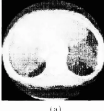
We have tested the proposed near-closed-form method on three image sequences. One of these sequences is generated from a real CT image (shown in Fig. 1(a)). The other two sequences, namely the Text-i and Text-2 Sequences (Fig. 2), are generated from a synthetic image (shown in Fig. 1(b)). The subsequent 19 framesofall three sequences aregeneratedby introducing random subpixel displacements to the first frames, i.e., the reference frames, shown in Figs. 1(a) and (b).

The CT Sequence does not contain any intensity variations. On the other hand, we have simulated both contrast and brightness variations on the Text-i Sequence, and only contrast variations on the Text-2 Sequence. In order to introduce the intensity variations to the subsequent frames of Text-i sequence, the pixel intensities in the frames are first multiplied by y, and ijisadded afterwards as explained in (13). If we let k denote the frame number, the values

of and ij

chosenfor the kt frame are defined in our experiments as

7(k) =

1+70k (27)

r(k) =

ijok (28)

For the Text-i Sequence, we have set 7(k) =1—_O.02(k—₁₎and ij(k) =_—2(k—

i),

whereas for the Text-2 Sequence,

we have set 7(k) = 1—_O.04(k—₁₎

and i(k) =

0. In addition to intensity variations, a 10 dB white Gaussian noise is

added to each frame in the Text-i and Text-2 Sequences to simulate any observation noise. A 5 >< 5 uniform blur is applied to each frame prior to subpixel displacement estimation to reduce the effects of bilinear interpolation and

of any additive noise. The simulations are carried on a block of size approximately 100 x iOO pixels, that contains sufficient intensity variations.

In Fig. 3, we compare the performance of the proposed near-closed-form solution to that of the spatio-temporal differentiation method, phase and cross correlation surface interpolation methods and the exhaustive search method (the accuracy of the exhaustive search method is chosen to be pixels) . We observe that the cross correlation method performs nearly as well as the proposed near-closed-form solution for the Text-i and Text-2 Sequences. However, the performance of the cross correlation method degrades significantly for the CT Sequence. On the other hand, the performance of the differentiation method is close to that of the proposed near-closed-form solution for the CT and the Text-i Sequences, while it degrades considerably for the Text-2 Sequence. We conclude from Fig. 3 that the proposed near-closed-form solution consistently gives the best results for all the sequences considered.

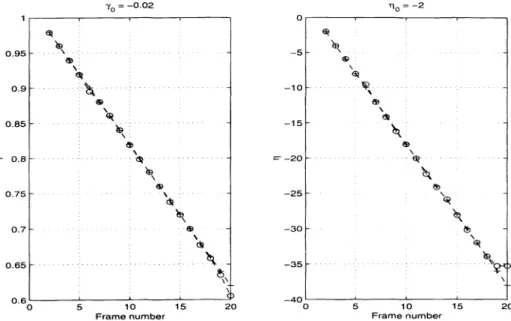
In Fig. 4, the plots of y(k) and ij(k) versus the frame number (k) are given for the Text-i Sequence. It can be seen that the near-closed-form solution is able to estimate the parameters 7(k) and i1(k) for each frame (k) almost perfectly.

The CPU times for all of the methods compared in Fig. 3 are nearly the same, except for the exhaustive search method, which is significantly slower than the others.

We have also carried out experiments to test the performance of the proposed affine motion estimation algorithm on the CT image shown in Figure 1(a). The transformed image is the counter-clockwise rotated version of this reference image by iO degrees. The sizes of the three blocks are chosen as 79 x 79. The correct affine motion parameters between the rotated and reference images are given by

0.9848 —0.1736 0

T* 0.1736

0.9848 0

. ₍₂₉₎

—40.4787 48.2391 1

The affine parameter estimation algorithm is executed five times and the overall affine motion matrix Tk obtained after iteration k is:

0.9790 —0.i75i 0

0.9852 —0.1704 0 0.9858 —0.1738 0 T1

=

0.1926 i.0i24 0 ,T2 = 0.1779 0.9825 0 ,T3 = 0.1730 0.9836 0 , (30) —39.2509

43.6864 i

—40.399i 47.3248 1

—39.699 48.3858 1

0.9849 —0.1738 0 0.98497 —0.1737 0 T4 0.1732

0.9849 0

_,T5

=

0.1734 0.9850 0 —39.4366

48.1345 1

—39.4734 48.0752 1

It can be seen from the above matrices that, as the iteration number k increases, the matrix Tkbecomes a closer

estimateof the correct matrix T*. The incremental matrices Ak'safter the kthl iteration are:

i.0036 —0.0004 0

0.9997 —0.0032 0

A2

=

—0.0i52

0.9706 0

A3

=

—0.0049 1.0017 0 (31)

0"

TEXT

Hglll'( 1. a) I lie first train' of the (1 4i'quolice. (h) the Inst Iranie of tii' I'xt I anti I'Nt—2

H'1iieiii'i's

Figiir'

2. (a) 'I'he last frameof'the Iext—l (1110000. (h) 'liii' last t'raita' of I Iii' 'Ii'xt—2

_'iit'tiei'.

Figure 3.

'tIn'

niagnit 11(10of thit- _displacement estmiat loll errorvector

( (i1 ), ((I')).

().I))1I2 P.H(1P2 I) I J)U() I P.1)111)!

14 0,11110:1 1.uuld 1)

,.

1—, 0.110112 1(11)1)1

1)21 hi) —11.305)) 1 —Oft-lIP

-)1.ftT

iti' that /c

.l4t_ ,..;l',]. A > 2. It (all to' ol)served that titi' off-diagonal laratI't)'r it the iicretiieutat

ileitrIi' .). llliimiotonicaiiy get siiialler after each iteration and hence

_{:.;1fpirii;Ii'ln}

ti tIi iil'tititv nat rix. 'this

that. lie proios'd algorithmconverges to the correct alliiii' 01)110(1 iaOIIIl)li'I'

045 r

0 4

Sinhpixel Displacement Estimation Errors

A Closed—terre S iilnntii,r'

E

e Spatio—tenrporal ctitferenialnciri

C Exhaustive search

D Cross—cn,rrelation interpolation E Phase-- correlation intorpolat Kr]

E

1_002

1 C, . 0.95 ' •

:

. _—5. . \ _. 0.9 • • • . . . _—10 . _.

,

065 5

101520

Framenumber Frame number

Figure4. The y and r values found for the Text-i Sequence in which (yo , io)

=

(—0.02,—2). The "o" and "+" signsdenote the estimated and true values for '(onthe left) and ij (on the right), respectively.

7. CONCLUSION

In this paper, we introduced a novel near-closed-form solution for subpixel accuracy stabilization of unsteady image sequences. In the proposed method, the mean-squared error over subpixel displaced frames is minimized with respect to the motion vector components analytically. The method is made robust to intensity variations between frames by modeling such variations using contrast and brightness parameters. If a closed-form solution can not be found, which happened rarely in our experiments, an efficient exhaustive search method is used. The performance of the proposed near-closed-form solution is compared with the spatio-temporal differentiation method, phase and cross correlation surface interpolation methods and the exhaustive search method. It is shown that the near-closed-form solution outperforms the other methods in terms of motion vector estimation errors. Finally, the proposed near-closed-form solution is utilized for estimation of affine motion parameters between two frames, using three point correspondences.

APPENDIX A. BASIC SUMMATIONS

In the following, the summations are over ni, n2 E B and the results of the summations are normalized by N1N2. Thus, for example,

:

si(ni,n2)

=

_N1N2

i:

si(n1,n2).

fljfl2 E L3

Thedefinition of the basic summations are now given as follows. A0,0 =

_Sl(fl1,fl2),

A00; 0,0

S(fll,fl2),

Bo,o; i,,

= Sl(nl,n2)s2(n1

+i,n2 +j),

z,j

=

—1,0,1,

D,3 = S2(fl1

+2,fl2 +j),

= 101

Di,3; k,

=

32(fll + Z,Th2 + j)s2(ni + k,n2 + £),

k, =

—1,0,1, (z,

k) (j,

e) (±1,+1).

APPENDIX B. MSE COEFFICIENTS

Inthe_{following, we express} . . , interms of the basic summations. The scalars I and J are determined by the quadrant number as defined in Equation (6).

= Ao,o;_{0,0 2B0,o;0,0}

+

_{Do,o; 0,0,}

= 21(Bo,o;0,0 Bo,o; 1,0 — Do,o; 0,0 Do,o;

i,o)

= 2J(Bo,o;0,0 Bo,o; o,j —Do,o; o,o + Do,o; o,)

= 21J(_Bo,o; _{0,0 + Bo,o; 1,0 + Bo,o; o,j Bo,o; i,j}

+2D0,o; 0,0 2Do,o; 1,0 —2Do,c);0,J + Do,o; i,j + Di,o; o,j),

= Do,o;_{0,0 2D0,o; 1,0 + Di,o; 1,0,}

Do,o;0,0 2D0,o; 0,J + D0,j; 0,J,

(]i)

= 2J(_Do,o;_{0,0 + 2Do,o; 1,0 + Do,o; o,j —}Do,o;i,j —Di,o; 1,0 —_Di,o;

_{o.j + Dj,o j,j),}

= 21(_Do,o; 0,0 + Do,o; 1,0 + 2Do,o; o,j —Do,o;i,j —Dj,0;o,j —_Do,j;

_{o,i + Do,j; i,j),}

C Do,o; 0,0

2D0,o; 1,0 —2Do,o; o,j 2D0,o; I,J + Di,o; 1,0 + 2Di,o; o,j

2Dj,o; i,j + Do,j; o,j —2D0,j;

i,j + Dj,j; j,j.

APPENDIX C. THE COEFFICIENTS OF THE FIFTH ORDER POLYNOMIAL

Ill the following, we give the expressions for .

. . , E

in terms of ._{. . ,} For notational simplicity, we

omit the superscript (')inthe following equations as the expressions are the same for each i =1,2, 3, 4.

E0 =

_-4C2C

+ 2C1C3C4 -CC€ E1 =

_-8CC5

+ 4C1C4C7 + 2CC4 -8C2C4C6

-

2C?G5

=

2C1C6 C7 -4C2C+ CC6 -8C2C4C8

-

16C4C5C6

-

2C1C3C8 + 6C3C4C7

=

_-8C2C6C8+ 4C4C - 16C4C5C8+ 4C3C6C7 -_8C5C

=

_3C6C

—

_4C2C

—

_{16C5C6C8 2C3C7C8} r' _—

c2c oc ç-2

-7'--'8— 0L5L8

APPENDIX

D. THE COEFFICIENTS FOR CONTRAST AND BRIGHTNESS

PARAMETERS

Let

1

Then

=

_[Bo,o;

0,0 —_Ao,0D0,o]

=

_I[Bo,o;

_{i, Bo,o; 0,0}

_Ao,o(Di,o—

Do,0)]

=

_J[Bo,o;

_{o,j Bo,o; 0,0 —Ao,0(D0,j}

—

Do,o)]

=

_IJ[Bo,o;

_{0,0 Bo,o; 1,0}

_{Bo,o; ,j}

_{+ Bo,o;}

_i,j

_Ao,o(Do,o—

D1,0—

D0,

+ Di,j)]

and

=_L{Ao,o;0,0D0,0 —_{A0,0Bo,o;o,o]}

rI

r'IU

+

f'I

'r'og

— fO

fOj

+

f'1c[H

—

r'f

0'Ic[

_

r'o o'I

o'Ia

+

O'IQ7j

+

I-'I

o'oa

+

ro

o'I

o'oa

_

o'o O'OGH_

r'I

o'oU:D

_

r'o

'o'oUD

+

o'I o'o O'O9D

_

o'o 'o'oVD

+

OOvg

+

H

(z)D [

rIa?H

O'IU?H +

fl

f'OQ

+

UI r'o

r'o

— r'oa(CH —

H)

+

0'1 O'O r'o

o'oj

+

o'o o'oU(H

_

H)

— o'ogz — o'I ['0 o'oU(CD —

D)

+

°'° o'oG.(cO

_

o'o 0'0VcDD

+

o'ov(cDH +

DH)

+

HH]Z

(t)3 {

rIQIH

— r'OUtH

+

o'IG

+

r'o o'I

°"a

— o'IU(CH — tH)

+

''

'o'oG-_ f'o o'oU

+

o'I

o'oU

+

o'o o'oU(H

_

IH) —

ri

o'oUtD r'o 'o'OG-TD+ 0'I o'oU(D

_

'o)

+ °° o'oU(D

_

tDH)

+

oov(D1H

+

o'oV:DID o'o

+

JJtH]

= (z)O r'o r'oq

+

1'°UH

— 0'0U

_

oo

o'o

ro

o'ogD

o'oo'o-D

+ o'o o'oVD

+

O'OVDH +

H

()D oI 0'1a

+

°"Q'HZi —

'I

O'O

— O'O O'O O'OQtH+ 0'I

o'ogTg

_

O'OO'O9t9 0'0VD

+

OOVtDtH +

H

=

()G [rIuoH roU(IH

-

OH)

+

'°

oIU

+

o'IU(zH

-

OH)+

r'I

'o'oU

+

r'o

'0'0a

— o'oG- _ o'o

o'oq

+

o'oU(oH

H

—

H

+

tH)+

r'I

o'oUoD

_

['0 o'og(

t

_

0'I ooU(D

_

OD)

+

o'o(oD CD

_

D

+

tD)+ o'o o'ov(DoD +

+

o'oy(ODCH

+

£DOH

+

tDH

+

DtH) +

H°H

+

HtH]

=

()O [ r'OQO]J

_

r'o o'oj- + o'o

o'o

—

o'o(pj

— ['0 ooUoD o'o

OO(rj

_

D)

+ °° '0'0VD0D +

oo(ojj

+

D°H)

+

o]g

(z)D { O'IQOH o'I O'OG + o'o o'oa — O'OG(tH OH)+ 0'I

0'009

— o'o — 09)

+

'°

°'°V'D°D +

oo(o9tjq

+ 190H) + IH0HJ

=

(i)O °'° °°G

+

°°U°H

—

00 008

09

— 00 OOyO9

+

0'OVO9OH

+

°H

=

()D .()

uoinb

UI

pupp

si

qwnu

uiipnb

cq

pu

uap

ii

_'uiMOITOJ

M

_AT

_suoissjdx

oj

(i)O UT

SUhi

JO

iusq

suoiuimns

qji,

s.I%Ies

i

pii

r

uj

SNOLLVDIVA

ALISNaLNI

JO

SvD

JLL

NI

SLNIDIJJOD

aSJ,

E

XIQNEEddV

(9)

uoinb

UT

U&I

S

Z

qmnu

uipnb

q

puimJp

UT

f

pU

'"01

U

[(ri

o'og

+

00

— 01 008 — 00 0'Og) O'Ov_

('u

+

r'OU —

°"a

— o'oa)O'O

00v]vfI

=

(2)H [(o'o

'o'o

ro

'008) o'ov — (o'oU — r'oG)o'o 'o'ov]v[

=

(2)H

APPENDIX F. THE COEFFICIENTS FOR THE BRIGHTNESS PARAMETER

=

_D0,0

-

_A0,0

=

_I(D1,0— Do,o)

=

_J(D0,

— Do,0)

=

_IJ(D0,0—• D1,0—D0,j

+ Di,j)

In the above, the scalars I and J are again determined by the quadrant number i as given in Chapter 2.

APPENDIX G. THE COEFFICIENTS FOR THE CONTRAST PARAMETER

=

_{Bo,o; o,o/Ao,o; o,o}

=

_{I(Bo,o;1,0 Bo,o; o,o)/Ao,o; 0,0}

=

_{J(Bo,o; 0,J Bo,o; 0,0 )/Ao,o; 0,0}

=

_{IJ(Bo,o;0,0 Bo,o; 1,0 —Bo,o; o,j + Bo,o; j,j)/Ao,o; o,o}

In the above, the scalars I and J are again determined by the quadrant number i as given in equation (6).

REFERENCES

1. L. C. Brown, "A survey of image registration techniques," ACM Compnting Surveys 24, pp. 325—376, 1992. 2. C. D. Kuglin and D. C. Hines, "The phase correlation image alignment method," Proc. IEEE InLConf.

Cyber-netics Sociely ,pp. 163—165, 1975.

3. Q.Tian_{and M. N. Huhns, "Algorithms for subpixel registration," Computer Vision, Graphics, and Image}

Pro-cessi'ng 35, pp. 220—233, 1986.

4. A. M. Tekaip, Digital Video Processing, Prentice-Hall, New Jersey, 1995.

5. S. D. Conte and C. D. Boor, Elementary Numerical Analysis—An Algorithmic Approach, McGraw-Hill, New York, 1980.

6. ç.

Eroglu,"Subpixel accuracy image registration with application to unsteadiness correction," Master's thesis, Bilkent University, 1997.

7. C. S. Fuh and P. Maragos, "Affine models for image matching and motion detection," Proc. IEEE ml. Conf.

AcousL. Speech, Signal Process. ,pp. 2409—2412, 1991.