The financial analysis of postmerger performance of surviving firms

(1)

THE FINANCIAL ANALYSIS OF POSTMERGER PERFORMANCE OF SURVIVING FIRMS

Alövsat Müslümov*

ABSTRACT

This paper examines the synergy created in the merger process, its sources and factors that influence its magnitude using a sample of 56 mergers from U.S. industries completed within 1992-1997. Research findings indicate that mergers are resulting in the synergy gains, which is measured by operating cash flows relative to the industries. The cash flow increases do not come from gaining monopoly position and cutting capital investments and labor cost. The cash flow improvements come from the more productive usage of assets in generating sales. The subsample studies show that cash flow improvements are particularly strong in high overlap, equity-financed, value and larger merger subsamples.

*_{Ph.D. in Finance, Assistant Professor, Faculty of Economics and Administrative Sciences, Doğuş University,}

Istanbul, Turkey. The paper is based on one of the parts of my Ph.D. dissertation, entitled “The Financial Analysis of Mergers” (Boğaziçi University, February 2001). I would like to thank to Prof. Dr. Özer Ertuna, Prof.Dr. Cudi Tuncer Gürsoy and an anonymous referee for their many insightful comments and helpful suggestions. The financial support of Selcuk Altun in purchasing the Compustat Database and Ali Polat in

(2)

I. INTRODUCTION

Financial literature suggests that merger decision may be the result of one or more of the following motives: synergy, agency, and hubris. The synergy motive implies that merging firms expect synergetic gains that result by merging the resources of the two firms. The gains may arise from various sources, such as: potential reductions in production or distribution costs, realization of economies of scale, vertical integration, adoption of more efficient production or organizational technology, increased market power in product markets, increased utilization of the acquirer’s management team, reduction of agency costs by bringing organization-specific assets under common ownership, elimination of inefficient target management, the use of underutilized tax shields, avoidance of bankruptcy costs, increased leverage, other types of tax advantages. Synergy motive predicts that the combined firm generates cash flows with a present value in excess of the sum of the market values of the bidding and target firms.

The agency motive, which is based on the agency theory, suggests that takeover occurs since managerial motives dominate takeover market and acquirer’s management enhances its welfare at the expense of acquirer shareholders. Jensen (1986) suggests that managers may undertake acquisitions simply to increase the sizes of their firms, since managerial compensation and power often increase with the level of sources under a manager’s control. Shleifer and Vyshny (1989) however, suggest that managers may undertake acquisitions of firms for which they would be the best possible managers for the purpose of enabling them to attract higher compensation from their shareholders and increase their job security. They suggest that management might acquire firms that enhance the dependence of the firm on their own skills even though such announcement acquisitions might reduce the value of the firm. Harris (1994) suggest that although a firm’s shareholders are likely to be better off if their firm is the target rather than the acquirer, the firm’s manager, may be better off if his firm is the acquirer, since the target’s manager usually losses his job following a takeover, whereas the acquirer’s manager usually retains his. According to Harris’s model, a manager’s fear that the firm with which his firm can create synergy gains will take over his firm, if his firm does not take it over, makes him want his firm to be acquirer.

The hubris hypothesis suggests that managers make mistakes in evaluating target firms, and engage in acquisitions even when there is no synergy (Roll, 1985). It is most likely because acquirer companies overestimate their abilities to manage an acquisition. The hubris hypothesis relies on the perfect form of market efficiency. In the case of strong-form efficient markets no gains from the takeover could be observed, since these takeovers do not bring any operational or financial synergy and doesn’t bring a solution to agency problems (since there is not any agency problem).

Financial literature provides evidence that merged firms show significant improvements in postmerger cash flows. Healy, Palepu and Ruback (1992) examine the post-acquisition operating performance of merged firms using a sample of the 50 largest mergers between U.S. public industrial firms completed in the period 1979 to mid-1984. They have found significant improvements in operating cash flow returns after the merger, resulting from increase in asset productivity relative to their industries.

The primary objective of this paper is to study the magnitude of the synergy created in the merger process and specify successful merger types. For this purpose, we collected a sample

(3)

of 56 mergers between U.S. public industrial firms completed between 1992 and 1997. We establish two-staged variable analysis model. In the first stage, we measure where there is synergy postmerger. We used experimental design to measure postmerger performance improvements of surviving firms, following Healy, Palepu, and Ruback (1992). Our cash flow measures are industry-adjusted and unaffected by the method of payment and the method of accounting of transaction.

The present study provides validity check of the study of Healy, Palepu and Ruback (1992) in a unique time setting. Our merger sample that covers 1992-1998 period is unique and has not been analyzed in the previous researches in empirical literature. This period is characterized as a heavy merger wave period in U.S. industries. The U.S. industries were forced to restructure themselves in these years due to technological developments, growing competition, and pressure from demand side. The merger patterns and anticipated gains varied considerably across industries.

Media, telecommunications and computer industries were involved in heavy takeover activities as a result of swiftly evolving digital technology, which was driving these industries together. The primarily two technological advances; digitization and fiber optics, were converging these industries on the “information superway”. The distinctions between telephones, televisions and computers were starting to blur as a result of digital technologies. The broken monopoly of telecommunications firms in the USA, pushed firms to merge in order to be competitive and to offer customers every sort of telephony: local, long-distance, and Internet access. Geographical market expansion desires were another motivation of mergers in these industries.

The computer industry was trying to challenge the growing power of Microsoft in the software market, by merger and joint ventures. A wave of intelligent, handheld devices, running non-Microsoft software attracted almost all of the computer companies and pushed them to takeovers. The defense industry was trying to restructure itself in the face of Pentagon’s intention to reduce the budget allocated to defense expenditures, which would result in smaller number of integrated suppliers. The pharmaceutical industry was going to be vertically integrated. The drug companies were merging with pharmacy benefit management companies, middlemen with massive buying power that provide prescription drugs for their insured customers at knockdown prices.

Our research findings favor synergy theory of the mergers. It is found that merged firms show significant improvements in operating cash flows relative to their industries postmerger, resulting from increases in asset productivity relative to their industries. Postmerger cash flow improvements do not come at the expense of the long-term performance and do not reflect wealth transfer from other stakeholders to shareholders. This result suggests that postmerger cash flow improvements can be attributed to the synergy resulting from merger.

The subsample analyses show that high overlap, equity-financed mergers experience significantly higher cash flows whereas low overlap and mixed-financed mergers fails to perform better after merger. In the other hand, it is found that bidders with high price-to-book ratios are motivated by hubris. Their mergers fail to create additional value, whereas bidders with low price-to-book ratios are more prudent in their merger decisions. The combined size of bidder and targets are found to be effective on the postmerger performance of the mergers. Significant improvements in cash flows are observed in bigger mergers, whereas smaller mergers do not experience significant cash flow improvements after merger.

(4)

The remainder of the paper is organized as follows. Section II describes sample and data used in the study. Section III describes the research methodology. Section IV analyzes postmerger performance of merged firms. Section V discusses previous empirical research and compares the research findings. Section VI gives a brief conclusion.

II. SAMPLE AND DATA

We collected a sample of mergers between 1992 and 1997. The source of the merger data is Mergerstat. The primary database consists of 629 merger bids meeting the below-mentioned restrictions;

1. There is a merger offer to purchase stock in the company. 2. The details of the offer appear in Mergerstat.

3. Transaction date lies between 1992 and 1997.

4. Transactions valued at less than $ 350 million were eliminated. Banks, insurance, and railroad companies were eliminated, since they are subject to different regulations. 5. Country of bidders and targets is the USA. Acquisitions by foreign concerns were

eliminated.

6. The deals that did not obtain complete ownership of the target were eliminated. 7. The mergers that were later cancelled were eliminated.

From this primary database we select our sample according to the following criteria:

8. The acquiring company is required to have at least, three years premerger and two years postmerger financial and market data available on the Compustat tapes, whereas the requirement for the target company is three years premerger financial and market data.

9. The size of target should exceed 5% of the size of acquirer. Target firm size is computed from Compustat as the market value of common stock plus the net debt and preferred stock at the beginning of the year before the acquisition.

10. Some companies are involved in more than one merger bid. The merger cases involving these bidder firms are eliminated from the analysis, since there are distorting effects of crossing merger cases.

These selection criteria reduce our initial sample of 629 merger cases to 56. This sample size is satisfactory for the analysis purposes. Healy, Palepu, and Ruback (1992) conducted the postmerger performance analysis with 50 cases, whereas this number was 38 in Clark, and Ofek (1994).

Summary statistics for aggregate, average, and median deal size and total number of mergers according to calendar years are reported in Table 1. The last two years capture more than half of the total number and aggregate dollar value of mergers. Average deal size is 2,983 million dollars, whereas median deal size is 1,169 million dollars. The average and median deal sizes suggest that the study is focused on larger mergers.

(5)

Table 1

Summary statistics for aggregate, average, and median deal size and total number of mergers according to calendar years in 56 merger cases over the period 1992-1997.

Year Total

Number of Mergers Aggregate Deal Size (Million Dollars) Average Deal Size (Million Dollars) Median Deal Size (Million Dollars)

1992 3 1,222 407 406 1993 6 14,213 2,369 1,154 1994 5 4,410 882 828 1995 13 46,607 3,585 1,440 1996 15 83,735 5,582 2,184 1997 14 16,872 1,205 772 Total 56 167,059 2,983 1,169

The source of the financial and market data is Compustat (North American). III. RESEARCH METHODOLOGY

3.1. Testable Predictions

Since our primary objective is to test whether there are any performance improvements after the merger, we examine the cash flow, profitability, operating efficiency, output, and capital investment variables. Specifically, we test the hypotheses that mergers (1) increase the surviving firm’s cash flow, (2) increase the surviving firm’s cash flow margin, (3) increase surviving firm’s asset productivity, (4) increase surviving firm’s operational efficiency, (5) increase surviving firm’s capital spending, (6) decrease surviving firm’s employment cost. Table 2 presents our testable predictions and the empirical proxies we employ. The testable predictions are held in the similar line with the study of Healy, Palepu, and Ruback (1992) in order to provide comparable results.

Table 2

Summary of Testable Predictions

This table details the economic characteristics we examine for changes resulting from mergers. We also present and define the empirical proxies we employ in our analyses. The index symbols POST and PRE in the predicted relationship column stand for postmerger and premerger, respectively.

Variable Proxies Predicted Relationships

Return on Assets (ROA) = EBITD /Total Assets ROApost>ROApre

Cash Flow

Return on Equity (ROE) = EBITD /Total Equity ROEpost>ROEpre

Asset Turnover (AT) = Sales/Total Assets ATpost>ATpre

Cash Flow

Components Return on Sales (ROS) = EBITD /Sales ROSpost>ROSpre

Sales Efficiency (SALEFF) = Sales/Total Employment SALEFFpost>SALEFFpre

Operating

Efficiency EBITD Efficiency (NIEFF) = EBITD/Total Employment NIEFFpost>NIEFFpre

Capital Expenditure to Sales (CESA) = Capital

Expenditure/Sales CESApost>CESApre Capital

investment

Capital Expenditure to Total Assets (CETA) = Capital

Expenditure/Total Assets CETApost>CETApre Employment Pension Expense Per Employee (PEE) = Pension PEEpost<PEEpre

(6)

3.2. Variables

We use two different cash flow variables to measure improvements in operating performance. We use EBITD deflated by the market value of assets (market value of equity plus book value of net debt), and total equity (market value of equity) to provide a return metric that is comparable across firms.

The market value of assets, measured at the beginning of the year, is the market value of equity plus the book values of net debt and preferred stock. We define EBITD, measured over the year, as sales, minus cost of goods sold and selling and administrative expenses, plus depreciation and goodwill expenses. This measure excludes the effect of depreciation, goodwill, interest expense and income, and taxes. It is therefore unaffected by the method of accounting for the merger (purchase or pooling accounting) and the method of financing (cash, mixed or equity). As discussed in Healy, Palepu, and Ruback (1992) these factors make it difficult to compare traditional accounting returns of the merged firm over time and cross-sectionally.

We exclude the change in equity values of the target and acquiring firms at the merger announcement from the asset base in the postmerger years. For the target and acquirer, the change in equity values is measured on the beginning of the month before the bid offer is announced to the date the target is deleted from Compustat, which is regarded as the delisting date from trading on public exchanges. In an efficient stock market these revaluations represent the capitalized value of any expected postmerger performance improvements. If merger announcement equity revaluations are included in the asset base, measured cash flow returns will not show any abnormal increase, even though the merger results in increase in operating cash flows.

If there are improvements in cash flow returns in the postmerger period, it can arise from a variety of sources. These include improvements in cash flow margins and greater asset productivity. Cash flow margin, which is EBITD on sales, measures the pretax operating cash flows generated per sales dollar. Asset turnover measures the sales dollars generated from each dollar of investment in assets (market value of the assets). The variables are defined so that their product equals to the EBITD on total assets, first cash flow variable.

Operating efficiency variables primarily deal with the increased usage of labor to produce more output. Sales and EBITD on total employment provide a measure to test the improvements in operating efficiency.

Improvements in cash flows may be achieved by focusing on short-term performance improvements at the expense of the long-liability of the firm. To assess whether the merged firms focus on short-term performance improvements at the expense of long-term investments, we examine their capital investments. Two empirical proxies are employed to measure capital investments; capital expenditures to sales and capital expenditures to total assets (market value of the assets).

Mergers give the acquirer an opportunity to renegotiate explicit and implicit contracts to lower labor costs and achieve a more efficient mix of capital and labor. Because we are unable to obtain sufficient data on wages directly, we examine pension expense per employee to analyze changes in labor costs in years surrounding the mergers. However, the caution

(7)

should be made in the interpretation of this variable, since this variable suffers from identification problem. Firms may not be as flexible in their pension expenses as they would be in their direct compensation contracts.

3.3 Performance Benchmark

We aggregate performance data of the target and bidding firms before the merger to obtain the premerger performance of the combined firms. In the calculation of variables for premerger years total assets, sales, EBITD, capital expenditures, pension expenses, and number of employees are taken as the sum of the values for the target and acquiring firms. The variable values of surviving firm are used in the postmerger years.

Comparing the postmerger performance with this premerger benchmark provides a measure of the change in the performance. But economic factors have much effect on the postmerger performance of the merged firms and some of the difference between the premerger and postmerger performance could be due to economywide and industry factors, prior to a continuation of firm-specific performance before the merger. Hence, we use industry-adjusted performance of the target and bidding firms as our primary benchmark to evaluate postmerger performance.

Industry-adjusted performance is calculated by subtracting the industry median from the sample firm value for each year and firm. we use Compustat SIC industry definitions, and exclude the target and acquiring firms’ values from the industry median value computations. Industry values for the sample firms are constructed by weighing median performance measures for the target and acquiring firms’ industries by the relative asset sizes of bidder and target at the beginning year of the merger announcement.

At last, but not least, a caution should be made on the synergy assumption utilized in the present study. The synergy assumption of the current study is that if the synergy effect is present, the total cash flows of merged firms will be greater than the simple sum of cash flows of the parts that is bidder and target firms. Research findings should be interpreted within this window, since if the synergy assumption is incorrect, then the pre-merger period would be misrepresented by the mere summation of the two firms.

3.4. Research Methodology

To test the research predictions, we first compute empirical proxies for every company for a seven-year period: three years before through three years after mergers. we then calculate the median of each variable for each firm over pre- and postmerger windows (premerger= years – 3 to –1; postmerger = years +1 to +3). Year 0, the year of the merger, is excluded from the analysis since the variable values for this year are not comparable across firms and for industry comparisons.

Having computed industry-adjusted pre- and postmerger medians, we use the nonparametric Wilcoxon signed-rank test as our principal method of testing for significant changes in the variables following Megginson, Nash and Van Randenborgh (1994). The financial ratios do not follow normal distribution, making it difficult to interpret the findings of the parametric

(8)

analysis. The small sample sizes in subsample analyses, also, lead to the selection of nonparametric tests as a suitable method of testing postmerger performance improvements. We base our conclusions on the standardized test statistic Z, which for samples of at least 10 follows approximately a standard normal distribution. In addition to the Wilcoxon test, we use a (binomial) proportion test to determine whether the proportion (p) of firms experiencing changes in a given direction is greater than would be expected by chance (typically testing whether p = 0.5). Given the wide variance in firms, and industries, finding that an overwhelming proportion of firms changed performance in the same direction may be at least as informative as a finding concerning the median change in performance.

3.5. Subsample Analysis

In addition to analyzing the full sample of merged companies, we perform similar tests for below mentioned subsamples. The percentage distribution of the subsamples is provided in Table 3.

Table 3

Distribution of Subsamples

This table details the absolute and percentage distribution of subsamples defined in the body part of the text. Total 56 merger cases present in the total sample of this study.

Variable Number Percentage

Business Overlap Subsets

High Overlap 33 59 %

Medium Overlap 4 7 %

Low Overlap 19 34 %

Method of Payment Subsets

Cash 12 21 % Mixed 11 20 % Equity 33 59 % Value-Growth Subsets Value 17 30 % Growth 39 70 %

Combined Size Subsets

Small 28 50 %

Big 28 50 %

1. Business Overlap Subsamples: Theoretical financial literature suggests that strategy is an important determinant of the improvements in the postmerger performance, therefore, it is reasonable to hypothesize that mergers by firms that have overlapping businesses will show greater cash flow improvements than mergers between firms with no overlap. we examine this proposition by classifying our sample mergers as those with high, medium, and low business overlap between the target and acquiring firms. High overlap mergers are merger cases between those bidder and target firms whose at least three first SIC Code numbers are the same, whereas in medium overlap mergers the first two SIC Code numbers similar. The remaining mergers are classified as low overlap mergers. Sample analysis show that 33 (59%) out of 56 mergers are

(9)

high overlap mergers, whereas 4 (7%) cases are medium overlap and 19 (34%) cases are low overlap mergers.

2. Method of Payment Subsamples: The method of payment of financing is frequently cited as important to the ultimate success of mergers. The effect of method of payment is analyzed by dividing total sample to three subsets based on the form of payment. The first subset is called equity-financed and includes cases where only the acquirer’s common stock was used to pay for an acquisition. The second subset is called cash-financed and includes cases where only cash was used for payment. The third subset is called mixed-financed and includes all other cases in which the payment terms were neither pure stock nor pure cash. In some cases, both stock and cash were used and in other cases cash and senior securities were used. Sample analysis show that 33 (59%) out of 56 mergers are equity-financed mergers, whereas 12 (21%) cases are cash-financed and 11 (20%) cases are mixed-cash-financed.

3. Value-Growth Subsamples: Theoretical financial literature suggest that companies with high price to book ratios (‘growth’ firms) are more likely to overestimate their own abilities to manage an acquisition and motivated by hubris (Rau and Vermaelen (1995)). Therefore, the takeovers by growth firms destroy shareholder value. On the other hand, companies with low price to book ratios (‘value’ firms) are more prudent before approving acquisitions. Since these acquisitions are not motivated by hubris, they should create shareholder value. we rank the mergers into separate subsamples based on bidders’ price to book ratio relative to their industries’ price to book ratio at the beginning of the year of merger announcement. Bidder companies’ price to book ratio is compared to the industry’s median price to book ratio in the beginning of the year prior to announcement. If bidder companies’ price to book ratio is higher than industry’s median price to book ratio book, the merger case is classified as ‘growth’ merger, otherwise as “value” merger. As a result of this ranking, 17 (30%) mergers appeared to be ‘value’ mergers and 39 (70%) bidders as ‘growth’ mergers.

4. Combined Size Subsamples: we also examine whether the combined size of bidder and target influences postmerger performance of the surviving firm, we divide total sample to two different subsets according to combined size of the bidder and targets. Combined size is calculated as the sum of bidder and target firm sizes in the beginning of the year prior to announcement. Total assets are calculated by summing market value of equity and book value of total debt and preferred stock. we classify mergers as “larger” and “smaller” according to their size relative to the median for all firms in the sample. If the combined size of merger is greater than or equal to the calculated median of the sample, the merger case is classified as a larger merger, otherwise as a smaller merger. Since merger cases are ranked relative to their median, both subsets have an equal number (28 mergers) of merger cases.

IV. Empirical Results

In this section we present and discuss our empirical results for the full sample of mergers, and for the four subsamples. we first present and discuss our empirical results (in Table 3 and Table 4) for the complete sample of 56 mergers. Then we discuss our results for the following subsamples of our data: high overlap versus medium overlap versus low overlap mergers

(10)

(Table 51); cash financed versus mixed financed versus equity-financed mergers (Table 6); value versus growth mergers (Table 7); larger versus smaller mergers (Table 8). For each of these partitions, we examine and report (in the text and in Tables 5 to 8) whether each subsample of firms experience significant changes in the variable values after merger. We also test whether the difference between the value changes for the subsamples are significant.

Cash Flow Changes

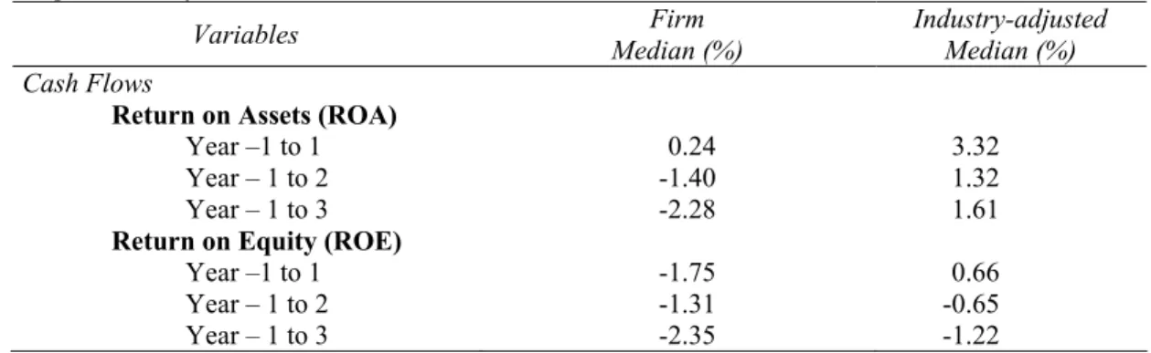
Table 3 reports the changes in cash flows in years 1 to 3 relative to the year before merger. Firms’ median ROA increase by 0.24% in year 1, decrease by 1.40% in year 2, decrease by 2.28% in year 3 relative to year -1. It seems that there is downward trend in firm’s cash flows in the postmerger period. However, the sample firms’ industries experience decline in cash flows also, and this decline is greater than sample firms’. Therefore, industry-adjusted cash flows increase by 3.32% in year 1, 1.32% in year 2, and 1.61% in year 3 relative to year -1. Apparently, merger-related cash flow improvements are immediately observed following the merger.

Table 3

Median change of variables in postmerger years relative to the year before the merger

This table presents median change of variables in years 1 to 3 relative to the year before the merger (year -1). Year –1 value for the combined firms is weighted averages of target and acquirer values, with the weights being the relative asset values of the two firms. Postmerger values use data for the surviving firms. Industry-adjusted variables are computed for each firm and year as the difference between the sample firms’ growth rates in that year and growth rates for variables in the same industry. Target and acquirer industry values are weighted by the relative size of the acquirer and target firms in year –1.

Variables _{Median (%)}Firm Industry-adjusted _{Median (%)} Cash Flows

Return on Assets (ROA)

Year –1 to 1 0.24 3.32

Year – 1 to 2 -1.40 1.32

Year – 1 to 3 -2.28 1.61

Return on Equity (ROE)

Year –1 to 1 -1.75 0.66

Year – 1 to 2 -1.31 -0.65

Year – 1 to 3 -2.35 -1.22

Another cash flow proxy, ROE, however, shows below-industry performance comparing to year –1. Industry-adjusted ROE increases by 0.66 % in year 1, and then decreases by 0.65% in year 2, and 1.22% in year 3 relative to year -1.

Table 4 reports that in accordance with research predictions, industry-adjusted ROA increases significantly after merger. The industry-adjusted mean (median) increase in ROA after merger is 1 percentage points (1 percent) and 61 percent of all firms experience increasing ROA after merger. These test statistics are all significant at the 10 percent level2. This result suggests that mergers create synergy. Cash flows deflated on the market value of stocks (ROE) do not show significant changes after merger.

1_{Table5 through Table 8 are provided in the appendixe.}

(11)

Table 4

Postmerger Performance Analysis: Summary of Results from Tests of Predictions for the Full Sample of Mergers

This table presents empirical results for our full sample of mergers. For each empirical proxy we give the number of usable observation, the mean and median values, standard deviation of the proxy for the three-year periods prior and subsequent to merger, the mean and median change in the proxy’s value for postmerger versus premerger period, and a test of significance of the change in median values. The final two columns detail the percentage of firms whose proxy values change as predicted, as well as a test of significance of this change. Variables N Premerger Mean (Median) Premerger Standard Deviation Postmerger Mean (Median) Postmerger Standard Deviation Median Change (Mean) Z-Statistics for Difference in Medians (Pre- and post-

merger) Percentage of Firms that Changed as Predicted Z-Statistics for Significance of Proportion Change Cash Flows

Return on Assets (ROA) 56 0.04

(0.02) 0.13 0,05 (0.03) 0.12 0.01 (0.01) 1.61* 0.61 1.47*

Return on Equity (ROE) 54 0.02

(0.02) 0.08 0.05 (0.04) 0.13 0.03 (0.02) 1.31* 0.59 0.68

Cash Flow Components

Return on Sales (ROS) 56 0,03

(0.04) 0.33 0.08 (0.04) 0.15 0.05 (0.00) 0.87 0.55 0.67

Asset Turnover (AT) 56 -0.06

(-0.17) 0.75 0.20 (-0.04) 1.09 0.26 (0.13) 2.64*** 0.66 2.27** Operating Efficiency

Sales Efficiency (SALEFF) 56 67,601

(24,667) 147,350 98,668 (47,709) 177,587 31,067 (23,042) 2.81*** 0.64 2.00**

EBITD Efficiency (NIEFF) 56 25,945

(9,481) 42.825 34,206 (11,276) 66,061 8,261 (1,795) 2.04** 0.66 2.27** Capital Investment

Capital Expenditure to Sales (CESA) 55 0.000

(0.010) 0.052 0.000 (0,000) 0.070 0.000 (-0.010) 0.34 0.47 0.54

Capital Expenditure to Total Assets

(CETA) 55 -0.003 (-0.007) 0.095 0.006 (0.000) 0.055 0.009 (0.007) 2.13** 0.71 2.97***

Employment Cost

Pension Expense per Employee (PEE) 45 0.37

(0.16) 1.07 0.34 (0.24) 1.27 -0.03 (0.08) 0.32 0.53 0.60

(12)

Interesting pattern is observed across subsamples (Tables 5 to 8). High overlap, equity-financed, value, and larger merger subsamples show significantly positive cash flow improvements, whereas cash flow changes are positive, but not statistically significant for remaining subsamples. The percentage of firms that experienced increasing industry-adjusted ROA is 64 percent in high overlap, 53 percent in low overlap, 67 percent in equity-financed, 58 percent in cash-financed, 45 percent in mixed-financed, 76 percent in “value”, 54 percent in “growth”, 64 percent in larger, and 57 percent in smaller merger subsamples. This conclusion cast doubts on the profitability of mixed-financed and growth mergers.

Cash Flow Components

Cash flow increases may stem from two sources: increasing cash flow margin or increasing asset turnover. Our results in table 4 suggest that the main source of the observed cash flow increase is increasing asset productivity. Asset turnover increased significantly for postmerger period showing 26 percentage points (13 percent) industry-adjusted mean (median) increase and 66 percent of all firms experience increasing ROE after merger. The Wilcoxon and proportion test statistics are significant at 5 percent level.

Cash flow margins do not change significantly after merger (Table 4). The industry-adjusted mean (median) change in return on sales (ROE) after merger is not significant.

From tables 5 to 8, it is evident that all of the subsamples except cash-financed and smaller merger subsets experience significantly increasing asset turnover. Cash flow margin do not show significant increases in any of the subsamples. This result suggests that merger benefits are primarily gained through realizing more sales dollars per asset dollar more than gaining market power through increased sales margins.

Operational Efficiency Changes

Financial literature predicts that merger of two companies will help these firms to employ their human, financial, and technological resources more efficiently. Both of the operating efficiency measures we employ, industry-adjusted sales per employee (SALEFF) and net cash flow per employee (NIEFF), show significant median increases following merger for the full sample. From table 4, it is evident that sales per employee go from a premerger industry-adjusted average (median) 67,601 USD (24,667 USD) to postmerger industry-industry-adjusted average (median) 98,668 USD (47,709 USD). Net cash flow per employee also shows significant increase; industry-adjusted premerger mean (median) 25,945 USD (9,481 USD) goes to 34,206 USD (11,276 USD). Further, SALEFF and NIEFF increase in 64 and 66 percent of all cases, significant at the 5 percent levels.

Subsample study (Tables 5 to 8) shows that operating efficiency improves in all of the subsamples except cash- and mixed-financed, value, and large merger subsets. These results are surprising in terms of value and larger merger subsamples, since these subsamples experience significantly improving cash flow changes.

(13)

Capital Investment

We compute capital investment intensity using two proxies, capital expenditure divided by sales (CESA) and capital expenditures divided by total assets (CETA). The CESA measure is not statistically significant according to both the Wilcoxon and proportion tests, but CETA, shows significant increases on both tests (Table 4). On average (median), our sample firms increase industry-adjusted capital investment relative to total assets by 0.9 percentage points (0.7 percent), from industry-adjusted CETA –0.3 percent (-0.7 percent) premerger to industry-adjusted CETA 0.6 percent (0 percent) postmerger, and 71 percent of all firms increase CETA after merger. The Wilcoxon test statistics (2.13) significant at the five percent level, whereas proportion test statistics significant at the one percent level. The results suggest that companies do not cut their long-term investment in order to increase their short-term cash flows.

Capital investment hasn’t been cut significantly across subsamples (Tables 5 to 8), even it increased significantly in high overlap, equity-financed, value, and large merger subsamples. These results suggest that merging firms are investing in their long-term perspective along with short- and medium-term profitability.

Employment Cost

One of the expected effects of the merger is decline in the employment cost, since mergers allow renegotiation of employment contracts. Even if there are contractions in employment cost, it does not refer to synergy gains of mergers. This phenomenon mostly states wealth transfer from employers to shareholders.

We find that pension expense per employee (PEE) does not change significantly for postmerger period (Table 4). Subsample analyses do not detect any significant decreases in PEE across subsamples (Tables 5 to 8). These results should be interpreted with caution, since this variable suffers from identification problem. Firms may not be as flexible in their pension expenses as they would be in their direct compensation contracts.

V. COMPARISON WITH PRIOR RESEARCHES

There are a number of researches conducted on the postmerger performance of the merged firms in the empirical literature. Lev and Mandelker (1972) find that the long-run profitability of acquiring firms is somewhat higher than that of comparable nonmerging firms. However, acquiring firms experience a decrease in growth rate in the postmerger period compared with nonmerging firms. Authors relate this phenomenon to a “shakedown” or “digestion” effect. Nevertheless, this study suffers serious methodological problems (Reid (1973)).

Clark and Ofek (1994) examine a sample of takeovers occurring between 1981 and 1988 identified as being attempts to restructure distressed targets. They used performance indicators that focus on postmerger performance of both combined firms and target alone to test whether the combination of bidder and target is a successful method of restructuring the target. All of the performance measures indicate that the mergers are not successful. 20 out of

(14)

the 38 restructuring attempts are classified as failed attempts, nine as marginally successful, and nine as successful in this study.

Healy, Palepu and Ruback (1992) examine the post-acquisition operating performance of merged firms using a sample of the 50 largest mergers between U.S. public industrial firms completed in the period 1979 to mid-1984. Their findings are in the same line with the findings of current study. The merged firms are found have significant improvements in operating cash flow returns after the merger, resulting from increase in asset productivity relative to their industries. These improvements were particularly strong for transactions involving firms in overlapping businesses. Sample firms maintain their capital expenditure and R&D rates relative to their industries after the merger.

The results of the present study are directly comparable and in the same line with that of Healy, Palepu and Ruback (1992). Our findings approves the validity of their findings in different time setting, though, adding some new insights about the mergers of growth and value firms which is consistent with the performance extrapolation hypothesis of Rau and Vermaelen (1995), which states that takeovers by growth firms destroy shareholder value

VI. SUMMARY AND CONCLUSIONS

Our empirical analysis of postmerger performance of surviving firms provides support to natural selection hypothesis. Our findings indicate that surviving firms show significant improvements in operating cash flows relative to their industries after the merger, resulting from increases in asset productivity relative to their industries. The improvements are particularly strong in high overlap, equity-financed, value and larger merger subsamples. Cash flow margins apparently stay unchanged. This suggests that postmerger performance improvements are not due to the market power gains. Postmerger performance improvements feed from improved operating efficiency. Merging firms are investing in their long-term perspective as well instead of focusing only on their short-term cash flows. The postmerger cash glow improvements do not reflect wealth transfer from employers to shareholders, since mergers do not lead to employment cost cuts. These findings suggest that mergers create additional value or to put it differently merger result in the creation of fitter species (firms). Consistent with research predictions, high overlap mergers are found to experience strong and statistically significant cash flow improvements whereas low overlap mergers fails to improve their cash flows significantly. This result suggests that bidders are more inclined to utilize merger-related synergies in intra-industry mergers.

Equity-financed mergers experience significant improvement in postmerger industry-adjusted cash flows. This conclusion is consistent with the finance theory which suggests that method of payment reveal information to the market. Stocks are preferred since value of equity frequently used in limiting overpayment, that is equity-financed mergers are inclined to overcome the informational asymmetry in the merger market (Hansen, 1987).

According to research findings, bidders with high price-to-book ratios do not experience statistically significant cash flow improvements; whereas bidders with low price to book ratios are more prudent in their merger decisions. The poor performance of the growth bidders may be due to hubris and the failure of the market for corporate control to monitor their actions properly.

(15)

The combined size of bidder and targets are found to be effective on the postmerger performance of the mergers. Cash flows improve significantly in big-sized mergers, whereas small-sized mergers do not experience significant cash flow improvements after merger. The success of the big-sized mergers is apparently due to the close control of them by the market and other decision-makers (such as shareholders and board of directors) who have to approve the acquisition.

REFERENCES

Asquith Paul, Bruner R.F., and Mullins D.W., 1983. The gains to bidding firms from mergers, Journal of Financial Economics 31, 121-139

Bradley, Michael, 1980. Interfirm tender offers and the market for corporate control, Journal of Business 53, 345-376

Bradley, Michael, Anand Desai, and E.Han Kim, 1988. Synergetic gains from corporate acquisitions and their division between the stockholders of target and acquiring firms, Journal of Financial Economics 21, 3-40

Bradley, Michael, Anand Desai, and E.Han Kim, 1983. The rationale behind inter-firm tender offers: Information or synergy? Journal of Financial Economics 11, 141-153

Clark, Kent and Eli Ofek, 1994, Mergers as means of restructuring distressed firms: An empirical investigation, Journal of Financial and Quantitative Analysis 29, 541-565

Eckbo, B. Espen, 1985. Mergers and market concentration doctrine: Evidence from the capital markets, Journal of Business 58, 325-349.

Hansen, Robert G., 1987, A theory for the choice of exchange medium in mergers and acquisitions, Journal of Business 60, 75-95

Healy, Paul M., Krishna G. Palepu, and Richard S. Ruback, 1992. Does corporate performance improve after mergers?, Journal of Financial Economics 31, 135-175.

Hogarthy, Thomas F., 1970. The profitability of corporate mergers, Journal of Business 43, 317-327

Jensen, Michael and Richard Ruback, 1983, The market for corporate control , Journal of Financial Economics 11, 5-50.

Kaplan, Steven K., and Michael S. Weisbach, 1992. The success of acquisitions: Evidence from divestitures, Journal of Finance 47, 107-138

Lev, B. and Gershon Mandelker, 1972,.The microeconomic consequences of corporate mergers, Journal of Business 45, 85-104

Loughran, Tim, and Anand M. Vijh, 1997, Do Long-Term Shareholders Benefit from Corporate Acquisitions?, Journal of Finance 52, 1765-1790

(16)

Martin, Kenneth, 1996, The method of payment in corporate acquisitions, investment opportunities and managerial ownership, Journal of Finance 51, 1227-1246

Megginson, W.L., Robert C. Nash, and Mattias Van Randenborgh, 1994. The financial and operating performance of newly privatized firms: An international empirical analysis. Journal of Finance 49, 403-452.

Rau, P. Raghavendra., and Vermaelen, Theo, 1998. Glamour, value and the post-acquisition performance of acquiring firms, Journal of Financial Economics 49, 223-253.

Roll, Richard, 1986. The hubris hypothesis of corporate takeovers, Journal of Business 59, 197-216.

(17)

Table 5

Postmerger Performance Analysis: Summary of Results from Tests of Predictions for the Business Overlap Subsets

This table presents comparisons of empirical results for mergers divided to three subsamples according to overlap degree of mergers. The sample is divided into three subsets as high, medium, and low business overlap between the target and acquiring firms. High overlap mergers are merger cases between those bidder and target firms whose at least three first SIC Code numbers are the same, whereas in medium overlapping mergers the first two SIC Code numbers similar and in low overlapping mergers at maximum first SIC code number is similar. For each empirical proxy we give the number of usable observation, the mean and median values, standard deviation of the proxy for the three-year periods prior and subsequent to merger, the mean and median change in the proxy’s value for postmerger versus premerger period, and a test of significance of the change in median values. The final two columns detail the percentage of firms whose proxy values change as predicted, as well as a test of significance of this change. Significance levels for subsets with total number of cases less than 10 are not reported.

Variables N Premerger Mean (Median) Premerger Standard Deviation Postmerger Mean (Median) Postmerger Standard Deviation Mean Change (Median) Z-Statistics for Difference in Medians (Pre- and post-

merger) Percentage of Firms that Changed as Predicted Z -Statistics for Significance of Proportion Change Cash Flows

High Overlap 33 0.05 (0.03) 0.16 0.07 (0.04) 0.15 0.02 (0.01) 1.54* 0.64 1.39* Medium Overlap 4 0.01 (0.00) 6.67 0.01 (0.01) 0.02 0.00 (0.01) 0.37 0.75 0.50 Low Overlap 19 0.02 (-0,02) 0.08 0.03 (0.03) 0.04 0.01 (0.05) 0.60 0.53 0.00

High Overlap 31 0.04 (0.02) 0.08 0.08 (0.04) 0.15 0.04 (0.02) 1.33* 0,61 1.08 Medium Overlap 4 -0.05 (-0.04) 0.08 0.08 (0.06) 0.12 0.13 (0.10) 1.47 0.75 0.50 Low Overlap 19 0.02 (0.01) 0.08 0.01 (0.01) 0.09 -0.01 (0.00) 0.36 0.53 0.00

Cash Flow Components Return on Sales (ROS)

High Overlap 33 -0.02 (0.05) 0.39 0.08 (0.03) 0.14 0.10 (-0.02) 1.28 0.58 0.70 Medium Overlap 4 0.06 (0.06) 0.05 0.06 (0.06) 0.07 0.00 (0.00) 0.37 0.25 1.50 Low Overlap 19 0.11 (0.03) 0.19 0.09 (0.05) 0.17 -0.02 (0.02) 0.32 0.58 0.46

(18)

Table 5

Continued Variables N Premerger Mean (Median) Premerger Standard Deviation Postmerger Mean (Median) Postmerger Standard Deviation Mean Change (Median) Z-Statistics for Difference in Medians (Pre- and post-

merger) Percentage of Firms that Changed as Predicted ChiSquare -Statistics for Significance of Proportion Change Asset Turnover (AT)

High Overlap 33 0.08 (-0.05) 0.84 0.43 (0.01) 1.33 0.35 (0.06) 2.06** 0.67 1.74** Medium Overlap 4 -0.51 (-0.31) 0.70 -0.36 (-0.11) 0.67 0.15 (0.20) 1.10 0.75 0.50 Low Overlap 19 -0.21 (-0.22) 0.53 -0.07 (-0.10) 0.39 0.14 (0.12) 1.33* 0.63 0.92 Operating Efficiency

Sales Efficiency (SALEFF)

High Overlap 33 59,845 (23,432) 122,931 102,027 (44,540) 202,879 42,182 (21,108) 2.46*** 0.70 2.09** Medium Overlap 4 218.874 (56,038) 361,623 81,501 (78,974) 42,212 -137,373 (22,936) 0.37 0.75 0.50 Low Overlap 19 49,227 (25,249) 110,135 96,447 (62,807) 151,002 47,220 (37,558) 1.57* 0.53 0.00

EBITD Efficiency (NIEFF)

High Overlap 33 22,107 (9,601) 38,038 37,472 (8,233) 77,176 15,365 (-1,368) 1.30* 0.64 1.39* Medium Overlap 4 43,025 (16,022) 58,695 19,972 (19,141) 9.049 -23,053 (3,119) 0.37 0.75 0.50 Low Overlap 19 29,016 (5,798) 48,534 31,529 (11,426) 51,575 2,513 (5,628) 1.57* 0.68 1.38*

(19)

Table 5

Continued Variables N Premerger Mean (Median) Premerger Standard Deviation Postmerger Mean (Median) Postmerger Standard Deviation Mean Change (Median) Z-Statistics for Difference in Medians (Pre- and post-

merger) Percentage of Firms that Changed as Predicted ChiSquare -Statistics for Significance of Proportion Change Capital Investment

Capital Expenditure to Sales (CESA)

High Overlap 32 0.001 (0.011) 0.058 -0.005 (0,004) 0.080 -0.006 (-0.007) 0.08 0.47 0.53 Medium Overlap 4 -0.004 (0.003) 0.024 -0.003 (-0.002) 0.020 0.001 (-0.005) 0.00 0.50 0.50 Low Overlap 19 -0.001 (0.010) 0.048 -0.005 (-0.003) 0.061 -0.004 (-0.013) 0.36 0.47 0.46

Capital Expenditure to Total Assets (CETA) High Overlap 32 0.005 (0.011) 0.122 0.017 (0.007) 0.062 0.012 (-0.004) 1.70** 0.72 2.30** Medium Overlap 4 -0.020 (-0.015) 0.015 -0.013 (-0.003) 0.026 0.007 (0.012) 1.83 1.00 1.50 Low Overlap 19 -0.014 (-0.008) 0.037 -0.008 (-0.004) 0.045 0.006 (0.004) 0.77 0.63 0.92 Employment Cost

Pension Expense per Employee (PEE)

High Overlap 25 0.51 (0.21) 1.06 0.36 (0.24) 1.23 -0.15 (0.03) 0.26 0.44 0.40 Medium Overlap 4 -0.04 (-0.17) 2.02 -0.07 (0.17) 1.33 -0.03 (0.34) 0.00 0.50 0.50 Low Overlap 16 0.27 (0.15) 0.82 0.40 (0.22) 1.38 0.13 (0.07) 0.77 0.69 1.75**

(20)

Table 6

Postmerger Performance Analysis: Summary of Results from Tests of Predictions for the Method of Payment Subsets

This table presents comparisons of empirical results for mergers divided to three subsamples according to method of payment. We divide our sample into three subsets based on the method of payment. The first subset is called equity-financed and includes merger cases where only the acquirer’s common stock was used to pay for an acquisition. The second subset is called cash-financed and includes merger cases where only cash was used. The third subset is called mixed-cash-financed and includes all other merger cases in which the payment terms were neither pure stock nor pure cash For each empirical proxy we give the number of usable observation, the mean and median values, standard deviation of the proxy for the three-year periods prior and subsequent to merger, the mean and median change in the proxy’s value for postmerger versus premerger period, and a test of significance of the change in median values. The final two columns detail the percentage of firms whose proxy values change as predicted, as well as a test of significance of this change. Significance levels for subsets with total number of cases less than 10 are not reported.

Variables N Premerger Mean (Median) Premerger Standard Deviation Postmerg er Mean (Median) Postmerger Standard Deviation Mean Change (Median) Z-Statistics for Difference in Medians (pre- and post-

Cash 12 0.05 (0.03) 0.08 0.04 (0.03) 0.04 -0.01 (0.00) 0.39 0.58 0.29 Mixed 11 0.03 (0.03) 0.04 0.11 (0.02) 0.24 0.08 (-0.01) 0.18 0.45 0.60 Equity 33 0.03 (0.00) 0.17 0.04 (0.03) 0.06 0.01 (0.04) 1.92** 0.67 1.74*

Cash 12 0.05 (0.06) 0.1 0.17 (0.10) 0.22 0.12 (0.04) 1.57* 0.58 0.29 Mixed 10 -0.01 (0.02) 0.06 0.03 (0.02) 0.06 0.04 (0.00) 1.58* 0.80 1.58* Equity 32 0.02 (0.01) 0.08 0.02 (0.03) 0.08 0.00 (0.02) 0.15 0.47 0.53

Return on Sales (ROS)

Cash 12 0.13 (0.05) 0.20 0.13 (0.07) 0.18 0.00 (0.02) 0.24 0.58 0.29 Mixed 11 0.06 (0.06) 0.17 0.07 (0.03) 0.12 0.01 (-0.03) 0.27 0.55 0.09 Equity 33 -0.01 (0.04) 0.40 0.07 (0.03) 0.14 0.08 (-0.01) 1.01 0.55 0.35

(21)

Table 6

Continued Variables N Premerger Mean (Median) Premerger Standard Deviation Postmerg er Median (Mean) Postmerger Standard Deviation Mean Change (Median) Z-Statistics for Difference in Medians (pre- and post-

merger) Percentage of Firms that Changed as Predicted ChiSquare -Statistics for Significance of Proportion Change Asset Turnover (AT)

Cash 12 0.11 (0.02) 0.78 0.32 (-0.05) 1.82 0.21 (-0.07) 0.55 0.58 0.29 Mixed 11 -0.07 (-0,05) 0,69 0.40 (-0.04) 1.34 0.47 (0.01) 1.60* 0.73 1.21 Equity 33 -0.12 (-0.27) 0.77 0.10 (-0.03) 0.55 0.22 (0.24) 2.31** 0.76 2.79*** Operating Efficiency

Cash 12 68,058 (24,770) 161,422. 118,393 (43,652) 266,454 50,335 (18,882) 0.39 0.58 0.29 Mixed 11 120,315 (64,135) 220,191 80,436 (84,109) 108,681 (19,974) -39,879 0.27 0.45 0.60 Equity 33 49,864 (23,432) 109,223 97,572 (46,108) 160,768 47,708 (22,676) 3.08*** 0.79 3.13***

Cash 12 18,639 (11,893) 22,474 31,646 (11,669) 44,395 13,007 (-224) .094 0.58 0.29 Mixed 11 41,640 (27,520) 48,941 33,864 (4,362) 53,220 -7,776 (-23,158) 0.09 0.64 0.60 Equity 33 23,371 (6,515) 46,027 35,250 (11,126) 77,034 11,879 (4,611) 1.89** 0.70 2.09**

(22)

Table 6

Continued Variables N Premerger Mean (Median) Premerger Standard Deviation Postmerg er Median (Mean) Postmerger Standard Deviation Mean Change (Median) Z-Statistics for Difference in Medians (pre- and post-

merger) Percentage of Firms that Changed as Predicted ChiSquare -Statistics for Significance of Proportion Change Capital Investment

Cash 12 -0.010 (-0.001) 0.061 -0.012 (-0.003) 0.063 -0.002 (-0.002) 0.24 0.58 0.29 Mixed 11 0.016 (0.019) 0.045 0.011 (0.015) 0.102 -0.005 (-0.004) 0.36 0.55 0.09 Equity 32 -0.002 (0.010) 0.051 -0.008 (0.004) 0.061 -0.006 (-0.006) 0.73 0.44 0.88

Capital Expenditure to Total Assets (CETA) Cash 12 -0.001 (-0.002) 0.003 -0.002 (0.001) 0.030 -0.001 (0.003) 0.47 0.58 0.29 Mixed 11 0.007 (-0.006) 0.003 0.033 (0.019) 0.089 0.026 (0.025) 0.80 0.64 0.60 Equity 32 -0.008 (-0.009) 0.123 0.000 (-0.002) 0.047 0.008 (0.007) 1.78** 0.75 2.65*** Employment Cost

Cash 8 -0.02 (-0.23) 1.47 -0.34 (-0.37) 1.14 -0.32 (-0.14) 1.26 0.58 0.29 Mixed 8 0.53 (0.39) 0.93 0.49 (0.54) 1.98 -0.04 (0.15) 0.56 0.75 1.06 Equity 29 0.44 (0.16) 1.00 0.48 (0.32) 1.03 0.04 (0.16) 0.29 0.55 0.74

(23)

Table 7

Postmerger Performance Analysis: Summary of Results from Tests of Predictions for the Value-Growth Subsets

This table presents comparisons of empirical results for mergers divided to two subsets according to value-growth category of bidders. Mergers in growth category include bidders whose price-to-book ratio are greater than or equal to the industry median. Mergers in value category include bidders whose price-to-price-to-book ratio is less than the industry median. For each empirical proxy we give the number of usable observation, the mean and median values, standard deviation of the proxy for the three-year periods prior and subsequent to merger, the mean and median change in the proxy’s value for postmerger versus premerger period, and a test of significance of the change in median values. The final two columns detail the percentage of firms whose proxy values change as predicted, as well as a test of significance of this change. Significance levels for subsets with total number of cases less than 10 are not reported.

Variables N Premerger Mean (Median) Premerger Standard Deviation Postmerger Mean (Median) Postmerger Standard Deviation Mean Change (Median) Z-Statistics for Difference in Medians (pre- and post-

“Value” Bidders 17 0.05 (0.03) 0.12 0.07 (0.04) 0.09 0.02 (0.01) 1.34* 0.76 1.94** “Growth” Bidders 39 0.03 (0.02) 0.14 0.05 (0.03) 0.13 0.02 (0.01) 0.89 0.54 0.32

“Value” Bidders 16 0.06

(0.03) 0.10 0.12 (0.06) 0.21 0.06 (0.03) 1.19 0.63 0.75

“Growth” Bidders 38 0.01

(0.01) 0.07 0.02 (0.03) 0.07 0.01 (0.02) 0.78 0.58 0.81

Cash Flow Components Return on Sales (ROS)

(0.04) 0.19 0.12 (0.06) 0.21 (0.02) 0.04 0.12 0.53 0.00

(0.04) 0.38 0.09 (0.04) 0.13 0.08 (0.00) 1.10 0.56 0.64

Asset Turnover (AT)

(0.05) 0.52 0.37 (0.03) 0.96 0.29 (-0.02) 1.73** 0.59 0.49

“Growth” Bidders 39 -0.12

(-0.22) 0.83 0.13 (-0.07) 1.14 0.25 (0.15) 1.94** 0.69 2.24**

(24)

Table 7

Postmerger Performance Analysis: Summary of Results from Tests of Predictions for the Value-Growth Subsets

Continued Variables N Premerger Mean (Median) Premerger Standard Deviation Postmerger Mean (Median) Postmerger Standard Deviation Mean Change (Median) Z-Statistics for Difference in Medians (pre- and post-

merger) Percentage of Firms that Changed as Predicted ChiSquare -Statistics for Significance of Proportion Change Operating Efficiency

“Value” Bidders 17 28,092

(29,755) 60,212 34,161 (44,540) 76,508 6,069 (14,785) 0.73 0.59 0.49

“Growth” Bidders 39 84,823

(23,432) 169,989 126,786 (58,474) 201,267 41,963 (35,042) 2.81*** 0.67 1.92**

“Value” Bidders 17 19,131 (5,572) 34,173 20,301 (4,057) 39,931 1,170 (-1,515) 0.40 0.65 0.97 “Growth” Bidders 39 28,915 (10,649) 46,183 40,267 (14,103) 74,301 11,352 (3,454) 2.15** 0.67 1.92** Capital Investment

“Value” Bidders 17 -0.024

(-0.001) 0.068 -0.020 (-0.003) 0.09 0.004 (-0.002) 0.45 0.53 0.00

(0.012) 0.040 0.002 (0.003) 0.062 -0.009 (-0.009) 0.72 0.45 0.81

Capital Expenditure to Total Assets (CETA) “Value” Bidders 17 -0.018 (-0.008) 0.069 0.009 (0.012) 0.060 0.027 (0.020) 2.20** 0.82 2.43*** “Growth” Bidders 38 0.003 (-0.006) 1.676 0.005 (-0.002) 0.054 0.002 (0.004) 1.17 0.66 1.78** Employment Cost

(0.38) 0.98 0.62 (0.69) 1.05 0.11 (0.31) 0.38 0.54 0.55

(0.12) 1.12 0.23 (0.11) 1.35 -0.09 (-0.01) 0.60 0.53 0.53

(25)

Table 8

Postmerger Performance Analysis: Summary of Results from Tests of Predictions for the Combined Size Subsets

This table presents comparisons of empirical results for mergers divided to two subsets according to total size of mergers. Big mergers include cases where combined bidder and target size is greater than or equal to the all mergers’ median. Small mergers include cases where total bidder and target size is less than all mergers’ median. Merger size is calculated as combined bidder and target size in the beginning of the year prior to announcement of the merger. For each empirical proxy we give the number of usable observation, the mean and median values, standard deviation of the proxy for the three-year periods prior and subsequent to merger, the mean and median change in the proxy’s value for postmerger versus premerger period, and a test of significance of the change in median values. The final two columns detail the percentage of firms whose proxy values change as predicted, as well as a test of significance of this change.

Variables N Premerger Mean (Median) Premerger Standard Deviation Postmerger Mean (Median) Postmerger Standard Deviation Mean Change (Median) Z-Statistics for Difference in Medians (pre- and post-

Small 28 0.07 (0.04) 0.17 0.05 (0.04) 0.07 -0.02 (0.00) 0.32 0.57 0.57 Big 28 0.00 (-0.01) 0.08 (0.02) 0.05 0.15 0.05 (0.03) 1,91** 0.64 1.32*

Small 27 0.04

(0.02) 0.09 0.08 (0.04) 0.17 0.04 (0.02) 1.47* 0.63 1.15

Big 27 0.01

(0.01) 0.06 0.02 (0.03) 0.10 0.01 (0.02) 0.26 0.56 0.38

Return on Sales (ROS)

Small 28 -0.02 (0.04) 0.43 0.06 (0.04) 0.14 0.08 (0.00) 0.55 0.54 0.19 Big 28 0.08 (0.05) 0.10 0.08 (0.05) 0.10 0.00 (0.00) 0.68 0.57 0.57

Asset Turnover (AT)

Small 28 0.20 (-0.01) 0.84 0.32 (-0.03) 1.39 0.12 (-0.02) 0.91 0.61 0.94 Big 28 -0.33 (-0.27) 0.54 0.08 (-0.04) 0.65 0.41 (0.23) 2.87*** 0.71 2.08** *, **, *** indicates significance at 10, 5, and 1% significance levels respectively using one-tailed test.

(26)

Table 8

Postmerger Performance Analysis: Summary of Results from Tests of Predictions for the Combined Size Subsets

Continued Variables N Premerger Mean (Median) Premerger Standard Deviation Postmerger Mean (Median) Postmerger Standard Deviation Mean Change (Median) Z-Statistics for Difference in Medians (pre- and post-

merger) Percentage of Firms that Changed as Predicted ChiSquare -Statistics for Significance of Proportion Change Operating Efficiency

Small 28 41,778

(23,759) 121,428 99,740 (60,640) 197,148 57,962 (36,881) 2.80*** 0.75 2.46***

Big 29 93,425

(28,108) 167,633 96,648 (30,987) 159,513 (2,879) 3,223 1.14 0.54 0.19

Small 28 15,203 (7,838) 29,758 26,679 (11,168) 44,821 11,476 (3,330) 2.14** 0.71 2.08** Big 29 36,688 (10,125) 51,098 39,566 (11,276) 81,904 2,878 (1,151) 0.89 0.61 0.94 Capital Investment

Small 27 -0.009

(0.013) 0.061 -0.023 (0.002) 0.080 -0.014 (-0.011) 0.70 0.48 0.38

Big 29 0.008

(0.009) 0.040 0.015 (-0.001) 0.057 0.007 (-0.010) 0.23 0.46 0.57

Capital Expenditure to Total Assets (CETA) Small 27 0.015 (0.004) 0.120 0.001 (0.006) 0.047 -0.014 (0.002) 0.53 0.67 1.54* Big 29 -0.022 (-0.012) 0.060 0.013 (-0.004) 0.064 0.035 (0.008) 2.46*** 0.75 2.46** Employment Cost

Small 20 0.44

(0.10) 0.87 0.77 (0.48) 1.27 0.33 (0.38) 1.01 0.40 0.67

Big 26 0.32

(0.16) 1.22 -0.02 (0.09) 1.20 -0.34 (-0.07) 1.39* 0.64 1.60**

*, **, *** indicates significance at 10, 5, and 1% significance levels respectively using one-tailed test.

(27)