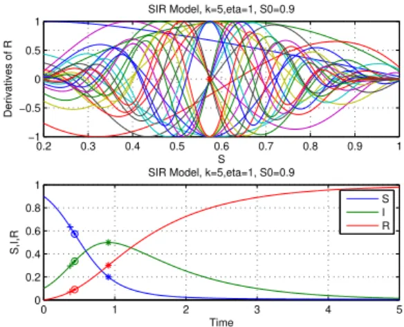
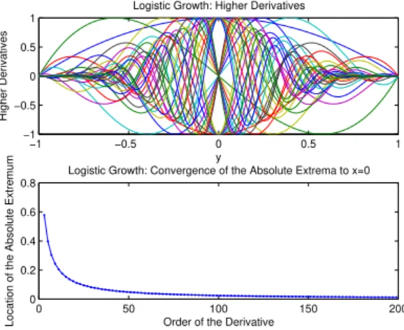
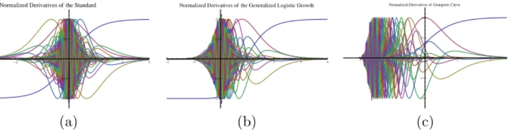
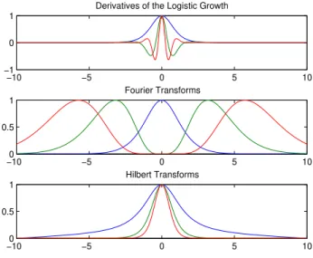
1.Introduction AyseHumeyraBilgeandYunusOzdemir Thecriticalpointofasigmoidalcurve

Kemal okuyor, yazıyor, postayı hazırlı­ yor, kavgaları yatıştırıyor, Muhbir doğruyu söylemekten ayrılınca Hürriyet’ i çıkarıyor. A v­ rupa’ya Avrupa’

Among them, the most symptomatic are the following: the inability of individual countries on their own to solve global problems; a high level of inter-civilization

Whenever in any country, community or on any part of the land, evils such as superstitions, ignorance, social and political differences are born, h u m a n values diminish and the

were also borrowed from Hungarian. A contradiction can immediately be noticed. Whereas [6] suggests that the sabre was used by the Magyars already before the Conquest, i.e. that

Existence and uniqueness of solutions of the Dirichlet Problem for first and second order nonlinear elliptic partial dif- ferential equations is studied.. Key words:

Therefore, a need to conduct an empiric study with students to get data for informing the mathematics education researchers about the situations of teacher practices and

“giving a high/desert salary”, “having healthy conditions, being hygienic” and “having regular breaks and regular working hours” are examined, it is seen that

According to the inquiry, we may point out that ap- plications of the transportation systems have a signifi- cant effect on the evolution of the city image in the case of