Date of publication xxxx 00, 0000, date of current version xxxx 00, 0000. Digital Object Identifier 10.1109/ACCESS.2017.Doi Number
Unsupervised Anomaly Detection in Multivariate Spatio-Temporal
Data using Deep Learning: Early Detection of COVID-19 Outbreak
in Italy
YILDIZ KARADAYI1, MEHMET N. AYDIN2, A. SELÇUK ÖĞRENCİ,3 Senior Member, IEEE
1Computer Engineering, Kadir Has University, Istanbul, Turkey 2Management Information Systems, Kadir Has University, Istanbul, Turkey 3Electrical-Electronics Engineering, Kadir Has University, Istanbul, Turkey
Corresponding author: YILDIZ KARADAYI (e-mail: [email protected]; [email protected]).
ABSTRACT Unsupervised anomaly detection for spatio-temporal data has extensive use in a wide variety of applications such as earth science, traffic monitoring, fraud and disease outbreak detection. Most real-world time series data have a spatial dimension as an additional context which is often expressed in terms of coordinates of the region of interest (such as latitude - longitude information). However, existing techniques are limited to handle spatial and temporal contextual attributes in an integrated and meaningful way considering both spatial and temporal dependency between observations. In this paper, a hybrid deep learning framework is proposed to solve the unsupervised anomaly detection problem in multivariate spatio-temporal data. The proposed framework works with unlabeled data and no prior knowledge about anomalies are assumed. As a case study, we use the public COVID-19 data provided by the Italian Department of Civil Protection. Northern Italy regions’ COVID-19 data are used to train the framework; and then any abnormal trends or upswings in COVID-19 data of central and southern Italian regions are detected. The proposed framework detects early signals of the COVID-19 outbreak in test regions based on the reconstruction error. For performance comparison, we perform a detailed evaluation of 15 algorithms on the COVID-19 Italy dataset including the state-of-the-art deep learning architectures. Experimental results show that our framework shows significant improvement on unsupervised anomaly detection performance even in data scarce and high contamination ratio scenarios (where the ratio of anomalies in the data set is more than 5%). It achieves the earliest detection of COVID-19 outbreak and shows better performance on tracking the peaks of the COVID-19 pandemic in test regions. As the timeliness of detection is quite important in the fight against any outbreak, our framework provides useful insight to suppress the resurgence of local novel coronavirus outbreaks as early as possible.
INDEX TERMS Spatio-temporal anomaly detection, multivariate, unsupervised, deep learning, COVID-19, outbreak detection, Italy.
I. INTRODUCTION
An anomaly is an observation whose properties are significantly different from the majority of other observations under consideration, which are called the normal data. Anomaly detection refers to the problem of finding these observations in data that do not conform to expected or normal behavior. A spatial-temporal outlier (ST-Outlier) is an object whose behavioral (spatial and non-temporal) attributes are significantly different from those of the other objects in its spatial and temporal neighborhoods [1]. Spatio-temporal data are extremely common in many problem settings where collecting data from various spatial locations at different times for the nature of the problem are
important. In such settings, detection of ST-Outliers can lead to the discovery of unexpected and interesting knowledge such as local instability and deformations [2]. Some examples of such spatio-temporal datasets are as follows: meteorological data, traffic data, earth science, and disease outbreak data. Events that generate spatio-temporal data are evolving events, such as hurricanes and disease outbreaks, and both spatial and temporal continuity are important in modelling such events [3].
For a problem domain, obtaining the labelled training data for all types of anomalies is often too expensive if not impossible [4]. This highlights the need for unsupervised techniques to find spatio-temporal anomalies. Moreover,
spatio-temporal datasets are generally multivariate, and have many contextual structures in them (spatial and temporal regularities), which makes them particularly difficult for labelling and well suited for unsupervised learning models. In the unsupervised scenarios, the type of anomalies and the ratio of anomalous events within the given dataset are generally not known. In such scenarios, we need to model the normal behavior of the underlying system in the presence of noise and anomaly which pose extra difficulty.
In this study, we address these challenges by proposing a hybrid deep learning framework. It is an autoencoder based anomaly detection framework. The hybrid framework structure is based on the idea of combining various deep neural network components. It has been successfully applied to multivariate time series forecasting [5], face detection [6], and video classification [7]. However, it has not yet been applied to unsupervised anomaly detection problem for non-image multivariate spatio-temporal data. Our proposed framework is composed of three stages: The first stage is the pre-processing of the multivariate spatio-temporal data so that the deep autoencoder network can exploit the spatial and temporal contexts jointly. The second stage is the data reconstruction stage, which is executed by a deep hybrid autoencoder network. The third stage is the anomaly detection stage, which is performed based on the reconstruction error. The hybrid autoencoder network is composed of a 3D convolutional neural network (CNN) based spatio-temporal encoder and a convolutional Long Short-Term Memory (ConvLSTM) network-based spatio-temporal decoder. It is designed to be trained in a truly unsupervised fashion for anomaly detection in non-image spatio-temporal datasets. We know that in a time series data set, data points with two adjacent timestamps are likely to have a higher similarity than data points with more distant timestamps. It is also true for spatio-temporal datasets that neighboring regions may have some strongly positively correlated patterns, such as traffic jam, climate change, and human activity. The hybrid deep learning framework is able to exploit contextual features of neighboring regions for anomaly detection in the absence of labels for normal or abnormal events.
The world has been fighting a pandemic caused by a new type of coronavirus (SARS-CoV-2) since it was discovered in China in December 2019. Almost all countries have been affected by the novel coronavirus (COVID-19) outbreak, and Italy is one of the hardest-hit European countries. As of May 15, the total number of positive cases reached 223,885 and the number of deaths exceeded 31,000. Following the identification of the first infections on the second half of February 2020 in northern Italy, authorities put an increasing number of restrictions in place [8]. Due to the high contagiousness of the infection, this did not stop further spreading of the epidemic by asymptomatic people. The peaks of the epidemic were delayed in Central and Southern Italian regions as expected compared to Lombardy and other northern regions [9]. As it has been shown by the COVID-19 outbreak, the biggest challenge is to detect the outbreak
during its early stages and mitigate its effects. The lack of an early epidemic warning system eliminated the opportunity to prohibit the epidemic spread at the initial stage. We would like to apply the proposed hybrid framework to tackle the problem of early disease outbreak detection in the midst of this global health crisis.
There have been many studies that model the epidemiological dynamics of COVID-19 [10]-[16]. They use either SEIR or other statistical models to predict the spreading and peaks of the epidemic, duration of the epidemic, and an overall number of potentially infected individuals at a national or regional level. However, none of those studies have focused on building an anomaly detection system for early epidemic detection. We believe that the proposed deep learning-based anomaly detection framework will prove useful in detecting COVID-19 epidemic waves. According to an analysis by disease experts, cases may come in waves of different heights by the end of 2021 depending on control measures and other factors [17]. This makes it quite necessary to build a monitoring tool for the timely detection of COVID-19 waves in different regions.
For any anomaly detection algorithm to be successful in early detection of disease outbreaks, it must incorporate both spatial and temporal aspects of a disease [18]. On the other hand, accurate monitoring of the evolution of the COVID-19 epidemic becomes extremely meaningful for the decision-making authorities to take appropriate actions against any public health crisis. As the extreme timeliness of detection is the new requirement of public health [19], this data-driven approach may help us build an anomaly detection tool for a more timely detection of the COVID-19 outbreak.
We use public COVID-19 data provided by the Italian Department of Civil Protection [20] as a case study in this research. We test the proposed model with the dataset at a resolution of the region level. We train one unified model with the data from northern regions, and using that model, we track the progression of the COVID-19 epidemic in test regions, which are central and southern regions of Italy. The framework can detect anomalous trends in test regions, which may signal the possibility of an outbreak. The main assumption here is that the data generated by northern regions' experience going through the epidemic can be used to derive an anomaly detection model. We evaluate the performance of the proposed framework against various univariate and multivariate methods including state-of-the art deep learning-based approaches proposed in recent years. Our framework has outperformed the state-of-the-art anomaly detection models in all test cases.
The main contributions of this study are the following: 1) To the best of our knowledge, the proposed approach,
which is composed of a novel data crafting and a hybrid deep learning model, is the first attempt in solving unsupervised anomaly detection problem in non-image multivariate spatio-temporal data.
2) It achieves good generalization capabilities in scenarios where the training data are scarce and contaminated with anomalies. In the case study, only
82 daily data entries (data points) are available for each region. Even these contaminated outbreak data are sufficient to build a robust anomaly detection model due to its effective architecture to exploit spatial neighborhood data.
3) The biggest challenge in anomaly detection for spatio-temporal data is to combine the contextual attributes in a meaningful way. In the proposed hybrid approach, spatial and temporal contexts are handled by different deep learning components as these contextual variables refer to different types of dependencies.
4) The proposed hybrid framework is designed to be trained in a truly unsupervised fashion without any labels indicating normal or abnormal data. The architecture is robust enough to learn the underlying dynamics even if the training dataset contains noise and anomalies.
The rest of the paper is organized as follows. Section II provides an overview of existing methods for anomaly detection. Traditional anomaly detection methods are discussed in part A of Section II, whereas the state-of-the-art deep learning-based anomaly detection methods are mentioned and summarized in part B of Section II. Section III provides the related background information on traditional autoencoders and autoencoder based anomaly detection. The methodology including the problem formulation and the design of the proposed hybrid deep learning framework is presented in Section IV. Experiments and results are presented in Section V. Finally, Section VI concludes the paper and gives the directions for possible future work.
II. RELATED WORK
A. TRADITIONAL APPROACHES
The task of detecting outliers or anomalous events in data has been studied extensively in the context of time series and spatial data separately. Time-series outlier detection studies find outliers considering only temporal context [21], [22]. For data with spatial context, several context-based anomaly detection techniques have been proposed [23]-[26]. In geoscience and environmental research, some statistical and simulation-based methods have been proposed for spatial anomaly detection [27], [28]. For spatio-temporal outlier detection, both spatial and temporal continuity should be considered for modeling. Hence, spatio-temporal outlier detection methods are significantly more challenging because of the additional difficulty of modeling the temporal and spatial components jointly [2], [3].
Distance and density-based outlier detection algorithms have also been applied to anomaly detection problems in spatial datasets, such as Local Outlier Factor (LOF) [29], [30], and DBSCAN [31]. LDBSCAN algorithm [32], created by the merge of DBSCAN and LOF, is a density-based algorithm for unsupervised anomaly detection problems in spatial databases with noise. Another popular proximity-based outlier detection approach is based on cluster analysis. The non-membership of
a data point to any of the clusters can be used as a sign of being outlier [33]. Cluster-Based Local Outlier Factor (CBLOF) [34] is a clustering-based anomaly detection algorithm, in which the anomaly score of an instance is the distance to the next large cluster. Choosing the right number of clusters is very important since all clustering methods tend to be very sensitive to this choice.
In [35], Birant and Kut propose a neighborhood-based ST-Outlier detection algorithm. They use a modified version of DBSCAN algorithm to identify the spatial neighborhoods within the dataset. They define spatial outliers based on these neighborhoods. Then, they check the temporal context of spatial outlier objects by comparing them to temporal neighbor objects. However, their algorithm does not generate a score for data points. In [2], Cheng and Li propose a four-step approach to identify spatio-temporal outliers: classification (clustering), aggregation, comparison and verification. In [36], Gupta et al. introduce the notion of context-aware anomaly detection in distributed systems by integrating the information from system logs and time series measurement data. They propose a two-stage clustering methodology to extract context and metric patterns using a PCA-based method and a modified K-Means algorithm.
The aforementioned spatio-temporal anomaly detection methods have something in common: They first apply spatial (or non-temporal) context to find spatial outliers using a distance-based technique. Then, spatial outliers are compared with other spatial objects using temporal neighborhoods to identify if they are temporal outliers too. They do not combine the contextual (spatial and temporal) attributes in a meaningful way as these attributes refer to different types of dependencies. Despite the inherent unsupervised settings of distance and cluster-based algorithms, they may still not detect anomalies effectively due to the following reasons:
1) In multivariate time series data, strong temporal dependency exists between time steps. Hence, distance-/cluster-based methods, may not perform well since they cannot capture temporal dependencies properly across different time steps.
2) The definition of distance between data points in multivariate spatio-temporal data with mixed attributes is often challenging. This difficulty may have an adverse effect on outlier detection performance of distance-based clustering algorithms.
3) Another problem with distance-based methods is that they are well known to be computationally expensive and not suitable for large datasets.
IsolationForest [37], [38] is a powerful approach for anomaly detection in multivariate data without relying on any distance or density measure. In particular, it is an unsupervised, tree-based ensemble method that applies the novel concept of isolation to anomaly detection. It detects anomalies based on a fundamentally different model-based approach: an anomalous point is isolated via recursive partitioning by randomly selecting a feature, and then
randomly selecting a split value for the selected feature. The output is the anomaly score for each data point. Although it establishes a powerful multivariate non-parametric approach, it works on continuous-valued data only. Numenta HTM [39], [40] is an unsupervised anomaly detection method for univariate streaming data based on Hierarchical Temporal Memory (HTM). It works based on the multiple predictions for the next time step which is done by a layer of HTM neurons. Anomaly score is generated based on the likelihood of the prediction error, which is a probabilistic metric defining how anomalous the current state is, based on prediction history. One-class SVM (OCSVM), which is a semi-supervised anomaly detection technique, has been applied extensively to anomaly detection problems in time series data [41] - [43]. However, OCSVM is sensitive to the outliers especially when used in an unsupervised fashion when there are no labels.
Several algorithms proposed in the statistics literature have been used widely for time series prediction and anomaly detection such as autoregressive integrated moving average (ARIMA) and Exponentially Weighted Moving Average (EWMA) [44] - [47]. Most detection algorithms in bio-surveillance which operate on univariate time series data have been taken from the field of quality control [48]. The common techniques include control charts [49] and CUmulative SUM Statistics (CUSUM) [47], [50]. What’s Strange About Recent Events (WSARE) [48] algorithm was developed for syndromic surveillance to the hospital setting, such as symptoms exhibited by patients at an Emergency Department (ED). WSARE is a rule-based algorithm specifically designed for patients’ pre-clinical data. It combines two approaches: association rule mining and Bayesian networks. Although the WSARE algorithm works on multidimensional data, it can only be used on categorical data sets. The Spatial Scan Statistic [51] can be considered the real-valued analog of WSARE. However, it is computationally expensive for large data sets. Neill and Cooper [52] proposed the multivariate Bayesian scan statistic (MBSS) for event detection in multivariate spatial time series data. However, their approach requires the prior probability of each event occurring in each space-time region. They need either an expert knowledge or labeled data to obtain the prevalence of each event type.
B. DEEP LEARNING BASED APPROACHES
Besides traditional anomaly detection methods, deep learning-based anomaly detection approaches have recently gained a lot of attention. In the literature, artificial neural networks have been widely applied to anomaly detection tasks for various types of datasets [53]. Reconstruction based and prediction based deep learning models are among the most widely used architectures for anomaly detection in videos and time-series data [54], [55].
Malhotra et al. [56] proposes a deep Long Short-Term Memory (LSTM) network to detect anomalies in univariate time series. They use LSTM network architecture to predict
next l steps of the input. Then, the prediction error is used to detect anomalies. The model is trained using normal data to learn the Gaussian distribution of error vectors. Malhotra et al. [57] propose an LSTM network-based encoder-decoder scheme for anomaly detection in univariate time series datasets. Their model learns to reconstruct ‘normal’ time series data and uses reconstruction error to detect anomalies. Hasan et al. [58] propose a deep fully convolutional autoencoder to reconstruct the input sequence of video frames to detect anomalies. The network is trained in semi-supervised fashion with regular videos. It learns the signature of each frame in regular motion videos. An anomaly score of each frame in the test set is then calculated based on reconstruction error.
Various deep learning-based feature extraction methods have been proposed in the literature. The proposed architectures are used to extract useful (discriminative) features for anomaly detection, novelty detection or classification problems. Yang et al. [59] present a CNN-LSTM based recurrent autoencoder network for unsupervised extraction of highlights in video data, whereas in [60] a pre-trained 3D convolutional network is used to extract features from video segments for anomaly detection process. Munawar et al. [61] build an encoder composed of deep convolutional neural network and Restricted Boltzman Machine to extract features from videos. The extracted features are fed into an LSTM based prediction system to predict the next video frame in the learned feature space. Then, the difference between the prediction and actual observation in the feature space is used to detect anomalies. In a recent study, Perera and Patel [62] propose a one-class transfer learning schema for feature extraction based on Convolutional Neural Network (CNN). Estiri and Murphy [63] use a semi-supervised deep autoencoder for outlier detection in multivariate clinical observation data from Electronic Health Records (EHR).
D’Avino et al. [64] propose an LSTM-based autoencoder framework to detect forgeries in video frames. They train their model with pristine frames without any forgeries. They use reconstruction errors to detect any abnormalities in the frames with spliced areas. Chong and Tay [65] propose a spatiotemporal architecture for anomaly detection in videos. Their autoencoder based anomaly detection framework contains a spatial feature extractor and temporal encoder-decoder component. The spatial encoder component comprises two convolutional and two de-convolutional layers. They use a three-layer convolutional long short-term memory (LSTM) network as temporal encoder-decoder component. Munir et al. [66] present DeepAnT, a deep learning based unsupervised anomaly detection approach for time series data. DeepAnT architecture is based on 1D deep convolutional neural network to predict univariate time series data. They use the prediction-based approach where a window of time series is used as a context and the next time stamp is predicted. The anomaly detector module uses the prediction error and a pre-defined threshold value to tag each data point as normal or
abnormal. Nogas et al. [67] use a deep spatio-temporal convolutional autoencoder schema, DeepFall, to detect falls in videos. They formulate the fall detection problem as one class classification problem. Their classification framework consists of a 3D convolutional autoencoder for learning spatio-temporal features from video frames. They use semi-supervised learning approach that their model is trained only on the videos with normal activities of daily living without fall frames in them. Then, they use annotated video data to detect fall frames which are considered abnormal.
Despite the effectiveness of those abovementioned deep learning approaches, they are either supervised or semi-supervised models. In the semi-supervised approaches, models need labels for all targeted anomaly classes for training. In the semi-supervised approaches, models use only normal data to model the majority class (normal class) to further detect future anomalies. The proposed framework is designed to be trained in a truly unsupervised fashion without any labels indicating normal or abnormal data. The architecture is robust enough to learn the underlying dynamics even if the training dataset contains noise and anomalies. The main distinction between other deep learning based methods and the proposed hybrid approach is that they perform on either multivariate time series data or video data, and none of them is actually designed for non-image spatio-temporal multivariate datasets with both spatial and temporal contextual attributes.
III. BACKGROUND
A. AUTOENCODERS
Autoencoders are commonly used for dimensionality reduction of multidimensional data as a powerful non-linear alternative to PCA or matrix factorization [68] – [70]. If a linear activation function is used, the autoencoder becomes virtually identical to a simple linear regression model or PCA/matrix factorization model. When a nonlinear activation function is used, such as rectified linear unit (ReLU) or a sigmoid function, the autoencoder goes beyond the PCA, capturing multi-modal aspects of the input distribution [71], [72]. It is shown that carefully designed autoencoders with tuned hyperparameters outperform PCA or K-Means methods in dimension reduction and characterizing data distribution [73], [74]. They are also more efficient in detecting subtle anomalies and in computation cost than linear PCAs and kernel PCAs respectively [75].
A traditional autoencoder is a feed-forward multi-layer neural network which is trained to copy its input into the output. To prevent identity mapping, deep autoencoders are built with low dimensional hidden layers by creating non-linear representation of input data [68]. Usually, an autoencoder with more than one hidden layer is called a deep autoencoder [76]. Deep autoencoders have been successfully applied to dimensionality reduction, image denoising, and information retrieval tasks [77], [78].
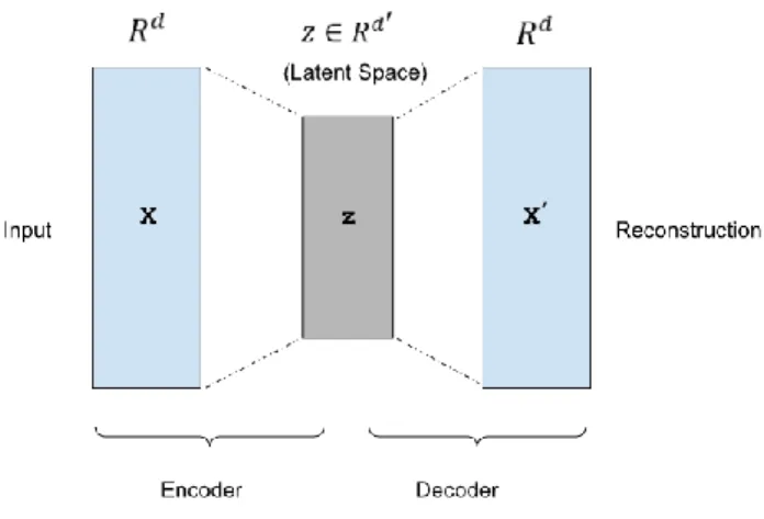
FIGURE 1. Illustration of an autoencoder.
An autoencoder is trained to encode the input 𝑥 into some latent representation 𝑧 so that the input can be reconstructed from that lower dimensional representation. An autoencoder is usually trained using back-propagation in an unsupervised manner, to learn how to build its original input by minimizing the reconstruction error of the decoding results. Fig. 1 depicts a typical autoencoder network structure with one hidden layer. They are composed of two parts: an encoder and a decoder. Deep autoencoders learn a non-linear mapping from the input to the output through multiple encoding and decoding steps. An autoencoder takes an input vector 𝑥 ∈ 𝑅𝑑, and first maps it to a latent representation 𝑧 ∈ 𝑅𝑑′ through a mapping:
𝑧 = 𝑓𝜃(𝑥) = 𝑊𝑥 + 𝑏 (1) where the function 𝑓𝜃 represents encoding steps and parameterized by 𝜃 = {𝑊, 𝑏}. 𝑊 is a 𝑑′× 𝑑 weight matrix and 𝑏 is a bias vector. The lower dimensional latent representation of the input is then mapped back to a reconstructed vector 𝑥′∈ 𝑅𝑑 in the input space:
𝑥′= 𝑔
𝜃′(𝑧) = 𝑊′𝑧 + 𝑏′ (2)
where the function 𝑔𝜃′ represents decoding steps and parameterized by 𝜃′= {𝑊′, 𝑏′}. The autoencoders training procedure consists of finding a set of parameters {𝑊, 𝑏, 𝑊′, 𝑏′} that make the reconstructed vector 𝑥′ as close as possible to the original input 𝑥. The parameters of autoencoder are optimized by minimizing a loss function that measures the quality of the reconstructions. The loss function of an autoencoder is sum-of-squared differences between the input and the output:
∑ ∑𝑑 ||𝑥𝑖− 𝑥′𝑖||2 𝑖=1
𝑥∈∅ (3)
where ∅ is the training dataset.
B. ANOMALY DETECTION WITH AUTOENCODERS
The main idea behind autoencoder based anomaly detection is to measure how much the reconstructed data deviates from the original data. An autoencoder has an unsupervised
learning objective whose primary task is to copy the input to the output [77]. Therefore, an autoencoder is trained to reconstruct data by minimizing this objective function, or loss function. For anomaly detection, reconstruction error is used as the anomaly score. Data points which generate high reconstruction errors can be categorized as anomalous data points based on a threshold value. When autoencoders are used for anomaly detection, they are trained using only normal data instances as we have abundance of normal data. The training dataset should be cleaned from anomalous data points and outliers as much as possible for a successful model generation. After the training process, the autoencoder will generally reconstruct normal data with very small reconstruction error. As the autoencoder has not encountered the abnormal data during the training, it will fail to reconstruct them and generate high reconstruction errors which can be used as anomaly score [71], [75].
There are some practical issues in using autoencoders with contaminated training data (dataset with normal and anomalous data points). Since anomalies are treated as normal data points during the training phase, there will be inevitably more errors in the model compared to training with only normal data points. If we try to overcome these errors by tuning the network with more layers and neurons, we may face the problem of overfitting which is a significant problem in the case of deep neural networks. A sufficiently complex deep autoencoder may even learn how to represent each anomaly with sufficient training by generating low reconstruction errors which would be a problem in anomaly detection [71].
IV. METHODOLOGY
A. PROBLEM FORMULATION
A univariate time series is a sequence of real valued data points with timestamps. A multivariate time series is a set of univariate time series with the same timestamps. In this paper, we focus on multivariate time series that are measured at successive points in time, spaced at uniform time intervals.
Let 𝑋 = {𝑥(𝑛)} 𝑛=1
𝑁 denote a multivariate time series dataset composed of N data points. Let each data point 𝑥(𝑛) has T time steps, and each observation at time step t, is a d dimensional vector. The dataset X has dimensions of (d, T), where 𝑥(𝑛) ∈ ℝ𝑑×𝑇. Each data point 𝑥(𝑛) is a two-dimensional data matrix and can be represented as:
𝑥(𝑛) = (
𝑥11𝑛 ⋯ 𝑥1𝑇𝑛
⋮ ⋱ ⋮
𝑥𝑑1𝑛 ⋯ 𝑥𝑑𝑇𝑛
) (4) The superscript 𝑛 represents the ordered number of each data point within the dataset X. 𝑥(𝑛) is a multivariate time series data point with a contextual time attribute. Each 𝑥(𝑛) in the dataset 𝑋 is ordered based on the timestamp. As the number 𝑛 increases, the time context changes, and time dimension, or timestamps, moves ahead.
In a spatio-temporal dataset, each multivariate data point 𝑥(𝑛) comes from a different spatial location, or region, which
has different spatial attributes (such as latitude and longitude). We denote the multivariate spatio-temporal dataset as DST =
{(𝑋(𝑖), 𝑆(𝑖))}𝑖=1𝑚 which contains multivariate time series data points from m different spatial regions. Each spatial region 𝑆𝑖, where 𝑆𝑖 Є S, has a set of multivariate time series data represented by the dataset 𝑋(𝑖). 𝑁(𝑖) represents the number of data points (or observations) in each spatial region 𝑆𝑖. In other words, it is the size of 𝑋(𝑖), which may be different for each region in real-world scenarios.
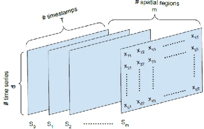
𝑋𝑆𝑇, which is the multivariate spatio-temporal data matrix, can be represented as a 3-dimensional tensor as shown in Fig. 2. It is built using multivariate time series data from 𝑚 different spatial regions or 𝑆𝑖s, where 𝑖 = 1 … 𝑚. The sliding window technique which is used to build the 3-dimensional data matrix 𝑋𝑆𝑇, is given in Algorithm 1. It is composed of 𝑚 multivariate time series data points from 𝑚 different spatial regions and representing observations from the same time window with the same timestamps. 𝑇, which is called the “input window-size”, represents the number of timestamps in the multivariate data point, and 𝑑 represents the number of univariate time series. 𝑚 represents the number of nearest spatial neighborhood to include in the anomaly detection process. The best 𝑚 can be found empirically for each problem domain. The 𝑚 number of nearest neighboring regions are selected from S different regions based on the pairwise spatial distance between regions.
FIGURE 2. 3-dimensional multivariate spatio-temporal data matrix structure used in anomaly detection procedure.
We formulate the spatio-temporal anomaly detection problem as detecting anomalous multivariate observations (sample of 𝑥(𝑖) data points) in the dataset D
ST which
differentiate significantly from their spatial and temporal neighbors. Given the spatio-temporal 3-dimensional data matrix 𝑋𝑆𝑇, the goal is to reconstruct the multivariate-time series data from the region 𝑆𝑖, where 𝑆𝑖∈ 𝑆. 𝑆𝑖 represents the target region or the region of interest in which spatio-temporal anomalies are investigated. Anomalous data points have large reconstruction errors because they do not conform to the subspace patterns in the data. Therefore, the aggregated reconstruction errors over the time dimension 𝑇 can be used
as the anomaly score for the autoencoder based proposed framework. All 𝑥𝑖(𝑛) multivariate data points, or sub sequences, with high reconstruction errors from the region 𝑆𝑖 are considered to be anomalies.
B. PROPOSED HYBRID FRAMEWORK
The proposed approach consists of three main stages: The first stage is the data pre-processing stage. At this stage, the multivariate spatio-temporal dataset is processed in such a way that the deep autoencoder network can exploit the spatial and temporal contexts jointly. Multivariate data from 𝑚 nearest spatial neighbors are used to represent spatial dependency between different spatial regions. The sliding window technique given in Algorithm 1 is applied to build the multivariate spatial-temporal input data for the framework. By using the multistep overlapping subsequences from 𝑚 nearest spatial neighborhood of each data point, we build a 3-dimensional data matrix as shown in Fig. 2, which can represent the spatial and temporal dependency within the dataset.
The important parameters of this algorithm are window size T and step size s. They should be chosen carefully based on the underlying dynamics of each dataset and the goal of anomaly detection problem at hand. The length of each subsequence is equal to the window size. Using sliding window technique, for a long sequence with length L, the number of extracted subsequences can be given as:
num. of subseq. = ⌈(𝐿 − 𝑇 + 1)/𝑠⌉ (5) which gives the maximum number of subsequences we can possibly extract for a given T and s.
The second stage is the data reconstruction stage which is executed by the deep hybrid autoencoder network. The proposed hybrid autoencoder network consists of two main components: a spatio-temporal encoder component which has a 3D convolutional neural network (CNN), and a spatio-temporal decoder component which has a Convolutional Long Short-term Memory (ConvLSTM) network.
The third stage is the anomaly detection stage. The anomaly detection is performed by calculating the reconstruction error as anomaly score. Let 𝑥 = {𝑥(1), 𝑥(2), … , 𝑥(𝑇)} be a univariate time series data representing one of the reconstructed features and 𝑇 is the length of the input window. Each data point 𝑥(𝑖) represents a data reading for that feature at time instance 𝑡𝑖. The mean absolute error (MAE) is used to calculate the reconstruction error for the given time period (input window) for each feature as:
𝑒𝑀𝐴𝐸(𝑥) = 1
𝑇 ∑ |𝑥T 𝑖− 𝑥̂𝑖| (6) where 𝑥𝑖 is the real value and 𝑥̂𝑖 is the reconstructed value at time instance 𝑡𝑖. The reconstruction error for each feature and for all data points in the test set is calculated. Each data point in the test set represents a window of size 𝑇 as the
rolling window. As each data point in the dataset is generated using sliding window algorithm with step size set to s, we generate rolling window estimation, and hence the rolling window errors.
For an anomaly detection problem, we are only interested with the reconstruction of a subset of original spatio-temporal multivariate dataset and not the fully reconstructed version of it. The overall framework is trained to produce the target multivariate time series 𝑋 = {𝑥1, … , 𝑥𝑇′} of length 𝑇′ which is the size of the reconstruction window. The length of 𝑇′ can be equal to or smaller than the input window size 𝑇 and should be tuned for each problem. Each sequence 𝑥𝑖 ∈ ℝ𝑑
′
is an 𝑑′-dimensional vector where 𝑑′≤ 𝑑.
C. SPATIO-TEMPORAL ENCODING
The encoder component uses 3D convolutions to capture complex spatial dependencies in each spatial neighborhood. By convolving a 3D kernel over the cube formed data, the encoder can extract better representative features. The cuboid data is formed by stacking the data from the nearest spatial neighbors of each data point as explained in Algorithm 1. This allows information across these spatially close neighbors to be connected to form feature maps, thereby capturing spatio-temporal information encoded in the close neighborhood.
In most typical CNNs for image recognition, the input data is a single image with three channels for color images (R, G and B color channels) or one channel for grayscale images. In anomaly detection networks, the input data is generally a video clip consisting of multiple frames. In convolutional autoencoder based applications, T frames in the channel dimension are stuck, and then fed into the autoencoder where T is the length of the sliding window. In the case of 2D convolutional autoencoders, the temporal features are rarely preserved as 2D convolution operations are performed only spatially [58].
In this study, 3D convolutional operations are applied on multivariate spatio-temporal data to better preserve the temporal features along with the spatial features. The input data are re-constructed as a 3-dimensional cuboid by stacking multivariate data frames as illustrated in Fig. 2. By applying this idea, we can accomplish dimensionality reduction both in spatial and temporal context for a given input window during the encoding phase. The main component of the spatio-temporal encoder is the 3D convolutional layer, which is defined as follows: the value 𝑣 at position (𝑥, 𝑦, 𝑧) of the 𝑗 th feature map in the 𝑖th 3D convolutional layer, with bias 𝑏𝑖𝑗, can be written by the following equation [79]: 𝑣𝑖𝑗𝑥𝑦𝑧= 𝑓 (∑ ∑ ∑ ∑ 𝑤𝑖𝑗𝑚𝑝𝑞𝑠𝑣(𝑖−1)𝑚(𝑥+𝑝)(𝑦+𝑞)(𝑧+𝑠)+ 𝑏𝑖𝑗 𝑆𝑖−1 𝑠=0 𝑄𝑖−1 𝑞=0 𝑃𝑖−1 𝑝=0 𝑚 ) (7)
where 𝑃𝑖, 𝑄𝑖, and 𝑆𝑖 represent the vertical (temporal depth, or window size, T), horizontal (temporal width, or number of
features, d), and spatial depth (number of spatial neighbors, m) dimensions of the kernel cube 𝑤𝑖 in the 𝑖th layer. The set of feature maps from the (𝑖 − 1)th layer is indexed by 𝑚, and 𝑤𝑖𝑗𝑚𝑝𝑞𝑠 is the value of the kernel cube at the position 𝑝𝑞𝑠 connected to the 𝑚th feature map in the previous layer. The number of feature maps is defined by the number of kernel cubes at each convolution layer.
C. SPATIO-TEMPORAL DECODING
For the decoding part of the framework, we use convolutional LSTM (ConvLSTM) network, which is a variant of LSTM network. It has been introduced by Shi et al. [80]. It has been recently utilized by Chong and Tay in [65] for abnormal event detection in videos and by Patraucean et al. in [81] for motion estimation in videos.
The major drawback of regular Long Short-Term Memory (LSTM) networks is that they are not capable of preserving the spatial information during the state transitions [80]. To overcome this problem, ConvLSTM units have convolutions operations in place of matrix operations in all gates and cell outputs. As they use convolution for both input-to-hidden and hidden-to-hidden connections, they require fewer weights and yield better spatio-temporal feature encoding and decoding performance. The formulation of a ConvLSTM unit can be given by the following equations from (8) through (13):
𝑓𝑡= 𝜎(𝑊𝑓∗ [𝑋𝑡, 𝐻𝑡−1, 𝐶𝑡−1] + 𝑏𝑓) (8) 𝑖𝑡= 𝜎(𝑊𝑖∗ [𝑋𝑡, 𝐻𝑡−1, 𝐶𝑡−1] + 𝑏𝑖) (9) 𝐶̂𝑡= 𝑡𝑎𝑛ℎ(𝑊𝐶∗ [𝑋𝑡, 𝐻𝑡−1] + 𝑏𝐶) (10) 𝐶𝑡= 𝑓𝑡⊗ 𝐶𝑡−1+ 𝑖𝑡⊗ 𝐶̂𝑡 (11) 𝑜𝑡= 𝜎(𝑊𝑜∗ [𝑋𝑡, 𝐻𝑡−1, 𝐶𝑡−1] + 𝑏𝑜) (12) ℎ𝑡= 𝑜𝑡⊗ 𝑡𝑎𝑛ℎ(𝐶𝑡) (13) where ’∗’ denotes the convolution operator and ’ ⊗’ denotes the Hadamard product. Equation (8) represents the forget gate, (9) and (10) are the gates where new information (input 𝑋𝑡) is added, (11) combines the new and old information factored by the forget gate, whereas (12) and (13) give the output of the ConvLSTM unit for the next time step. The variable 𝑋𝑡 denotes the input vector, ℎ𝑡 denotes the hidden state, and 𝐶𝑡denotes the cell state for the time step 𝑡. 𝑊′s are the trainable weight matrices and 𝑏′𝑠 are the bias vectors.
V. EXPERIMENT
A. DATASET
We use the public Italian COVID-19 time series dataset provided by the Italian Department of Civil Protection. It can be downloaded from the website [82], which is constructed as a national response effort for coronavirus emergency. For this study, we use the regional dataset which shows the daily
progress of new coronavirus epidemic in regions of Italy. The regional dataset provides detailed epidemiological figures for all 21 regions (19 regions and 2 autonomous provinces) starting from February 24 and updated daily.
The regions dataset has 20 features as follows (translated into English): Date, country, region code, region name, latitude, longitude, hospitalized with symptoms, intensive care patients, total hospitalized patients, home isolation, total positives (current positives), change in total positive, new positives, recovered (discharged), deceased, total cases, tests performed, total number of people tested, notes in Italian, notes in English.
Features “date, country, region code, region name, latitude, longitude” are contextual attributes whereas the rest are regarded as behavioral attributes. The feature "tests performed" is part of the government intervention measures and shows significant differences between regions depending on the policies taken by each regional government in Italy [83]. As proactive testing and mobility can affect the epidemiological dynamics of the COVID-19 epidemic [84], it is regarded as contextual variable for the modelling, and is not included in the reconstruction space as a behavioral attribute.
All these features have been used during the modeling except the redundant and mostly empty attributes. The "total number of people tested" field is empty for most of the regions, so it is dropped for the modelling. Features "notes in Italian, notes in English, total number of people tested" are also discarded for this study as they are mostly empty. As the only country in the dataset is Italy, ‘country’ column is also dropped. On the website, the data format is explained as follows:
- total positives: Total amount of current positive cases (hospitalized patients + home confinement)
- change in total positive: New amount of current positive cases (total positives current day – total positives previous day)
- new positives: New amount of current positive cases (total cases current day – total cases previous day)
- total cases: Total amount of positive cases
Based on those detailed descriptions of dataset, we rename the feature "total positives" as "current positive cases" in our study to make the feature name more representative. We also regard the feature "new positives" as "daily confirmed new positive cases," and renamed it as "new positive cases" for clarity. In addition to the regional epidemic data, we have also used population data of each region from ISTAT website [85]. By using population information, we have calculated three additional features: "total positive cases, new positive cases and deaths" on each 10,000 inhabitants. Using these engineered features, we have incorporated the case density information on each region to enrich spatial data.
Latitude and longitude are also provided for each region making this regional dataset a spatiotemporal dataset. Daily epidemic data entry for each region has two contextual attributes: a date attribute (temporal context) and
latitude-longitude attributes (spatial context), which is static for each region. Besides these contextual attributes, the rest of the attributes including the engineered features are regarded as behavioral attributes. We use the min-max normalization method to scale all behavioral attributes in the dataset into the range of [0, 1] to accelerate the learning process and to avoid large weights which cause neural networks to overfit.
B. DATA PREPARATION
We use the regional data entries between February 24 and May 15, inclusively. The model is trained with the data from northern regions which provides a complete epidemiological data in the sense that they have gone through all the peaks of COVID-19 outbreak showing a complete perspective for anomaly detection. The training dataset contains data from following northern regions: P.A. Bolzano, Emilia-Romagna, Liguria, Lombardia, Piemonte, P.A. Trento, Valle d'Aosta, Veneto, and Friuli Venezia Giulia. We use data from one central region (Marche) as validation set; data from one central region (Lazio), one region from southern Italy (Campania), and one island region (Sicilia) as test set. The total data entry for each region is 82, which means 82 days of COVID-19 epidemiological data are entered for each region.
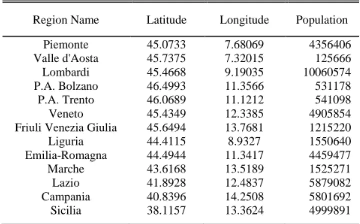
The spatial attributes of all regions used in this study is given in Table I. Using the latitude and longitude information, we calculate the distance matrix showing the pairwise distance of all regions used in this study. We use the haversine formula to calculate the shortest distance between regions, which is used to measure distances on a sphere [86].
TABLEI REGION INFORMATION
Region Name Latitude Longitude Population Piemonte 45.0733 7.68069 4356406 Valle d'Aosta 45.7375 7.32015 125666 Lombardi 45.4668 9.19035 10060574 P.A. Bolzano 46.4993 11.3566 531178 P.A. Trento 46.0689 11.1212 541098 Veneto 45.4349 12.3385 4905854 Friuli Venezia Giulia 45.6494 13.7681 1215220 Liguria 44.4115 8.9327 1550640 Emilia-Romagna 44.4944 11.3417 4459477 Marche 43.6168 13.5189 1525271 Lazio 41.8928 12.4837 5879082 Campania 40.8396 14.2508 5801692 Sicilia 38.1157 13.3624 4999891
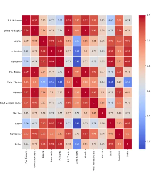
We calculate the correlation coefficients for the feature "current positive cases" between every pair of districts in the training data using Pearson correlation. The correlation heatmap matrix in Fig. 3 shows that all the neighboring regions have strong spatial correlations. Remote regions in the dataset, such as Valle d'Aosta and Marche, show weaker correlations between other regions. These results reflect that the spatial correlation of COVID-19 epidemic progression occurring in certain geographic regions at a certain spatial resolution is quite strong.
By using the spatial neighborhood of each region, we create a spatio-temporal multivariate input for the model. The sliding window technique given in Algorithm 1 is applied to training, validation, and test datasets to build spatio-temporal multivariate subsequences. We apply the algorithm with parameters representing the number of spatial neighbors (which is called depth in the algorithm) set to 10, the window size set to 7 representing 7-day worth of data point, and step size to 1. According to the formula given in (5) in which T is set to 7, s is set to 1 and L is set to 82, we have 76 multivariate subsequences for each region. As the total number of behavioral attributes is 13, excluding spatial features “region code, region name, latitude, and longitude”, and with the depth of spatial neighborhood is set to 10, we create 76x7x13x10 dimensional spatio-temporal multivariate dataset from each region. By using this sliding window algorithm, we perform data augmentation by moving the start of the T-day data entry by step size resulting in a nearly six-fold expansion of the training data.
The parameter "number of spatial neighbors" represents the number of nearest neighbors to use while building spatio-temporal multivariate subsequences. It also corresponds to the spatial dimension of the 3D CNN encoder. After data preprocessing step is completed, training, validation and test sets are created. They are 4-dimensional data matrices with the following sizes: The dimension of the training set is 684x7x13x10, the dimension of the validation set is 76x7x13x10, and the dimension of the test set is 228x7x13x10. Numbers 684, 76 and 228 represent the number of data points or observations in training, validation, and test sets, respectively. The proposed framework is trained to reconstruct the following behavioral attributes: Hospitalized patients, intensive care patients, total hospitalized patients, home confinement, current positive cases, new positive cases, total positive cases, recovered, and deaths. The size of the reconstruction space for the test set is 228x7x9.
C. FRAMEWORK ARCHITECTURE AND TUNING
Extensive experiments through grid search are executed to finalize the architecture of the framework and its hyperparameters. Specifically, we use 2 CNN blocks in the encoder component, each of which has a 3D convolutional layer, followed by a 3D max-pooling layer. Number of feature maps is set to 64 in the first block and set to 32 in the second block with padding and no striding (or with strides 1×1×1). We set the kernel size to 3 × 3 × 5, where 𝑃𝑖 = 𝑄𝑖 = 3 and 𝑆𝑖 = 5 in (7), for all convolutional layers for the experiment, as these values are found to produce the best result for the dataset. The max-pooling layers have pool size of 2 × 2 × 2 and strides of 1 × 2 × 2 with padding. This means that the pooling operation is performed over all three dimensions: (𝑡𝑒𝑚𝑝𝑜𝑟𝑎𝑙 𝑑𝑒𝑝𝑡ℎ × 𝑡𝑒𝑚𝑝𝑜𝑟𝑎𝑙 𝑤𝑖𝑑𝑡ℎ × 𝑠𝑝𝑎𝑡𝑖𝑎𝑙 𝑑𝑒𝑝𝑡ℎ). In addition, temporal width and spatial depth dimensions are reduced by a factor of 2 with every max-pooling layer. The activation function 𝑓 in (7) in all hidden convolutional layers in the encoder component are set to Rectified Linear Unit
(ReLU) non-linearity, 𝑅𝑒𝐿𝑈(𝑥) = max (𝑥, 0), which allows the deep neural networks converge faster [87].
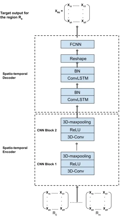
The decoder component is composed of two ConvLSTM layers with the number of feature maps set to 32 and 64, respectively to preserve the symmetry of the autoencoder framework. We apply 2D convolution operation over spatial and temporal dimensions using the kernel size of 3 × 2 and the stride of 1 × 1 with padding. Batch normalization (BN) [88] is applied to each of the ConvLSTM layers, which accelerates the training of deep neural networks. In the final layer, a fully connected neural network (FCNN) is used to reconstruct the target output. Thus, we add a layer to reshape the 4D output of final ConvLSTM layer before passing the output to the FCNN. The FCNN layer is a time distributed dense layer which applies the same fully connected operation to every time step. The number of units in the dense layer is set to 𝑑′= 9 and it is equal to the number of univariate time series (features) that we want to reconstruct. The number of hidden units in the FCNN layer can be adjusted according to the problem context at hand.
Activation functions of ConvLSTM units are set to hyperbolic tangent and the activation functions in the final dense layer are set to ReLU. Layer weights are initialized with the Glorot uniform initializer [89]. The deep learning framework is optimized using the Adam optimizer with learning rate set to 0.0001. It ran for 100 epochs with batch size 16. The training is regularized by weight decay (the 𝐿2 penalty multiplier set to 1 × 10⁻⁴) and dropout regularization for the two ConvLSTM layers (the dropout ratio set to 0.25). The model is trained to minimize the following mean absolute error (MAE) loss function:
𝑀𝐴𝐸 =
1𝑛
∑
|𝑥
𝑖− 𝑥̂
𝑖|
𝑛𝑖=1 (14)
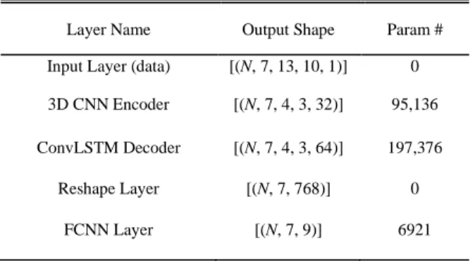
where 𝑥𝑖 and 𝑥̂𝑖 represent the true value and the reconstructed value, respectively, and 𝑛 is the total number of data points in each batch. The detailed architecture of the final deep learning framework is illustrated in Fig. 4. The final framework has 299,241 trainable parameters. The data structure of each component in the trained framework is given in Table II, where N represents number of data points.
TABLEII FRAMEWORK DATA STRUCTURE
Layer Name Output Shape Param # Input Layer (data) [(N, 7, 13, 10, 1)] 0 3D CNN Encoder [(N, 7, 4, 3, 32)] 95,136 ConvLSTM Decoder [(N, 7, 4, 3, 64)] 197,376
Reshape Layer [(N, 7, 768)] 0 FCNN Layer [(N, 7, 9)] 6921
E. PERFORMANCE COMPARISON
We have compared the proposed framework with 15 different anomaly detection models which include several state-of-the-art deep learning-based approaches. Tested models fall under the following categories:
1) STATISTICAL MODELS
The following univariate statistical models are used: CUmulative SUM Statistics (CUSUM) [47] and Shewhart control chart [49].
2) PREDICTION BASED MODELS
Models under this category use the temporal dependencies of training data to build a model and predict the value of the test data. We employ three univariate time series regression models: Autoregressive Integrated Moving Average (ARIMA), Exponentially Weighted Moving Average (EWMA), and Fast Fourier Transform (FFT) extrapolation [90].
3) ONE-CLASS CLASSIFICATION MODELS
Models under this category learn a decision function during training to identify normal samples. Then, the trained classifier is applied to test data and generates an anomaly score based on being similar or dissimilar to the training set. The unsupervised variant of the OCSVM algorithm is used for this experiment. This unsupervised variant does not require its training set to be labeled to determine a decision surface [91].
4) DISTANCE BASED MODELS
These models use a distance metric to score data points in the test set. They have intrinsically unsupervised settings and don’t need training. Under this category, we employ the LOF algorithm [29], which is a locality-based outlier detection algorithm, and LDBSCAN algorithm [32], which is a local-density based spatial clustering algorithm.
5) ISOLATION BASED MODEL
This model detects anomalies based on the concept of isolation without employing any distance or density measure: Isolation Forest (iForest) [37], [38].
6) DEEP LEARNING MODELS
Various state of the art deep learning models which have been proven to be successful on anomaly detection problems are tested.
a) Prediction based models: LSTM and CNN based deep learning predictor models are used under this category. A deep stacked LSTM predictor model based on the architecture proposed by Malhotra et al. in [56] and a 1D CNN based predictor model (namely DeepAnT) proposed by Munir et al. in [66] have been employed as multivariate time series prediction based models for anomaly detection. b) Reconstruction based models: Four different
reconstruction based deep autoencoder architectures are tested. These architectures include a deep LSTM autoencoder architecture [57], a deep 2D CNN based autoencoder schema proposed by Hasan et al. in [58],
a deep spatio-temporal autoencoder model for anomaly detection in videos proposed by Chong and Tay in [65], and a deep 3D CNN based spatio-temporal autoencoder model (namely DeepFall) proposed by Nogas et al. in [67].
All models are implemented using Python 3.6.8 programming language. Deep learning models including the proposed framework are implemented using the TensorFlow library [92]. For LOF, IsolationForest, and One-Class SVM methods, we use implementations available in the scikit-learn [93], which is a free machine learning library for Python programming language. To build the ARIMA model, we use the statsmodels library [94], which is a free Python module providing implementations of many different statistical models. Euclidean distance is used for all proximity-based algorithms since it has generated better results compared to other distance metrics.
F. MODELS TUNING
Shewhart control chart comes from the quality control and originated in 1931. It uses previous data to estimate a reasonable upper limit or threshold value [49]. If future measurements stay under the threshold value, the process is ‘under control’. New measurements which exceed the calculated threshold limit may indicate that a noteworthy change has occurred in the underlying process. In our early outbreak detection scenario, it may indicate an anomalous daily data entry. The standard detector was trained on training dataset to obtain the mean 𝜇 and variance 𝜎2. The control chart threshold value is calculated for each feature by the formula given below as defined in [48]:
𝑡ℎ𝑟𝑒𝑠ℎ𝑜𝑙𝑑 = 𝜇 + 𝜎 ∗ 𝜙−1(1 −𝑝_𝑣𝑎𝑙𝑢𝑒
2 ) (15) where 𝜙−1 is the inverse to the cumulative distribution function of a standard normal, and the p-value is supplied by the user. Given a 𝑝_𝑣𝑎𝑙𝑢𝑒 of 0.5, we calculate the threshold level for the feature “new positive cases” as 0.492.
CUSUM charts are good at detecting small shift from the mean more quickly than Shewhart control charts [47]. CUSUM is calculated by taking the cumulative summation of the difference between each measured value and the estimated in-control mean value:
𝑆𝑘= ∑𝑘𝑖=1(𝑥𝑘− 𝜇)+ 𝑆𝑘−1 (16)
where 𝑆𝑖 is the ith cumulative sum, 𝑥𝑖 is the ith observation and 𝜇 is the in-control mean value. It keeps a running sum of excess values over the mean each day. When this sum exceeds a threshold level, we can signal an alarm as an indication of abnormality. For a process that is under control, each measured value should be reasonably close to the mean. Thus, as long as the process remains in control, the CUSUM plot of each calculated value of 𝑆𝑘 should be centered about zero with small fluctuations. If the process mean shifts upward, the
CUSUM values for data points will eventually drift upwards. Standard moving average algorithm introduces lag into the original time series, which means that changes in the trend are only seen with a delay. Exponentially Weighted Moving Average (EWMA) reduces this lag effect by introducing the decay parameter and puts more weight on more recent observations. The window (span) is chosen as 7 days. The ARIMA model is represented by (p, d, q) model parameters which show the order of Auto-regressive (AR), the differencing component, and Moving Average (MA), respectively. The integrated part of ARIMA (the differencing component) helps in reducing the non-stationarity. The optimum parameters of this model are selected by minimizing the Akaike information criterion (AIC). The final model is built using the parameters ARIMA (2, 1, 3). Fast Fourier Transform (FFT) is the discrete Fourier transform algorithm to express a time series function as a sum of periodic components. We apply FFT to univariate time series data ("new positive cases" attribute of each region) and extrapolate to make one step prediction.
An unsupervised version of the OCSVM algorithm is used for the anomaly detection in test regions. It learns a decision function during training and classifies the test data as similar to or different from the training set using the decision score. A OCSVM model with the Radial Basis Function kernel is used to build the classifier and detect anomalies in the unseen test dataset.
The Local Outlier Factor (LOF) algorithm is an unsupervised anomaly detection method based on local density deviation of a given dataset. It calculates the local density of a given data point with respect to its neighbors. It gives higher LOF scores to the samples that have a substantially lower density than their neighbors. For LOF model, we set the number of neighbors to 30 to use in k-nearest neighbor calculations and set the contamination ratio to 0.1.
The Local Density-Based Spatial Clustering of Applications with Noise (LDBSCAN) algorithm is an extension to DBSCAN and takes the advantage of the LOF algorithm in scoring data points and identifying clusters. The following values are assigned to the LDBSCAN parameters since they give the best result: MinPtsLOF = 20, MinPtsLDBCAN
= 30, LOFUB = 5, pct = 0.3.
Isolation Forest algorithm returns an anomaly score for each observation and 'isolates' anomalous points via recursive partitioning by randomly selecting a feature and then randomly selecting a split value for the selected feature. It can be represented by a tree structure and the number of splitting required to isolate a sample is used as a measure of normality. As the name infers, it is an ensemble of trees doing random partitioning to detect anomalies. The number of estimators (or trees) is selected as 100; and the rate of contamination is set to 0.1.
For the deep LSTM predictor model proposed in [56], we employ a stacked LSTM network with the history window size set to 7, and the prediction window size to 1 to perform the one-step prediction. The final LSTM predictor architecture is
built with 3 hidden LSTM layers (having 64, 32 and 16 units, respectively) with ReLU activation function and a final fully connected neural network (FCNN) layer for inference of target variables. For the CNN based predictor, we follow the DeepAnT architecture proposed in [66]. Each 1D convolution layer has 32 filters followed by ReLU activation function and max pooling layer. The last layer of the network is a FCNN layer in which each neuron is connected to all the neurons in the previous layer. This layer generates the final prediction of the network for the next time stamp as in LSTM based predictor.
The encoder component in the deep CNN autoencoder model, which is similar to the one proposed by Hasan et al. in [58], is composed of three convolutional layers: Conv1-Conv3 with 64 kernels of size 3×3, 32 kernels of size 3×3, and 16 kernels of size 3×3 respectively with no strides. We use a max pooling layer after the first and the second convolution layers with pool size of 2×2 and strides 1×2 with padding. The decoder component is built to maintain the symmetricity with three convolutional layers and two unpooling layers with the same number of kernels of size 3×3. For the deep LSTM autoencoder architecture proposed in [57], we use three LSTM layers in the encoder, and three LSTM layers in the decoder with a fully connected neural network as the inference layer. On the encoder side, the number of units in the LSTM layers are 64, 32, and 16. On the decoder side, the same number of units are used in reverse order to build a symmetric architecture.
We build the deep spatio-temporal autoencoder for abnormal event detection by following the architecture proposed by Chong and Tay in [65]. The spatial encoder has two 2D convolutional layers with 64 and 32 kernels of size 2×2 and 3×3, respectively. Temporal encoder-decoder component is composed of three convolutional LSTM (ConvLSTM) layers with the number of units are set to 16, 8, and 16 with the convolution kernel size of 3×3. The spatial decoder has two deconvolutional layers with 32 and 64 kernels of size 3×3 and 2×2, respectively. It has a final FCNN layer to generate the reconstruction of the selected test features.
To build the spatio-temporal 3D convolutional autoencoder, we follow the architecture of DeepFall proposed in [67]. The encoder has two layers of 3D convolutions with stride of 1×1×1 and padding. They have 16 and 8 kernels with kernel size set to 2×2×2. After each convolution layer, 3D max pooling operation is applied with the stride size of 2×2×2 and pool size of 2×2×2 and 3×3×3, respectively. The decoder has three layers of 3D deconvolutions with a stride of 2×2×2 and padding. The kernel sizes are set to 3×3×3, 2×2×2, 2×2×2, respectively.
All deep learning models are trained to minimize the mean absolute error with Adam optimizer with learning rate set to 0.0001. The 𝐿2 regularization with the penalty multiplier set to 1 × 10⁻⁴ and dropout regularization with the dropout ratio set to 0.25 are applied for training. Models are trained for 100 epochs with mini batches of size 16.
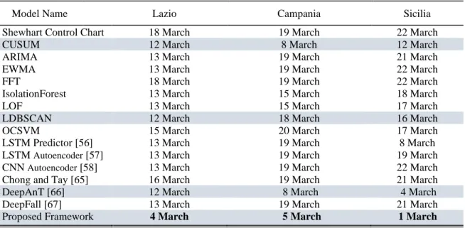
G. Performance Metric
In order to evaluate the performance of models, we measure the number of days until an anomaly is detected against the threshold level. In the context of this empirical study, an anomaly might mean that the COVID-19 pandemic might be moving out of control for the investigated region. According to European Centre for Disease Prevention and Control [95], the number of newly confirmed cases (or daily new positive cases) is one of the most accurate indicators of epidemic intensity. To compare the early COVID-19 outbreak detection performance, we compare the anomaly scores of models generated for the feature "new positive cases". For the prediction-based model, we use the one step prediction errors as anomaly scores. For the reconstruction-based models, we use the reconstruction errors as anomaly scores. OCSVM, IsolationForest, LOF and LDBSCAN models generate one anomaly score for each multivariate observation regardless of the feature monitored.
VI. RESULTS
A. FRAMEWORK PERFORMANCE
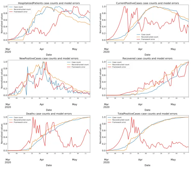
During the training process, the framework learns to reconstruct the selected features in each data point with the minimum possible error. In the case of anomalous events such as peaks of the COVID-19 pandemic, these reconstruction errors will get bigger, causing an alarm for the possible outbreak. The framework learns the normal data structure with the data from northern regions, which have gone through the pandemic earlier than other regions. To be able to detect the COVID-19 outbreak as early as possible, the framework must learn what the normal is when it is trained with highly contaminated data. As there is no label indicating anomalous events, the framework learns the distinctive patterns of abnormal events using the data from the nearest spatial neighbors.
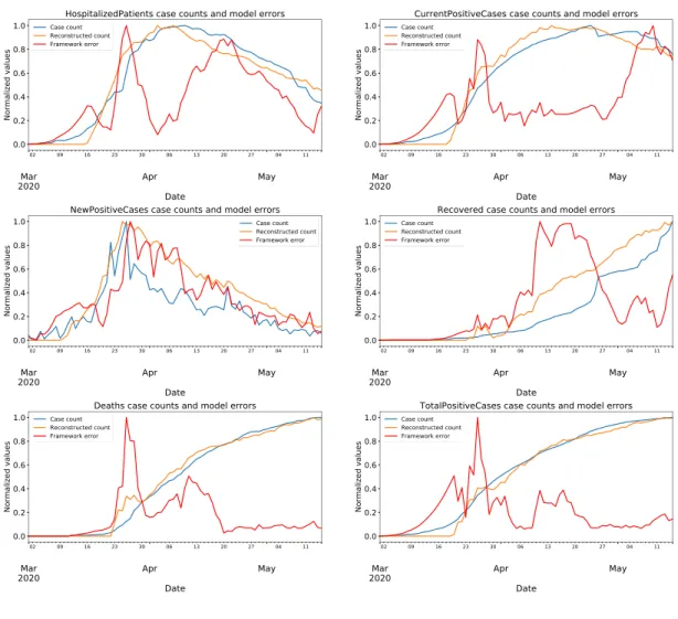
We train one unified deep learning model using the training set, which has a total of 684 spatio-temporal multivariate data points from 9 different regions. Then, we use the model to calculate the reconstruction errors of each 228 data points in the test set. As we set the window size to 7 days during the data preparation process and sliding step size to 1 day, we calculate the rolling window errors of each feature.
The reconstructed values and reconstruction errors for features "hospitalized patients, current positive cases, new positive cases, recovered cases, deaths, and total positive cases" on test data are plotted against the real case numbers in figures from 5 to 7. Test results for the region Lazio are given in Fig. 5; test results for the region Campania are given in Fig. 6; and test results for the region Sicilia are given in Fig. 7. In these figures, the real data are depicted in blue; the reconstructions are depicted in orange; and the reconstruction errors are depicted in red. All values are min-max normalized into the range of [0, 1] before plotting.