Search for Supersymmetry in pp Collisions at root s=13 TeV in the Single-Lepton Final State Using the Sum of Masses of Large-Radius Jets

EUROPEAN ORGANIZATION FOR NUCLEAR RESEARCH (CERN)

CERN-EP/2016-111 2018/03/05

CMS-SUS-15-007

Search for supersymmetry in pp collisions at

√

s

=

13 TeV

in the single-lepton final state using the sum of masses of

large-radius jets

The CMS Collaboration

Abstract

Results are reported from a search for supersymmetric particles in proton-proton col-lisions in the final state with a single, high transverse momentum lepton; multiple jets, including at least one b-tagged jet; and large missing transverse momentum. The data sample corresponds to an integrated luminosity of 2.3 fb−1 at√s = 13 TeV, recorded by the CMS experiment at the LHC. The search focuses on processes leading to high jet multiplicities, such as gluino pair production witheg→ttχe0₁. The quantity MJ, defined as the sum of the masses of the large-radius jets in the event, is used in conjunction with other kinematic variables to provide discrimination between signal and background and as a key part of the background estimation method. The ob-served event yields in the signal regions in data are consistent with those expected for standard model backgrounds, estimated from control regions in data. Exclusion limits are obtained for a simplified model corresponding to gluino pair production with three-body decays into top quarks and neutralinos. Gluinos with a mass be-low 1600 GeV are excluded at a 95% confidence level for scenarios with be-lowχe0₁mass, and neutralinos with a mass below 800 GeV are excluded for a gluino mass of about 1300 GeV. For models with two-body gluino decays producing on-shell top squarks, the excluded region is only weakly sensitive to the top squark mass.

Published in the Journal of High Energy Physics as doi:10.1007/JHEP08(2016)122.

c

2018 CERN for the benefit of the CMS Collaboration. CC-BY-3.0 license

∗_{See Appendix A for the list of collaboration members}

1

1

Introduction

Supersymmetry (SUSY) [1–8] is an extension of the standard model (SM) of particle physics that is motivated by several considerations, including the gauge hierarchy problem [9–14], the existence of astrophysical dark matter [15–17], and the possibility of gauge coupling constant unification at high energy [18–22]. In SUSY models, each SM particle has a corresponding supersymmetric partner (or partners) whose spin differs by one-half, such that fermions are mapped to bosons and vice versa. Gauge quantum numbers are preserved by this symmetry, and to preserve degrees of freedom, a SM spin-1/2 Dirac particle, such as the top quark, has two spin-0 partners, the top squarks. The SUSY partner of the (spin-1) gluon, the massless mediator of the strong interactions in the SM, is the spin-1/2 gluino. In R-parity–conserving models [23, 24], SUSY particles are produced in pairs, and the lightest supersymmetric particle (LSP) is stable. If the LSP is the lightest neutralino (χe0₁), an electrically neutral mixture of the SUSY partners of the neutral electroweak gauge and Higgs bosons, then it has weak interactions only and can in principle account for some or all of the dark matter.

The gauge hierarchy problem has become more urgent with the discovery of the Higgs bo-son [25–30]. Although the SM is conceptually complete, the Higgs bobo-son mass, together with the electroweak scale, is unstable against enormous corrections from loop processes, which pull the Higgs mass to the cutoff scale of the theory, for example, the Planck scale. This outcome can be avoided within the framework of the SM only with extreme fine tuning of the bare Higgs mass parameter, a situation that is regarded as unnatural, although not excluded. This prob-lem suggests that additional symmetries and associated degrees of freedom may be present that ameliorate these effects. So-called natural SUSY models [31–34], in which sufficiently light SUSY partners are present, are a major focus of current new physics searches at the CERN LHC. In natural models, several of the SUSY partners are constrained to be light [33]: both top squarks, etL and etR, which have the same electroweak couplings as the left- (L) and right- (R) handed top quarks, respectively; the bottom squark with L-handed couplings (ebL); the gluino (eg); and the Higgsinos (eh). While the gluino mass is not constrained by naturalness consid-erations as strongly as that of the lighter top squark mass eigenstate, et1, the cross section for gluino pair production is substantially larger than that for top squark pair production, for a given mass. As a consequence, the two types of searches can have comparable sensitivity to these models. Both types of searches are currently of intense interest, and CMS and ATLAS data taken at√s=8 TeV have provided significant constraints [35] on natural SUSY scenarios. This study uses the first LHC proton-proton collision data taken by the CMS experiment at √

s=13 TeV to search for gluino pair production. Searches targeting this process in the single-lepton final state using 8 TeV data have been performed by both ATLAS [36, 37] and CMS [38].

For m_eg = 1.5 TeV, somewhat above the highest gluino masses excluded at √s = 8 TeV, the

cross section for gluino pair production increases dramatically with center-of-mass energy,

from about 0.4 fb at √s = 8 TeV to about 14 fb at √s = 13 TeV [39]. In contrast, the cross

section for the dominant background, tt production, increases much more slowly, from about 248 pb at√s = 8 TeV to 816 pb at√s = 13 TeV [40]. As a consequence, the sensitivity of this

search can be significantly extended with respect to searches performed at √s = 8 TeV, even

though the 13 TeV data sample has an integrated luminosity of only 2.3 fb−1, roughly one-tenth of that acquired at 8 TeV.

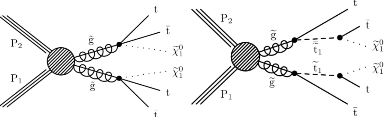
The search targets gluino pair production with eg → ttχe0₁, which arises fromeg → et1t, where the top squark is produced either on or off mass shell. The off-mass-shell scenario is shown in Fig. 1 (left) and is often designated T1tttt [41] in simplified model scenarios [42–44]. Results are also obtained for scenarios with on-shell top squark masses. This scenario is shown in

2 1 Introduction P1 P2 ˜g ˜ g ¯t t e χ01 e χ01 ¯t t

P

P

eg

eg

et

et

¯t

t

e

e

¯t

t

Figure 1: Gluino pair production and decay for the simplified models T1tttt (left) and T5tttt (right). In T1tttt, the gluino undergoes three-body decayeg → ttχe0₁ via a virtual intermediate top squark. In T5tttt, the gluino decays via the sequential two-body processeg→et1t, et1 →tχe0₁.

Because gluinos are Majorana particles, each one can decay to et1t and to the charge conjugate final state et1t.

Fig. 1 (right) and will be denoted by T5tttt. (For this scenario, the small contribution from the direct production of top squark pairs is also taken into account.) Regardless of whether the top squark is produced on or off mass shell, the final state is characterized by a large number of jets, four of which are b jets from top quark decays. Depending on the decay modes of the accompanying W bosons, a range of lepton multiplicities is possible; we focus here on the single-lepton final state, where the lepton is either an electron or a muon. Because the two neutralinos (χe0₁) are undetected, their production in SUSY events typically gives rise to a large amount of missing (unobserved) momentum, whose value in the direction transverse to the beam axis can be inferred from the momenta of the observed particles. The missing transverse momentum,~pmiss

T , is a key element of searches for R-parity-conserving SUSY, and

its magnitude is denoted by E_Tmiss.

A challenge in performing searches for SUSY particles is obtaining sufficient sensitivity to the signal, while at the same time understanding the background contribution from SM processes in a robust manner. This analysis is designed such that the background in the signal regions arises largely from a single process, dilepton tt production, in which both W bosons from t → bW+ decay leptonically, but only one lepton satisfies the criteria associated with

iden-tification, the minimum transverse momentum (pT) requirement, and isolation from other

en-ergy in the event. The search signature is characterized not only by the presence of high-pT jets and b-tagged jets, an isolated high-pT lepton, and large ETmiss, but also by additional kine-matic variables. Apart from resolution effects, the transverse mass of the lepton +~p_Tmisssystem, mT, is bounded above by mWfor events with a single leptonically decaying W, and this vari-able is very effective in suppressing the otherwise dominant single-lepton tt background. The quantity MJ, the scalar sum of the masses of large-radius jets, is used both to characterize the mass and energy scale of the event, providing discrimination between signal and background,

and as a key part of the background estimation. A property of MJ exploited in this analysis

is that, for the dominant background, this variable is nearly uncorrelated with mT. Because of the absence of correlation between MJand mT, the background shape at high mT, including the

signal region, can be measured to a very good approximation using a low-mT control sample.

The quantity MJwas first discussed in phenomenological studies, for example, in Refs. [45–47]. Similar variables have been used by ATLAS for SUSY searches in all-hadronic final states using

8 TeV data [48, 49]. We have presented studies of basic MJ properties and performance using

3

This paper is organized as follows. Section 2 gives a brief overview of the CMS detector. Sec-tion 3 discusses the simulated event samples used in the analysis. The event reconstrucSec-tion is discussed in Section 4, while Section 5 describes the trigger and event selection. Section 6 presents the methodology used to predict the SM background from the event yields in control regions in data. The associated systematic uncertainties are also discussed. The event yields observed in the signal regions are presented in Section 7. These yields are compared with back-ground predictions and used to obtain exclusion regions for the gluino pair production models shown in Fig. 1. Finally, Section 8 presents a summary of the methodology and the results.

2

Detector

The central feature of the CMS detector is a superconducting solenoid of 6 m internal diam-eter, providing a magnetic field of 3.8 T. Within the solenoid volume are the tracking and calorimeter systems. The tracking system, composed of silicon-pixel and silicon-strip detec-tors, measures charged particle trajectories within the pseudorapidity range|η| < 2.5, where η ≡ −ln[tan(θ/2)]and θ is the polar angle of the trajectory of the particle with respect to the

counterclockwise proton beam direction. A lead tungstate crystal electromagnetic calorimeter (ECAL), and a brass and scintillator hadron calorimeter (HCAL), each composed of a barrel

and two endcap sections, provide energy measurements up to |η| = 3. Forward

calorime-ters extend the pseudorapidity coverage provided by the barrel and endcap detectors up to |η| = 5. Muons are identified and measured within the range |η| < 2.4 by gas-ionization

de-tectors embedded in the steel magnetic flux-return yoke outside the solenoid. The detector is nearly hermetic, permitting the accurate measurement of~p_Tmiss. A more detailed description of the CMS detector, together with a definition of the coordinate system used and the relevant kinematic variables, is given in Ref. [51].

3

Simulated event samples

The analysis makes use of several simulated event samples for modeling the SM background and signal processes. While the background estimation in the analysis is performed largely from control samples in the data, simulated event samples provide correction factors, typically near unity. The equivalent integrated luminosity of the simulated event samples is at least six times that of the data, and at least 100 times that of the data in the case of tt and signal processes. The production of tt+jets, W+jets, Z+jets, and QCD multijet events is simulated with the Monte

Carlo (MC) generator MADGRAPH5 AMC@NLO 2.2.2 [52] in leading-order (LO) mode. Single

top quark events are modeled at next-to-leading order (NLO) with MADGRAPH5 AMC@NLO

for the s-channel andPOWHEGv2 [53, 54] for the t-channel and W-associated production. Addi-tional small backgrounds, such as tt production in association with bosons, diboson processes,

and t¯tt¯t are similarly produced at NLO with either MADGRAPH5 AMC@NLO orPOWHEG. All

events are generated using the NNPDF 3.0 [55] set of parton distribution functions (PDF).

Par-ton showering and fragmentation are performed with thePYTHIA8.205 [56] generator with the

underlying event model based on the CUETP8M1 tune detailed in Ref. [57]. The detector sim-ulation is performed with GEANT4 [58]. The cross sections used to scale simulated event yields are based on the highest order calculation available. For tt, in addition to using the next-to-next-to-leading order + next-to-next-to-next-to-leading logarithmic cross section calculation [40], the

modeling of the event kinematics is improved by reweighting the top quark pT spectrum to

match the data [59], keeping the overall normalization fixed.

4 4 Event reconstruction

that for the SM backgrounds, with the MADGRAPH5 AMC@NLO 2.2.2 generator in LO mode

using the NNPDF 3.0 PDF set and followed withPYTHIA 8.205 for showering and

fragmen-tation. The detector simulation is performed with the CMS fast simulation package [60] with scale factors applied to account for any differences with respect to the full simulation used for backgrounds. Event samples are generated for a representative set of model scenarios by scan-ning over the relevant mass ranges for theeg and eχ0₁, and the yields are normalized to the NLO

+ next-to-leading-logarithmic cross section [39, 61–64].

Throughout this paper, two T1tttt benchmark models are used to illustrate typical signal behav-ior. The T1tttt(1500,100) model, with masses m_eg = 1500 GeV and m_χe0

1 = 100 GeV, corresponds

to a scenario with a large mass splitting (referred to as non-compressed, or NC) between the gluino and the neutralino. This mass combination probes the sensitivity of the analysis to a low cross section (14 fb) process that has a hard E_Tmiss spectrum, which results in a relatively high signal efficiency. The T1tttt(1200,800) model, with masses m_eg= 1200 GeV and m_χe0

1 =800 GeV,

corresponds to a scenario with a small mass splitting (referred to as compressed, or C) between the gluino and the neutralino. Here the cross section is much higher (86 fb) because the gluino mass is lower than for the T1tttt(1500,100) model, but the sensitivity suffers from a low signal efficiency due to the soft Emiss

T spectrum.

Finally, to model the presence of additional proton-proton collisions from the same or adjacent beam crossing as the primary hard-scattering process (“pileup” interactions), the simulated events are overlaid with multiple minimum bias events, which are also generated with the PYTHIA 8.205 generator with the underlying event model based on the CUETP8M1 tune. The distribution of the number of overlaid minimum bias events is broad and peaks in the range 10–15.

4

Event reconstruction

The reconstruction of physics objects in an event proceeds from the candidate particles iden-tified by the particle-flow (PF) algorithm [65, 66], which uses information from the tracker, calorimeters, and muon systems to identify the candidates as charged or neutral hadrons, pho-tons, electrons, or muons. Charged particle tracks are required to originate from the event primary vertex (PV), defined as the reconstructed vertex, located within 24 cm (2 cm) of the center of the detector in the direction along (perpendicular to) the beam axis, that has the high-est value of p2_Tsummed over the associated charged particle tracks.

The charged PF candidates associated with the PV and the neutral PF candidates are clustered

into jets using the anti-kT algorithm [67] with distance parameter R = 0.4, as implemented

in the FASTJETpackage [68]. The estimated pileup contribution to the jet pT from neutral PF candidates is removed with a correction based on the area of the jet and the average energy density of the event [69]. The jet energy is calibrated using pT- and η-dependent corrections; the resulting calibrated jet is required to satisfy pT > 30 GeV and|η| ≤ 2.4. Each jet must also

meet loose identification requirements [70] to suppress, for example, calorimeter noise. Finally, jets that have PF constituents matched to an isolated lepton, as defined below, are removed from the jet collection.

A subset of the jets are “tagged” as originating from b quarks using the combined secondary vertex (CSV) algorithm [71, 72]. For the CSV medium working point chosen for this analysis, the signal efficiency for b jets in the range pT = 30 to 50 GeV is 60–67% (51–57%) in the barrel

(endcap), increasing with pT. Above pT ≈ 150 GeV the b tagging efficiency decreases. The

5

while the misidentification probability for light-flavor quarks or gluons is 1–2%.

Throughout this paper, quantities related to the number of jets (Njets) or to the number of b-tagged jets (N_b) are based only on small-R jets, not on the large-R jets discussed below.

Electrons are reconstructed by associating a charged particle track with an ECAL superclus-ter [73]. The resulting candidate electrons are required to have pT >20 GeV and|η| <2.5, and

to satisfy identification criteria designed to remove light-parton jets, photon conversions, and electrons from heavy flavor hadron decays. Muons are reconstructed by associating tracks in the muon system with those found in the silicon tracker [74]. Muon candidates are required to satisfy pT >20 GeV and|η| <2.4.

To preferentially select leptons that originate in the decay of W bosons, leptons are required to be isolated from other PF candidates. Isolation is quantified using an optimized version of the “mini-isolation” variable originally suggested in Ref. [75], in which the transverse energy of the particles within a cone in η-φ space surrounding the lepton momentum vector is computed using a cone size that scales as 1/p_T`, where p`_T is the transverse momentum of the lepton. In this analysis, mini-isolation, I_minirel , is defined as the transverse energy of particles in a cone of radius Rmini-iso _{around the lepton, divided by p}`

T. The transverse energy is computed as the

scalar sum of the pTvalues of the charged hadrons from the PV, neutral hadrons, and photons. The neutral hadron and photon contributions to this sum are corrected for pileup. The cone radius Rmini-isovaries with the p_T` according to

Rmini-iso=      0.2, p`_T ≤50 GeV

(10 GeV)/p`<sub>T</sub>, p`_T ∈ (50 GeV, 200 GeV)

0.05, p`_T ≥200 GeV.

(1)

The 1/p`_Tdependence is motivated by considering a two-body decay of a massive parent

par-ticle with mass M and large pT, for which the angular separation of the daughter particles is roughly∆Rdaughters≈2M/pT. The pT-dependent cone size reduces the rate of accidental over-laps between the lepton and jets in high-multiplicity or highly Lorentz-boosted events, partic-ularly overlaps between b jets and leptons originating from a boosted top quark. The cone re-mains large enough to contain b-hadron decay products for non-prompt leptons across a range of p`_Tvalues. Muons (electrons) must satisfy Irel

mini < 0.2 (0.1). The combined efficiency for the electron reconstruction and isolation requirements is about 50% at a p`<sub>T</sub>of 20 GeV, increasing to 65% at 50 GeV and reaching a plateau of 80% above 200 GeV. The combined reconstruction and isolation efficiencies for muons are about 70% at a p<sub>T</sub>` of 20 GeV, increasing to 80% at 50 GeV and reaching a plateau of 95% at 200 GeV.

We cluster R = 0.4 (“small-R”) jets and the isolated leptons into R = 1.2 (“large-R”) jets us-ing the anti-kT algorithm. The mass of the large-R jets retains angular information about the clustered objects, as well as their pTand multiplicity. Clustering small-R jets instead of PF can-didates incorporates the jet pileup corrections, thereby reducing the dependence of the mass on pileup. The variable MJis defined as the sum of all large-R jet masses:

MJ =

∑

Ji=large-R jets

m(Ji). (2)

The technique of clustering small-R jets into large-R jets has been used previously by ATLAS in, for example, Ref. [76]. Leptons are included in the large-R jets to include the full kinematics

of the event, and the choice R = 1.2 optimizes the background rejection power of MJ while

addi-6 5 Trigger and event selection [GeV] J M 0 200 400 600 800 1000 % events/(40 GeV) 1 − 10 1 10 2 10 Simulation CMSSimulation 13 TeV CMS 13 TeV (1500,100) 1 0 χ∼ t t → g ~ , g ~ g ~ , 1 true lepton t t , 2 true leptons t t < 10 GeV T ISR p [GeV] J M 0 200 400 600 800 1000 % events/(40 GeV) 1 − 10 1 10 2 10 Simulation CMSSimulation 13 TeV CMS 13 TeV (1500,100) 1 0 χ∼ t t → g ~ , g ~ g ~ , 1 true lepton t t , 2 true leptons t t > 100 GeV T ISR p

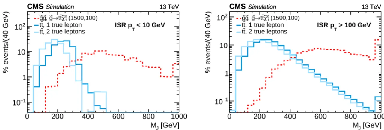
Figure 2: Distributions of MJ, normalized to the same area, from simulated event samples with a small ISR contribution (left) and a significant ISR contribution (right). These components are defined according to whether the pT of the tt system (or, in the case of signal events, that of theegeg system) is<10 GeV or>100 GeV, respectively. The T1tttt(NC) signal model (dashed red line), is described in Section 3; the first model parameter in parentheses corresponds to m_egand the second to m_χe0

1, both in units of GeV. The events satisfy the requirements E

miss

T > 200 GeV

and HT >500 GeV and have at least one reconstructed lepton.

tional discriminating power, while smaller parameters decrease the background rejection up to a factor of two for models with small mass splittings between the gluino and neutralino. For tt events with a small contribution from initial-state radiation (ISR), the MJdistribution has an approximate cutoff at twice the mass of the top quark, as shown in Fig. 2 (left). In contrast, the MJ distribution for signal events extends to larger values. The presence of a significant amount of ISR generates a high-MJtail in the tt background, as shown in Fig. 2 (right).

The missing transverse energy, Emiss_T , is given by the magnitude of~p_Tmiss, the negative vector sum of the transverse momenta of all PF candidates [65, 66]. Correspondence to the true un-detectable energy in the event is improved by replacing the contribution of the PF candidates associated with a jet by the calibrated four-momentum of that jet. To separate backgrounds characterized by the presence of a single W boson decaying leptonically but without any other source of missing energy, the lepton and the E_Tmissare combined to obtain the transverse mass, mT, defined as:

mT=

q

2p`<sub>T</sub>E<sub>T</sub>miss[1−cos(∆φ<sub>`,~p</sub>miss

T )], (3)

where∆φ_`,~pmiss

T is the difference between the azimuthal angles of the lepton momentum vector

and the missing momentum vector,~p_Tmiss. Finally, we define the quantity HT as the scalar sum of the transverse momenta of all the small-R jets passing the selection.

5

Trigger and event selection

The data sample used in this analysis was obtained with triggers that require HT > 350 GeV

and at least one electron or muon with pT > 15 GeV, where these variables are computed

with online (trigger-level) quantities and typically have somewhat poorer resolution than the corresponding offline variables. To ensure high trigger efficiency with respect to the offline definition of lepton isolation described in the previous section (mini-isolation), we designed these triggers with very loose lepton isolation requirements and fixed the isolation cone size to R=0.2. For events passing the offline selection, the total trigger efficiencies, measured in data control samples that are independently triggered, are found to be(95.1±1.1)% for the muon

7

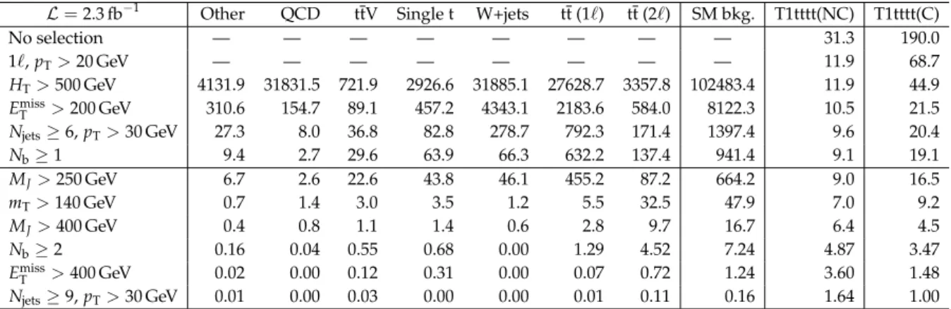
Table 1: Event yields obtained from simulated event samples, as the event selection criteria are applied. The category Other includes Drell–Yan, ttH(→bb), tttt, WZ, and WW. The yields for tt events in fully hadronic final states are included in the QCD multijet category. The category ttV includes ttW, ttZ, and ttγ. The benchmark signal models, T1tttt(NC) and T1tttt(C), are described in Section 3. The event selection requirements listed above the horizontal line in the middle of the table are defined as the baseline selection. The background estimates before the

HT requirement are not specified because some of the simulated event samples do not extend

to the low HT region. Given the size of the MC samples described in Section 3, rows with zero yield have statistical uncertainties of at most 0.16 events, and below 0.05 events in most cases.

L = 2.3 fb−1 _{Other QCD ttV Single t W+jets tt (1`) tt (2`) SM bkg. T1tttt(NC) T1tttt(C)}

No selection — — — — — — — — 31.3 190.0 1`, pT> 20 GeV — — — — — — — — 11.9 68.7 HT> 500 GeV 4131.9 31831.5 721.9 2926.6 31885.1 27628.7 3357.8 102483.4 11.9 44.9 Emiss T > 200 GeV 310.6 154.7 89.1 457.2 4343.1 2183.6 584.0 8122.3 10.5 21.5 Njets≥ 6, pT> 30 GeV 27.3 8.0 36.8 82.8 278.7 792.3 171.4 1397.4 9.6 20.4 Nb≥ 1 9.4 2.7 29.6 63.9 66.3 632.2 137.4 941.4 9.1 19.1 MJ> 250 GeV 6.7 2.6 22.6 43.8 46.1 455.2 87.2 664.2 9.0 16.5 mT> 140 GeV 0.7 1.4 3.0 3.5 1.2 5.5 32.5 47.9 7.0 9.2 MJ> 400 GeV 0.4 0.8 1.1 1.4 0.6 2.8 9.7 16.7 6.4 4.5 Nb≥ 2 0.16 0.04 0.55 0.68 0.00 1.29 4.52 7.24 4.87 3.47 Emiss T > 400 GeV 0.02 0.00 0.12 0.31 0.00 0.07 0.72 1.24 3.60 1.48 Njets≥ 9, pT> 30 GeV 0.01 0.00 0.03 0.00 0.00 0.01 0.11 0.16 1.64 1.00

channel and(94.1±1.2)% for the electron channel and are independent of the analysis vari-ables within the uncertainties. These efficiencies are applied to the simulation as a correction. The offline event selection is summarized in Table 1, which lists the event yields expected from simulation for both SM background processes and for the two benchmark T1tttt signal models. We select events with exactly one isolated charged lepton (an electron or a muon), HT > 500 GeV, ETmiss > 200 GeV, and at least six jets, at least one of which is b-tagged. After this set of requirements, referred in the following as the baseline selection, more than 80% of the remaining SM background arises from tt production. The contributions from events with a single top quark or a W boson in association with jets are each about 6–7%. The background from QCD multijet events after the baseline selection is negligible due to the combination of leptonic, Emiss

T , and Njetsrequirements.

After the baseline selection requirements are applied, events are binned in several other kine-matic variables, both to increase the signal sensitivity and to define control regions, as described in Section 6.1. To illustrate the effect of additional requirements, Table 1 lists the expected yields for examples of event selection requirements on MJ, mT, Njets, and Nb. The events satisfying the baseline selection are divided in the MJ-mT plane into a signal region, defined by the addi-tional requirements MJ > 400 GeV and mT > 140 GeV, and three control samples, bounded by MJ >250 GeV, that are used in the background estimation. Approximately 37% of signal T1tttt events are selected with the single-lepton requirement only. In non-compressed spectrum mod-els, for which m_egis significantly larger than m_χe0

1, more than half of the events passing the lepton

requirement lie in the signal region. For compressed spectrum models, where m_χe0

1 ≈meg−2mt,

the MJ, HT, and Emiss_T spectra become much softer and, as a result, only 5–10% of the single-lepton signal events are selected.

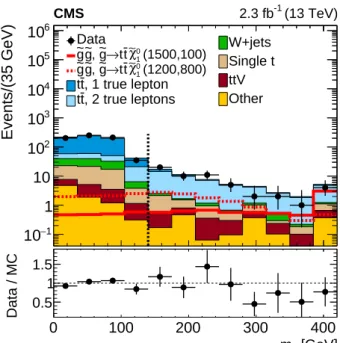
As shown in Fig. 3, backgrounds with a single W boson decaying leptonically are strongly

suppressed after the mT > 140 GeV requirement, so the total SM background in the signal

region is dominated by dilepton tt events. This dilepton background falls into two categories, which make roughly equal contributions. The first involves an identified electron or muon

8 6 Background estimation [GeV] T m Events/(35 GeV) 1 − 10 1 10 2 10 3 10 4 10 5 10 6 10 CMS 2.3 fb-1 (13 TeV) Data (1500,100) 1 0 χ∼ t t → g ~ , g ~ g ~ (1200,800) 1 0 χ∼ t t → g ~ , g ~ g ~ , 1 true lepton t t , 2 true leptons t t W+jets Single t ttV Other [GeV] T m 0 100 200 300 400 Data / MC 0.5 1 1.5

Figure 3: Distribution of mTin data and simulated event samples after the baseline selection is applied. The background contributions shown here are from simulation, and their total yield is normalized to the number of events observed in data. The signal distributions are normalized to the expected cross sections. The dashed vertical line indicates the mT > 140 GeV threshold that separates the signal regions from the control samples.

and a hadronically decaying τ from W decay. The second source involves two leptons, each of which is an electron or a muon. One of the leptons fails to satisfy the lepton selection criteria,

which include the pT and isolation requirements. This missed lepton can be produced either

directly or indirectly in W decay, where in the indirect case the lepton is the daughter of a τ.

6

Background estimation

6.1 Method

The prediction of the background yields in each of the signal bins takes advantage of the fact that the MJ and mT distributions of events with a significant amount of ISR are largely uncor-related. The correlation coefficients for the single-lepton and dilepton tt events in the MJ-mT plane after the baseline selection (as shown in Fig. 4) are small, in the range 0.03 to 0.05. The absence of a substantial correlation allows us to measure the MJdistribution of the background at low mTwith good statistical precision, and extrapolate it to high mT. The underlying expla-nation for this behavior is not immediately obvious, given that low-mTevents originate mainly from tt events where only one of the top quarks decays leptonically (1`tt), while the high-mT regions are dominated by dilepton tt events (2`tt). In particular, as shown in Fig. 2 (left), in the absence of significant ISR, the dileptonic tt events have a softer MJspectrum than single-lepton tt events, simply because the reconstructed mass of a leptonically decaying top quark does not include the undetected neutrino.

In events with substantial ISR, however, the contributions to MJfrom the accidental overlap of jets can dominate the contributions due to the intrinsic mass of the top quarks. This effect is illustrated in Fig. 5, which compares the Njetsand MJdistributions of single-lepton and dilepton tt events at high and low mT after the baseline selection is applied. Since we require at least

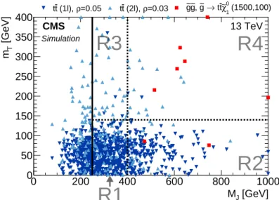
6.1 Method 9 [GeV] J M 0 200 400 600 800 1000 [GeV]_T m 0 50 100 150 200 250 300 350 400 =0.05 ρ (1l), t t tt (2l), ρ=0.03 0 (1500,100) 1 χ∼ t t → g ~ , g ~ g ~

R1

R2

R3

R4

Figure 4: Distribution of simulated single-lepton tt events (dark-blue triangles), dilepton tt events (light-blue inverted triangles), and T1tttt(1500,100) events (red squares) in the MJ-mT plane after the baseline selection. Each marker represents one expected event at 2.3 fb−1. Over-flow events are placed on the edge of the plot. The values of the correlation coefficients ρ for each background process are given in the legend. Region R4 is the nominal signal region, while R1, R2, and R3 serve as control regions. The small signal contributions in the control regions are taken into account in one of the global fits, as discussed in the text.

6 jets, single-lepton tt events must have at least 2 ISR jets and dilepton tt events must have at least 4. In this regime, the probability of additional ISR jets is similar for events with a given number of partons of similar momenta, and, as a result, the number of objects contributing to MJ (jets plus the reconstructed lepton) is comparable in 1` and 2` tt events. When these ISR jets overlap with the top quark decay products, the masses of the resulting large-R jets are dominated by the accidental overlap and, thus, the shapes of the MJdistribution of 1`and 2`tt events become more similar. This is the case for MJ >250 GeV, where Fig. 5 (right) shows that the distributions of the 1`and 2`tt backgrounds have nearly the same shape, and the low-mT to high-mTextrapolation is warranted.

We thus divide the MJ-mT plane into four regions, three control regions (CR) and one signal region (SR):

• Region R1 (CR): mT≤140 GeV, 250≤ MJ ≤400 GeV

• Region R2 (CR): mT≤140 GeV, MJ >400 GeV • Region R3 (CR): mT>140 GeV, 250≤ MJ ≤400 GeV • Region R4 (SR): mT >140 GeV, MJ >400 GeV. These regions are further subdivided into 10 bins of Emiss

T , Njets, and Nbto increase signal sen-sitivity:

• Six bins with 200 < Emiss_T ≤ 400 GeV: (6 ≤ Njets ≤ 8, Njets ≥ 9) × (Nb = 1, Nb = 2, Nb≥3)

• Four bins with Emiss_T >400 GeV:(6≤ Njets ≤8, Njets ≥9) × (Nb=1, Nb≥2),

where the multiplication indicates that the binning is two dimensional in Njets and Nb. Given that the main background processes have two or fewer b quarks, the total SM contribution to the Nb≥3 bins is very small and is driven by the b-tag fake rate. Signal events in the T1tttt and

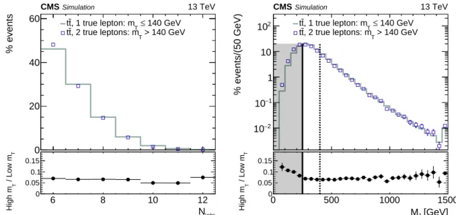
10 6 Background estimation jets N % events 0 20 40 60 Simulation CMS 13 TeV 140 GeV ≤ T , 1 true lepton: m t t > 140 GeV T , 2 true leptons: m t t jets N 6 8 10 12 T / Low m _T High m 0 0.05 0.1 0.15 [GeV] J M % events/(50 GeV) 2 − 10 1 − 10 1 10 2 10 Simulation CMS 13 TeV 140 GeV ≤ T , 1 true lepton: m t t > 140 GeV T , 2 true leptons: m t t [GeV] J M 0 500 1000 1500 T / Low m _T High m 0 0.05 0.1 0.15

Figure 5: Comparison of Njets and MJdistributions, normalized to the same area, in simulated tt events with two true leptons at high mT and one true lepton at low mT, after the baseline selection is applied. The shapes of these distributions are similar. These two contributions are the dominant backgrounds in their respective mT regions. The dashed vertical line on the right-hand plot indicates the MJ > 400 GeV threshold that separates the signal regions from

the control samples. The shaded region corresponding to MJ < 250 GeV is not used in the

background estimation.

T5tttt models are expected to populate primarily the bins with N_b ≥2, while bins with N_b=1 mainly serve to test the method in a background dominated region.

To obtain an estimate of the background rate in each of the signal bins, a modified version of an “ABCD” method is used. Here, the symbols A, B, C, and D refer to four regions in a two-dimensional space in the data, where one of the regions is dominated by signal and the other three by backgrounds. In a standard ABCD method, the background rate in the signal region is estimated from the yields in three control regions with the expression

µbkg_R4 = NR2NR3/NR1, (4)

where the labels on the regions correspond to those shown in Fig. 4. The background prediction is unbiased in the limit that the two variables that define the plane (in this case, MJ and mT) are uncorrelated. The effect of any residual correlation is corrected with factors κ that can be obtained from simulated event samples:

κ= N MC,bkg R4 /N MC,bkg R3 N_R2MC,bkg/N_R1MC,bkg. (5)

When the two ABCD variables are uncorrelated or nearly so, the κ factors are close to unity. This procedure ignores potential signal contamination in the control regions, which is ac-counted for by incorporating the constraints in Eqs. 4 and 5 into a fit that includes both signal and background components, as described in Section 6.2.

In principle, the background in the 10 signal bins could be estimated by applying this procedure in 10 independent planes. However, this procedure would incur large statistical uncertainties in some bins due to low numbers of events in R3. This problem is especially important in bins

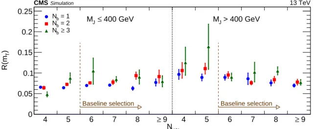
6.2 Implementation 11 4 5 6 7 8 ≥ 9 4 5 6 7 8 ≥ 9 )_T R(m 0 0.05 0.1 0.15 0.2 0.25 Simulation CMS 13 TeV

Baseline selection Baseline selection

= 1 b N = 2 b N 3 ≥ b N 400 GeV ≤ J M M_J > 400 GeV jets N

Figure 6: The ratio R(mT) of high-mT (R3 and R4) to low-mT (R1 and R2) event yields for the simulated SM background, as a function of Njets and Nb. The baseline selection requires Njets ≥6. The uncertainties shown are statistical only.

with a high number of jets, where the MJ spectrum shifts to higher values and the number of

background events expected in R4 can exceed the background in R3.

To alleviate this problem, we exploit the fact that, after the baseline selection, the background is dominated by just one source (tt events), and the shapes of the Njets distributions are nearly identical for the single-lepton and dilepton components (due to the large amounts of ISR). As a result, the mT distribution is approximately independent of Njets and Nb. We study this behavior with the ratio of the number of events at high to low mT:

R(mT) ≡

N(mT >140 GeV) N(mT ≤140 GeV)

. (6)

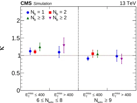
Because, as seen in Fig. 6, the values of R(mT) do not vary substantially across Njets and Nb bins, the predicted value of R(mT)is not sensitive to the modeling of the distributions of those quantities. We exploit this result by integrating the yields of the low-MJ regions (R1 and R3) over the Njets and Nbbins for each EmissT bin. This procedure increases the statistical power of the ABCD method but also introduces a correlation among the predictions (Eq. 4) for the Njets and Nb bins associated with a given EmissT bin. Figure 7 shows the κ factors for the 10 signal bins after summing over Njets and Nbin R1 and R3. In all cases, their values are close to unity.

6.2 Implementation

The method outlined in Section 6.1 is implemented with a likelihood function that incorpo-rates the statistical and systematic uncertainties in κ, accounts for correlations arising from the common R1 and R3 yields, and corrects for signal contamination in the control regions.

The SM background contribution for each region is described as follows. We define µbkg_Ri as

the estimated (Poisson) mean background in each region Ri, with i = 1, 2, 3, 4. Then, in an

ABCD background calculation, these four rates can be expressed in terms of three floating fit parameters µ, R(mT), and R(MJ), and the correlation correction factor κ, as

µbkg_R1 =µ, µbkg_R2 =µ R(MJ),

µbkg_R3 =µ R(mT), µbkg_R4 =κ µ R(MJ)R(mT).

12 6 Background estimation

400 ≤

miss T

E Emiss_T > 400 Emiss_T ≤ 400 Emiss_T > 400

κ

0

0.5

1

1.5

2

Figure 7: Values of the double-ratio κ in each of the 10 signal bins, calculated using the simu-lated SM background. The κ factors are close to unity, indicating the small correlation between MJ and mT. The uncertainties shown are statistical only.

Here, µ is the background rate fit parameter for R1, R(MJ)is the ratio of the R2 to R1 rates, and R(mT)is the ratio of the R3 to R1 rates. The quantity κ is given by Eq. 5 after replacing the yields N_RiMC,bkgby the background rate fit parameters µMC,bkg_Ri .

Similarly, we define N_Ridata as the observed data yield in each region, µMC,sig_Ri as the expected signal rate in each region, and r as the parameter quantifying the signal strength relative to the expected yield across all analysis regions. We can then write the likelihood function as

L = Ldata_ABCDLMC_κ LMC_sig , (8)

Ldata_ABCD = 4

∏

∏

Poisson(N_Ri,kdata|µbkg_Ri,k+r µMC,sig_Ri,k ), (9)

LMC_κ = 4

∏

∏

Poisson(N_Ri,kMC,bkg|µMC,bkg_Ri,k ), (10)

LMC sig = 4

∏

∏

Poisson(N_Ri,kMC,sig|µMC,sig_Ri,k ). (11)

The indices k run over each of the E_Tmiss, Njets, and Nbbins defined in the previous section; these indices were suppressed in Eq. 7 for simplicity. Given the integration over Njetsand Nbat low MJ, Nbins(R1) =Nbins(R3) =2, while Nbins(R2) =Nbins(R4) =10.

In Eq. 8, Ldata

ABCD accounts for the statistical uncertainty in the observed data yield in the four

ABCD regions, and LMC

κ and LMCsig account for the uncertainty in the computation of the κ

correction factor and signal shape, respectively, due to the finite size of the MC samples. The systematic uncertainties in κ and the signal efficiency are described in the following sec-tions. These effects are incorporated in the likelihood function as log-normal constraints with a

6.3 Systematic uncertainties 13

nuisance parameter for each uncorrelated source of uncertainty. These terms are not explicitly shown in the likelihood function above for simplicity.

The likelihood function defined in Eqs. 8–11 is employed in two separate types of fits that pro-vide complementary but compatible background estimates based on an ABCD model. The first type of fit, which we call the predictive fit, allows us to more easily establish the agreement of the background predictions and the observations in the null (i.e., the background-only) hypothe-sis. We do this by excluding the observations in the signal regions in the likelihood (that is, by truncating the first product in Eq. 9 at i = 3) and fixing the signal strength r to 0. This proce-dure leaves as many unknowns as constraints: three data floating parameters (µ, R(MJ), and R(mT)) and three observations (N_Ri,kdatawith i = 1, 2, 3) for each ABCD plane. In the likelihood function there are additional floating parameters associated with MC quantities, which have small uncertainties. As a result, the estimated background rates in regions R1, R2, and R3 con-verge to the observed values in those bins, and we obtain predictions for the signal regions that do not depend on the observed N_R4data. The predictive fit thus converges to the standard ABCD method, and the likelihood machinery becomes just a convenient way to solve the system of equations and propagate the various uncertainties.

Additionally, we implement a global fit which, by making use of the observations in the signal regions, can provide an estimate of the signal strength r, while allowing for signal events to populate the control regions. This is achieved by including all four observations, N_Ri,kdata with i = 1, 2, 3, 4, in the likelihood function. Since there are four observations and three float-ing background parameters in each ABCD plane, there are enough constraints for the signal strength also to be determined in the fit.

6.3 Systematic uncertainties

This section describes the systematic uncertainties in the background prediction, which are incorporated into the analysis as an uncertainty in the κ correction. Because the dominant

background arises from 2`tt events, we use a control sample with two reconstructed leptons

to validate our background estimation procedure and to quantify the associated uncertainty. The resulting uncertainty is augmented with simulation-based studies of effects that are not covered by this dilepton test. Table 2 summarizes all of the uncertainties in the background prediction.

The ability of the ABCD method to predict the 2`tt background is studied using a modified

ABCD plane, in which the high-mT regions, R3 and R4, are replaced with regions D3 and D4,

which have two reconstructed leptons. These regions have low and high MJ, respectively, just as R3 and R4. The events in D3 and D4 pass the same selection as those in R3 and R4, except for the following changes: Njets bin boundaries are lowered by one to keep the number of large-R jet constituents the same as in the single-lepton samples; the mT requirement is not applied; and events with Nb=0 are included to increase the size of the event sample, while events with Nb ≥ 3 are excluded to avoid signal contamination. We perform this test only for low EmissT to further avoid the potentially large signal contribution in the high-Emiss_T region. The low-MJ regions (R1 and D3) are integrated over Njets, while the high-MJregions (R2 and D4) are binned in low and high Njets. The predictive fit is then used to predict the D4 event yields for both Njets bins. We predict 11.0±2.3 (1.5±0.5) events for the low (high) Njetsbin, and we observe 12 (2) events. Given the good agreement between prediction and observation, the statistical precision of the test is taken as a systematic uncertainty in κ. These uncertainties are 37% and 88% for the low- and high-Njetsregions, respectively.

14 7 Results and interpretation

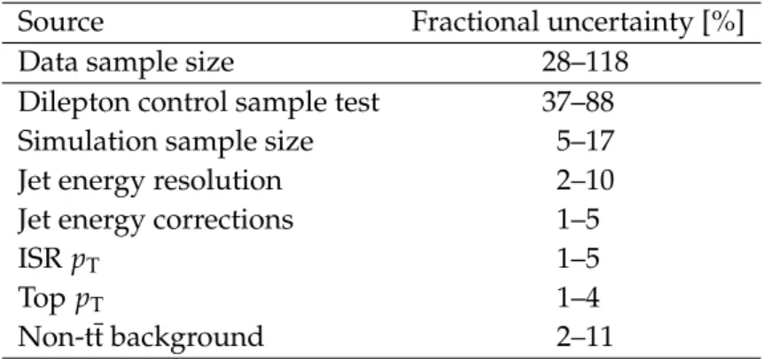
Table 2: Summary of uncertainties in the background predictions. All entries in the table ex-cept for data sample size correspond to a relative uncertainty on κ. The ranges indicate the spread of each uncertainty across the signal bins. Uncertainties from a particular source are treated as fully correlated across bins, while uncertainties from different sources are treated as uncorrelated.

Source Fractional uncertainty [%]

Data sample size 28–118

Dilepton control sample test 37–88

Simulation sample size 5–17

Jet energy resolution 2–10

Jet energy corrections 1–5

ISR pT 1–5

Top pT 1–4

Non-tt background 2–11

and R4, we perform studies on potential additional sources of systematic uncertainty in the simulation. We find that the main source of 1` tt events in the high-mT region is jet energy mismeasurement. We study the impact of mismodeling the size of this contribution by smear-ing the jet energies by an additional 50% with respect to the jet energy resolution measured in data [70] and calculating the corresponding shift in κ. To ensure that there are no further significant differences between the MJshapes of events reconstructed with one or two leptons, we also calculate the shift in κ due to jet energy corrections, potential ISR pT and top quark

pT mismodeling, as well as the amount of non-tt background. Even though each of these can

alone have a significant effect on the MJ shape, the κ factor, as a double ratio, remains largely unaffected (Table 2). Including these uncertainties in the likelihood fit produces a negligible contribution to the total uncertainty.

7

Results and interpretation

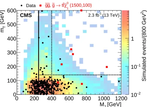
Figure 8 shows the two-dimensional distribution of the data in the mT-MJplane after the base-line selection, but with the additional requirement Nb ≥ 2. The baseline requirements include E_Tmiss > 200 GeV and Njets ≥ 6, but no further event selection is applied. For comparison, the plot also shows the expected total SM background based on simulation, as well as a particular sample of the expected signal distribution. The overall distribution of events in data is consis-tent with the background expectation, where the majority of events are concentrated at low mT and MJ. In R4, the nominal signal region, we observe only two events in data, while, as shown in Table 3, the predicted SM background is about 5 events. The T1tttt(1500,100) (NC) model would be expected to contribute 5 additional events to R4.

The validity of the central assumption of the background estimation method can be checked in

the nearly signal-free Nb = 1 region by comparing the MJ shapes observed in the high- and

low-mTregions in data. Figure 9 (left) shows the MJ shapes in the Nb =1 sample, integrating over the Njets and EmissT bins. The low mT data have been normalized to the overall yields in the corresponding high-mT data. The shapes of the MJ distributions for the high- and low-mT regions are consistent. Figure 9 (right) shows that the corresponding distributions in the Nb≥2 sample are also consistent, as expected in the absence of signal.

Table 3 summarizes the observed event yields, the fitted backgrounds, and the expected signal yields for the two T1tttt benchmark model points. Two background estimates are given: the

15

)

2

Simulated events/(800 GeV

2 −

10

10

1

[GeV]

M

0

200

400

600

800

1000 1200

[GeV]

m

0

100

200

300

400

500

600

Figure 8: Two-dimensional distributions for data and simulated event samples in the vari-ables mTand MJ in the Nb ≥ 2 region after the baseline selection. The distributions integrate over the Njets and Emiss_T bins. The black dots are the data; the colored histogram is the total simulated background, normalized to the data; and the red dots are a particular signal sam-ple drawn from the expected distribution for gluino pair production in the T1tttt model with m_eg=1500 GeV and m_χe0

1 =100 GeV for 2.3 fb

−1_{. Overflow events are shown on the edges of the} plot. The definitions of the signal and control regions are the same as those shown in Fig. 4.

[GeV] J M 200 400 600 Events/(75 GeV) 0 5 10 15 20 CMS 2.3 fb-1 (13 TeV) > 140 GeV T Data, m 140 GeV ≤ T Data, m (1500,100) 1 0 χ∼ t t → g ~ , g ~ g ~ (1200,800) 1 0 χ∼ t t → g ~ , g ~ g ~ = 1 b N [GeV] J M 200 400 600 Events/(75 GeV) 0 5 10 15 CMS 2.3 fb-1 (13 TeV) > 140 GeV T Data, m 140 GeV ≤ T Data, m (1500,100) 1 0 χ∼ t t → g ~ , g ~ g ~ (1200,800) 1 0 χ∼ t t → g ~ , g ~ g ~ 2 ≥ b N

Figure 9: Comparison of the MJ distributions for low- and high-mT in data with Nb = 1 (left) and Nb≥2 (right) after the baseline selection. The expected MJdistributions of the two bench-mark T1tttt scenarios for mT >140 GeV are overlaid. The distributions integrate over the Njets and Emiss

T bins. The low-mTdistribution is normalized to the number of events in the high-mT

region. The dashed vertical lines indicate the MJ >400 GeV threshold that separates the signal regions from the control samples.

16 7 Results and interpretation

predictive fit (PF), which uses only the yields in regions R1, R2, and R3, and the global fit (GF), which also incorporates region R4, as described in Section 6. In both versions of the fit, the signal strength r is fixed to zero, giving results that are model independent. (When setting limits on individual models, we allow r to float, as discussed below.) The rows labeled R4 give the results for each of the ten signal regions, as well as the corresponding κ factors.

In the absence of signal, the predictive fit and the version of the global fit performed under the null hypothesis, r = 0, should be consistent with each other. However, because the global fit incorporates more information, specifically the yields in R4, this fit has a smaller uncertainty.

The regions with Nb = 1 have small expected contributions from signal. Summing over all

four such signal regions (R4), the number of estimated background events from the PF and

GF are 6.1±2.2 and 5.5±1.3, respectively, compared with 8 events observed in data. The

consistency between the two predictions and between the predicted and observed yields in the R4 regions with Nb = 1, where the signal contribution is expected to be small, serves as a further check on the background estimation method. Summing the yields over the six signal

bins with Nb ≥ 2, the number of estimated background events from PF and GF is 5.6±1.6

and 4.9±1.0, respectively. In data, we observe 2 events, lower than, but consistent with the background-only hypothesis.

Given the absence of any significant excess, the results are interpreted first as exclusion limits on the production cross section for T1tttt model points as a function of m_egand m_χe0

1. Table 4

shows the ranges for the systematic uncertainties associated with predictions for the expected signal yields, including those on the signal efficiency. The largest uncertainties arise from the jet energy corrections and from the modeling of ISR. These uncertainties are generally in the

range 10–20% but can increase to ∼30% as the mass splitting between the gluino and LSP

decreases [77]. The uncertainty associated with the renormalization and factorization scales is determined by varying the scales independently up and down by a factor of two; these are applied only as an uncertainty in the signal shape, i.e., the cross section is held constant. The uncertainty associated with the b tagging efficiency is in the range 1–15%. Uncertainties due to pileup, luminosity [78], lepton selection, and trigger efficiency are found to be≤ 5%. Uncertainties for each particular source are treated as fully correlated across bins.

A 95% confidence level (CL) upper limit on the production cross section is estimated using the modified frequentist CLSmethod [79–81], with a one-sided profile likelihood ratio test statistic. For this test, we perform the global fit under the background-only and background-plus-signal (r floating) hypotheses. The statistical uncertainties from data counts in the control regions are modeled by the Poisson terms in Eq. 9. All systematic uncertainties are multiplicative and are treated as log-normal distributions. Exclusion limits are also estimated for±1σ variations on the production cross section based on the NLO+NLL calculation [39].

Figure 10 shows the corresponding excluded region at a 95% CL for the T1tttt model in the m_eg−m_χe0

1plane. At lowχe

0

1mass we exclude gluinos with masses of up to 1600 GeV. The highest

limit on theχe0₁mass is 800 GeV, attained for m_egof approximately 1300 GeV. The observed limits are within the 1σ uncertainty in the expected limits. The central value is slightly higher because the observed event yield is less than the SM background prediction, as shown in Table 3. In the context of natural SUSY models, it is important to extend the interpretation to scenarios in which the top squark is lighter than the gluino. Rather than considering a large set of models with independently varying top squark masses, we consider the extreme case in which the top squark has approximately the smallest mass consistent with two-body decay, m_et1 ≈ mt+mχ_e0₁, for a range of gluino and neutralino masses. The decay kinematics for such extreme,

com-17

Table 3: Observed and predicted event yields for the signal regions (R4) and background re-gions (R1–R3) in data (2.3 fb−1). Expected yields for the two SUSY T1tttt benchmark scenarios are also given. The results from two types of fits are reported: the predictive fit (PF) and the version of the global fit (GF) performed under the assumption of the null hypothesis (r = 0). The predictive fit uses the observed yields in regions R1, R2, and R3 only and is effectively just a propagation of uncertainties. The global fit uses all four regions. The values of κ obtained from the simulation fit are also listed. The first uncertainty in κ is statistical, while the second corresponds to the total systematic uncertainty. The benchmark signal models, T1tttt(NC) and T1tttt(C), are described in Section 3.

Region: bin κ T1tttt(NC) T1tttt(C) Fitted µbkg(PF) Fitted µbkg(GF) Obs.

200 < Emiss T ≤ 400 GeV R1: all Njets, Nb — 0.1 3.2 336.0 ± 18.3 335.3 ± 18.2 336 R2: 6 ≤ Njets≤ 8, Nb= 1 — 0.1 0.2 47.1 ± 6.9 49.5 ± 6.9 47 R2: Njets≥ 9, Nb= 1 — 0.1 0.3 7.0 ± 2.6 7.5 ± 2.7 7 R2: 6 ≤ Njets≤ 8, Nb= 2 — 0.1 0.3 42.0 ± 6.5 41.1 ± 6.2 42 R2: Njets≥ 9, Nb= 2 — 0.1 0.5 7.0 ± 2.6 6.6 ± 2.5 7 R2: 6 ≤ Njets≤ 8, Nb≥ 3 — 0.1 0.2 12.0 ± 3.5 11.1 ± 3.2 12 R2: Njets≥ 9, Nb≥ 3 — 0.2 0.6 1.0 ± 1.0 0.9 ± 0.9 1 R3: all Njets, Nb — 0.2 3.8 21.0 ± 4.6 21.6 ± 4.2 21 R4: 6 ≤ Njets≤ 8, Nb= 1 1.12 ± 0.09 ± 0.43 0.2 0.2 3.3 ± 1.4 3.6 ± 1.0 6 R4: Njets≥ 9, Nb= 1 0.91 ± 0.06 ± 0.81 0.2 0.4 0.4 ± 0.3 0.4 ± 0.2 1 R4: 6 ≤ Njets≤ 8, Nb= 2 1.11 ± 0.06 ± 0.42 0.3 0.4 2.9 ± 1.2 2.9 ± 0.8 2 R4: Njets≥ 9, Nb= 2 1.05 ± 0.11 ± 0.94 0.3 0.6 0.5 ± 0.3 0.4 ± 0.2 0 R4: 6 ≤ Njets≤ 8, Nb≥ 3 1.25 ± 0.11 ± 0.47 0.3 0.3 0.9 ± 0.4 0.9 ± 0.3 0 R4: Njets≥ 9, Nb≥ 3 1.05 ± 0.10 ± 0.93 0.3 0.7 0.1 ± 0.1 0.1 ± 0.1 0 Emiss T > 400 GeV R1: all Njets, Nb — 0.1 0.5 16.0 ± 4.0 17.1 ± 4.0 16 R2: 6 ≤ Njets≤ 8, Nb= 1 — 0.2 0.1 8.0 ± 2.8 6.8 ± 2.5 8 R2: Njets≥ 9, Nb= 1 — 0.1 0.2 1.0 ± 1.0 1.7 ± 1.2 1 R2: 6 ≤ Njets≤ 8, Nb≥ 2 — 0.5 0.3 3.0 ± 1.7 2.5 ± 1.4 3 R2: Njets≥ 9, Nb≥ 2 — 0.4 0.6 1.0 ± 1.0 0.9 ± 0.9 1 R3: all Njets, Nb — 0.4 0.9 4.0 ± 2.0 2.9 ± 1.4 4 R4: 6 ≤ Njets≤ 8, Nb= 1 1.09 ± 0.16 ± 0.42 0.7 0.2 2.2 ± 1.7 1.2 ± 0.7 0 R4: Njets≥ 9, Nb= 1 0.98 ± 0.16 ± 0.87 0.4 0.3 0.2 ± 0.3 0.3 ± 0.2 1 R4: 6 ≤ Njets≤ 8, Nb≥ 2 1.29 ± 0.22 ± 0.50 1.9 0.5 1.0 ± 0.8 0.5 ± 0.4 0 R4: Njets≥ 9, Nb≥ 2 0.90 ± 0.14 ± 0.80 1.6 1.0 0.2 ± 0.3 0.1 ± 0.1 0

18 8 Summary

Table 4: Typical values of the signal-related systematic uncertainties. Uncertainties due to a particular source are treated as fully correlated between bins, while uncertainties due to differ-ent sources are treated as uncorrelated.

Source Fractional uncertainty [%]

Lepton efficiency 1–5

Trigger efficiency 1

b tagging efficiency 1–15

Jet energy corrections 1–30

Renormalization and factorization scales 1–5

Initial state radiation 1–35

Pileup 5

Integrated luminosity 3

pressed mass spectrum models correspond to the lowest signal efficiency for given values of m_eg and m_χe0

1, because the top quark and theχe

0

1 are produced at rest in the top squark frame.

As a consequence, the excluded signal cross section for fixed values of m_egand m_χe0

1 and with

m_eg>m_et

1 ≥mt+mχe0₁ is minimized around this extreme model point. For physical consistency, the signal model used in this study, both in the fit procedure and in the theoretical cross section used to obtain mass limits, includes not only gluino-pair production, but also direct et1et1 pro-duction. However, the effect of the direct top squark contribution on the results is small,.2% for m_χe0

1 >400 GeV and up to 20% for low values of mχe01.

Figure 11 shows the excluded region in the m_eg-m_χe0

1 plane for this combined model with both

gluino-mediated top squark production and direct top squark pair production. The top squark mass is assumed to be 175 GeV above that of the neutralino. For most of the excluded region, the boundary is close to that obtained for the T1tttt model, showing that there is only a weak sensitivity to the value of the top squark mass. The uncertainty on the boundary of the ex-cluded region for the T5tttt model is similar to that shown for the T1tttt model in Fig. 10. For m_χe0

1 >150 GeV, the excluded value of megis typically within 60 GeV of that excluded for T1tttt.

Models that have low values of m_χe0

1 show a reduced sensitivity because the neutralino carries

very little momentum, reducing the value of mT. In this kinematic region, the sensitivity to the signal is dominated by the events that have at least two leptonic W boson decays, which produce additional Emiss_T , as well as a tail in the mTdistribution. Although such dilepton events are nominally excluded in the analysis, a significant number of these signal events escape the dilepton veto. These events include both W decays to τ leptons that decay hadronically, and W decays to electrons or muons that are below kinematic thresholds or are outside of the detector acceptance.

8

Summary

Using a sample of proton-proton collisions at √s = 13 TeV with an integrated luminosity of

2.3 fb−1, a search for supersymmetry is performed in the final state with a single lepton, b-tagged jets, and large missing transverse momentum. The search focuses on final states result-ing from the pair production of gluinos, which subsequently decay via eg → ttχe0₁, leading to high jet multiplicities.

A key feature of the analysis is the use of the variable MJ, the sum of the masses of large-R jets, which are formed by clustering anti-kT R=0.4 jets and leptons. Used in conjunction with

19

[GeV]

m

[GeV]

m

(13 TeV)

2.3 fb

CMS

95% CL upper limit on cross section [pb]

Figure 10: Interpretation of results in the T1tttt model. The colored regions show the upper limits (95% CL) on the production cross section for pp → _{egeg, eg} → ttχe0₁ in the m_eg-m_χe0

1 plane.

The curves show the expected and observed limits on the corresponding SUSY particle masses obtained by comparing the excluded cross section with theoretical cross sections.

20 8 Summary

[GeV]

m

[GeV]

m

CMS

Figure 11: Excluded region (95% CL), shown in blue, in the m_eg-m_χe0

1 plane for a model

com-bining T5tttt, gluino pair production, followed by gluino decay to an on-shell top squark, to-gether with a model for direct top squark pair production. The top squarks decay via the two-body process et→tχe0₁. The neutralino and top squark masses are related by the constraint m_et1 =m_χe0

1 +175 GeV. For comparison, the excluded region (95% CL) from Fig. 10 for the T1tttt

model, which has three-body gluino decay, is shown in red. The small difference between the two boundary curves shows that the limits for the scenarios with two-body gluino decay have only a weak dependence on the top squark mass.

21

the variable mT, the transverse mass of the system consisting of the lepton and the missing

transverse momentum vector, MJ provides a powerful background estimation method that is

well suited to this high jet multiplicity search.

After the baseline selection is applied, signal (R4) and control regions (R1, R2, and R3) are de-fined in the MJ-mTplane, which are further divided into bins of EmissT , Njets, and Nbto provide additional sensitivity. In regions R3 and R4, the requirement mT > 140 GeV provides strong suppression of the single-lepton tt background, so that dilepton tt events dominate over all other background sources. For these dilepton events to enter a signal region, however, they must contain a substantial amount of initial-state radiation (ISR). For this extreme range of ISR jet momentum and multiplicity, the single-lepton and dilepton tt events have very similar

kinematic properties. The variables MJ and mT are nearly uncorrelated, even though

differ-ent processes dominate the low- and high-mT regions. As a consequence, the low-mT regions

(R1 and R2) can be used to measure the background shape for the MJdistribution at high mT. A correction factor, near unity, is taken from simulation and is used to account for a possible correlation between MJand mT.

The observed event yields in the signal regions are consistent with the predictions for the SM background contributions, and exclusion limits are set on the gluino pair production cross sections in the m_eg-m_χe0

1 plane, as described by the simplified models T1tttt and T5tttt, where the

latter is augmented with a model of direct top squark pair production for consistency. In the T1tttt model, gluinos decay via the three-body processeg →ttχe0₁, which proceeds via a virtual top squark in the intermediate state. Under the assumption of a 100% branching fraction to this final state, the cross section limit for each model point is compared with the theoretical cross section to determine the excluded particle masses. Gluinos with a mass below 1600 GeV are excluded at a 95% CL for scenarios with lowχe0₁mass, and neutralinos with a mass below 800 GeV are excluded for a gluino mass of about 1300 GeV. In the T5tttt model, the top squark is lighter than the gluino, which therefore decays via a two-body process. The boundary of the excluded region in the m_eg-m_χe0

1 plane for T5tttt is found to be only weakly sensitive to the top

squark mass. These results significantly extend the sensitivity of single-lepton searches based on data at√s=8 TeV.

Acknowledgments

We congratulate our colleagues in the CERN accelerator departments for the excellent perfor-mance of the LHC and thank the technical and administrative staffs at CERN and at other CMS institutes for their contributions to the success of the CMS effort. In addition, we grate-fully acknowledge the computing centers and personnel of the Worldwide LHC Computing Grid for delivering so effectively the computing infrastructure essential to our analyses. Fi-nally, we acknowledge the enduring support for the construction and operation of the LHC and the CMS detector provided by the following funding agencies: the Austrian Federal Min-istry of Science, Research and Economy and the Austrian Science Fund; the Belgian Fonds de la Recherche Scientifique, and Fonds voor Wetenschappelijk Onderzoek; the Brazilian Fund-ing Agencies (CNPq, CAPES, FAPERJ, and FAPESP); the Bulgarian Ministry of Education and Science; CERN; the Chinese Academy of Sciences, Ministry of Science and Technology, and Na-tional Natural Science Foundation of China; the Colombian Funding Agency (COLCIENCIAS); the Croatian Ministry of Science, Education and Sport, and the Croatian Science Foundation; the Research Promotion Foundation, Cyprus; the Ministry of Education and Research, Esto-nian Research Council via IUT23-4 and IUT23-6 and European Regional Development Fund, Estonia; the Academy of Finland, Finnish Ministry of Education and Culture, and Helsinki

22 References

Institute of Physics; the Institut National de Physique Nucl´eaire et de Physique des Partic-ules / CNRS, and Commissariat `a l’ ´Energie Atomique et aux ´Energies Alternatives / CEA, France; the Bundesministerium f ¨ur Bildung und Forschung, Deutsche Forschungsgemeinschaft, and Helmholtz-Gemeinschaft Deutscher Forschungszentren, Germany; the General Secretariat for Research and Technology, Greece; the National Scientific Research Foundation, and Na-tional Innovation Office, Hungary; the Department of Atomic Energy and the Department of Science and Technology, India; the Institute for Studies in Theoretical Physics and Mathematics, Iran; the Science Foundation, Ireland; the Istituto Nazionale di Fisica Nucleare, Italy; the Min-istry of Science, ICT and Future Planning, and National Research Foundation (NRF), Repub-lic of Korea; the Lithuanian Academy of Sciences; the Ministry of Education, and University of Malaya (Malaysia); the Mexican Funding Agencies (BUAP, CINVESTAV, CONACYT, LNS, SEP, and UASLP-FAI); the Ministry of Business, Innovation and Employment, New Zealand; the Pakistan Atomic Energy Commission; the Ministry of Science and Higher Education and the National Science Centre, Poland; the Fundac¸˜ao para a Ciˆencia e a Tecnologia, Portugal; JINR, Dubna; the Ministry of Education and Science of the Russian Federation, the Federal Agency of Atomic Energy of the Russian Federation, Russian Academy of Sciences, and the Russian Foundation for Basic Research; the Ministry of Education, Science and Technologi-cal Development of Serbia; the Secretar´ıa de Estado de Investigaci ´on, Desarrollo e Innovaci ´on and Programa Consolider-Ingenio 2010, Spain; the Swiss Funding Agencies (ETH Board, ETH Zurich, PSI, SNF, UniZH, Canton Zurich, and SER); the Ministry of Science and Technology, Taipei; the Thailand Center of Excellence in Physics, the Institute for the Promotion of Teach-ing Science and Technology of Thailand, Special Task Force for ActivatTeach-ing Research and the National Science and Technology Development Agency of Thailand; the Scientific and Techni-cal Research Council of Turkey, and Turkish Atomic Energy Authority; the National Academy of Sciences of Ukraine, and State Fund for Fundamental Researches, Ukraine; the Science and Technology Facilities Council, UK; the US Department of Energy, and the US National Science Foundation.

Individuals have received support from the Marie-Curie program and the European Research Council and EPLANET (European Union); the Leventis Foundation; the A. P. Sloan Founda-tion; the Alexander von Humboldt FoundaFounda-tion; the Belgian Federal Science Policy Office; the Fonds pour la Formation `a la Recherche dans l’Industrie et dans l’Agriculture (FRIA-Belgium); the Agentschap voor Innovatie door Wetenschap en Technologie (IWT-Belgium); the Ministry of Education, Youth and Sports (MEYS) of the Czech Republic; the Council of Science and In-dustrial Research, India; the HOMING PLUS program of the Foundation for Polish Science, cofinanced from European Union, Regional Development Fund; the Mobility Plus program of the Ministry of Science and Higher Education (Poland); the OPUS program of the National Sci-ence Center (Poland); the Thalis and Aristeia programs cofinanced by EU-ESF and the Greek NSRF; the National Priorities Research Program by Qatar National Research Fund; the Pro-grama Clar´ın-COFUND del Principado de Asturias; the Rachadapisek Sompot Fund for Post-doctoral Fellowship, Chulalongkorn University (Thailand); the Chulalongkorn Academic into Its 2nd Century Project Advancement Project (Thailand); and the Welch Foundation, contract C-1845.

References

[1] P. Ramond, “Dual theory for free fermions”, Phys. Rev. D 3 (1971) 2415,