https://doi.org/10.1007/s00202-020-01194-1
ORIGINAL PAPER
A new semi‑analytical approach for self and mutual inductance
calculation of hexagonal spiral coil used in wireless power transfer
systems
Emrullah Aydin1,2 · Emin Yildiriz3 · M. Timur Aydemir1,4
Received: 29 September 2020 / Accepted: 10 December 2020
© The Author(s), under exclusive licence to Springer-Verlag GmbH, DE part of Springer Nature 2021
Abstract
Several methods have been proposed in the literature for the calculation of self and mutual inductance. These methods include the use of complex integral analysis, the necessity of having primary and secondary coils with the same dimensions and the limitations of the ratio of the coil dimension to the distance between the coils. To overcome these restrictions, a new semi-analytical estimation method has been proposed in this paper. Calculation the self and mutual inductance by using the same basic formula which is based on Biot Savart Law prevents the formation of complex integrals and helps create a simple solution method. In order to verify the results obtained with the analytical approach, two hexagonal coils with 10 and 20 cm outer side lengths were produced by using litz wire with a conductive cross section of 1.78 mm2. The results obtained with
the new approach are compared with the finite element analysis, other work presented in the literature and experimental results in order to prove the accuracy of the proposed method.
Keywords Inductance calculation · Wireless power transfer (WPT) · Electric vehicles (EVs) · Inductive power transfer
1 Introduction
Interest in wireless power transfer (WPT) systems has been increasing in recent years. Since there is no physical con-nection between the source and the load in WPT systems, it allows the installation of a simpler and more reliable charg-ing system. The use of WPT systems has already been com-mercialized in some fields such as electric vehicles (EV) battery charging, mobile phone battery charging, biomedical systems and defense industry applications [1, 2]. Basically, these systems include primary and secondary coils and the
power is transferred from distance between these coils with the assistance of compensating circuits. In some application ferrite cores are used in order to increase the coupling [3, 4]. In recent years, mostly coreless structures are preferred for light and compact systems and also to prevent core losses. In EV applications the distance between the coils is signifi-cantly long which leads to loosely coupled systems. Due to its compact structure, flat spiral coil design is preferred for these types of applications [5–8]. Dimensions and number of turns of coils depend on the power to be transmitted and the operating frequency. In order to determine all system parameters and to obtain the optimum design for WPT sys-tems, it is important to calculate the coil inductance values fast and accurately as they are directly related to the power.
In the literature, there are several proposed methods to calculate the self and mutual inductance, especially for low power applications [9]. The conductor cross sections are of great importance when calculating the inductance val-ues of small sized coils, while it is less important for the large-sized coils [10]. Considering the coil dimensions and air gap for high-power applications with large coil sizes in WPT systems, the copper cross section is not critical in self and mutual inductance calculations. In the inductance cal-culations of small size spiral coils, the conductor thickness
* Emrullah Aydin
1 Department of Electrical-Electronic Engineering, Faculty of Engineering, Gazi University, Ankara, Turkey 2 Department of Electrical-Electronic Engineering, Faculty
of Engineering and Natural Sciences, Malatya Turgut Ozal University, Malatya, Turkey
3 Department of Electrical-Electronic Engineering, Faculty of Engineering, Duzce University, Düzce, Turkey 4 Department of Electrical-Electronic Engineering, Faculty
and the distance between the conductors greatly affect the inductance values [11]. However, these smaller effects decrease as the coil dimension increase [12].
In EV applications, it is possible to transfer the desired power from a certain distance with different coil shapes at the appropriate resonance frequency. In addition to conven-tional coil shapes such as circle, square and rectangle, dif-ferent coil shapes have also been suggested [7, 8]. In order to calculate the self and mutual inductance, an analytical design of Archimedean spiral coils for EV applications is given and the results are compared with the measurements in [13]. Hexagonal coil shape is one of these different coil types which is generally used as a honeycomb pad in low power applications [14–16]. In high-power applications such as EV’s battery charging, hexagonal coil shape is less sensi-tive to misalignment conditions and is a good candidate for WPT systems [17].
Grover’s self and mutual inductance calculation studies are one of the most cited calculation methods in the litera-ture. This method calculates the inductance values quite accurately by using the geometric mean difference (GMD) and arithmetic mean difference (AMD). However, depending on the coil dimensions, the variation of the coefficients in the formulas makes it difficult to use this method. In addition, the formulas are defined only for two identical coils and the short coils which has a small ratio of total coil length to one side length of coil. Therefore, a simple and applicable formula to any coil with any dimensions is needed. Such an equation can be derived by using the Biot-Savart Law to calculate the flux density. Calculation of the self and mutual inductance of multiple coils were carried out with this approach for rectangular coils to obtain an accurate and sim-ple solution, and the results were compared with the meas-urements in [18]. For the calculation of mutual inductance in hexagonal coil structure, the magnetic flux density generated by a side length in the hexagonal area was calculated [19]. For this purpose, the authors divided the hexagon into 4 triangles and a rectangular area and calculated the amount of flux for each area separately. Then the result is multiplied by six to obtain total amount of flux and calculate the mutual inductance of hexagonal coils. In another study the hexagon is divided into only triangles [20]. For both of these stud-ies, the calculation of the flux amount in the rectangular area is simple, while the calculation of the triangle area is more complex and needs several solution steps. In another proposed method to facilitate the calculation in hexagonal structure, the hexagonal area is divided into small triangles as in the finite element analysis (FEA) and the magnetic flux density in each triangle is considered equal. In this method, the number of meshes should be increased in order to reach the correct result which means more complexity and longer solution time [21]. Greenhouse compared different induct-ance calculation methods in [22]. There are also monomial
formulas derived empirically or large databases in the cal-culation of self-inductance [23]. In recent studies, multiple coil models are studied to increase magnetic coupling with data transfer capability for WPT systems by using Grover’s formula for inductance calculations [24]. A fast and accu-rate calculation of mutual inductance for dynamic wireless charging method is proposed in [25]. In this work, a novel, fast and basic method for the calculation of self and mutual inductance has been proposed. The method is based on Biot Savart method and has a similar approach to the inductance calculation of the rectangular coils. In order to reduce the complex integrals which are existing due to the triangular areas in the hexagonal inner area, they are also divided into rectangular areas. Thus, only one formula is used throughout the calculation. An algorithm has been developed to find a significant number of division of the triangle areas into rec-tangular pieces in order to calculate the accurate inductance values. In addition, instead of dividing the entire hexagonal area into small pieces, dividing the triangular areas only into small rectangles will greatly increase the speed of the solution.
In this paper, an inductance estimation approach which can be used for both mutual and self-inductance calcula-tions has been proposed and experimentally proved. In the second section, the relationship between the coil inductances and the transferred power is given by the equations and the self and mutual inductance calculation of a rectangular coil which is the basic approach of the proposed method are explained briefly. In the third section, the equations derived for hexagonal coils are given. The proposed semi-analytical self and mutual inductance calculation method for hexagonal coil is described in detail in section four and compared with other methods in the literature. The comparison of results show that the proposed method gives quite accurate results in both the self and mutual inductance calculations for hex-agonal coil structure.
2 Fundamental of coil inductance
calculations for WPT design
In this section, the importance of inductance calculations for WPT systems and the method proposed for these calcula-tions are explained. Figure 1 shows the loosely coupled WPT system and its equivalent circuit with the Series–Series com-pensation topology which is the most common topology for EV battery charging applications. According to Eq. (1), the maximum power that can be transferred to the load depends on the resonant frequency (ω), mutual inductance (M), self-inductance (L2) and the quality factor (Q2) of the secondary
coil. For the S–S topology the quality factor equation for secondary coil is given in (2).
A design process to determine the optimum parameters of a WPT system such as operating frequency, number of turns, the wire section with a lowest copper mass is given in [26] for EV applications. Inductance calculations based on Neumann’s expression for rectangular coils are also given in the same paper. As claimed in the paper, the calculation of the inductance values is the one of the most important parts of the design. When the self and mutual inductance values are calculated, optimum number of turns and the coil dimensions can be obtained for the whole system design. Due to large coil dimensions and high number of turns in EV applications, 3D FEA analysis leads to long solution times for obtaining the inductance values. In order to calculate these values fast and accurately, an analytical approach must be developed.
The mutual inductance between two single and identical rectangular turns as shown in Fig. 2 can be calculated with the formula given in Eq. (3). First, the magnetic flux density (1) P0= 𝜔M 2Q 2 L2 I 2 1 (2) Q2 = 𝜔L2 Req
equation at the point P (x1, y1, z1) formed by the current pass-ing through the primary coil must be obtained. Considerpass-ing a differential length of this current as a small cylinder of length dl1, the magnetic flux density equation can be obtained as given in (5). If the inner radius of the straight wire is rw and the side lengths of the rectangular coils are 2a and the 2b, the total magnetic flux ( 𝜑Total ) in the shaded area can be calculated as
in (6). Thus, the mutual inductance formula of two rectangular coil with N1 and N2 turns can be written as in (7).
In the third section, detailed steps for calculations and long form of Eq. (7) are given. A similar approach is followed when calculating the self-inductance of the rectangular coil. In con-trast to the mutual inductance calculation, the magnetic flux density equation generated by the current passing through the coil is obtained at a point which is in its inner surface and the self-inductance value can be obtained by integration along this surface. The magnetic flux density equation at this point is given in (8). (3) L12= 𝜙12 I1 and 𝜙12= ∮ S2 ���⃗ B1�����⃗dS2 (4) ���⃗ B1= 𝜇0 4𝜋I1∮ Ci ����⃗ dl1 r2 x̂r (5) ���⃗ B1=𝜇0I1 4𝜋 ⋅ (y1− b) �� y1− b�2+ z2 1 � ⋅ ⎡ ⎢ ⎢ ⎢ ⎢ ⎣ x1+ a ��� x1+ a�2+ (y1− b)2+ z2 1 � −��� −x1+ a x1− a�2+ (y1− b)2+ z2 1 � ⎤ ⎥ ⎥ ⎥ ⎥ ⎦ ⋅̂k (6) 𝜑T = ∫ a −a∫ b −b ���⃗ B1dx1dy1 (7) M = N1N2𝜑Total I (8) ���⃗ B1=𝜇0I1 2𝜋 ⋅ ⎡ ⎢ ⎢ ⎢ ⎢ ⎣ aln ⎛ ⎜ ⎜ ⎜ ⎜ ⎝ � a+ � a2+ r2 w �� b− rw� rw � a+ � a2+�b− r w �2� ⎞ ⎟ ⎟ ⎟ ⎟ ⎠ + � a2+�b− r w �2 − � a2+ r2 w− b + 2 ⋅ rw �
Fig. 1 The loosely coupled WPT system and its equivalent circuit with the Series–Series compensation topology
3 The proposed semi‑analytical inductance
calculation method for hexagonal coils
For the hexagonal coil structure, while calculating the mag-netic flux to determine the self and mutual inductance, the coil inner area can be divided into rectangular and triangular pieces and the amount of flux in each part can be calculated separately. Then the total flux density can be obtained by summing them. However, to calculate the magnetic flux in the triangular pieces, some complex integration steps must be carried out. In this work, the triangular areas are divided
into small rectangular pieces as shown in Fig. 3 to calculate the inductance by using simple magnetic flux equations as described above. Then all the flux values are added up to find the total amount of flux. The magnetic flux density gener-ated by the current flowing through the primary coil, in each defined area can be calculated as in (5).
2k and 2m show the side lengths of the single turn pri-mary coil and secondary coil, respectively. For multi-turn spiral coils, the side length must be taken as the average value (2kavg) of the outer (2kout) and inner (2kin) side lengths for both coils by using simple trigonometric equations. For the primary coil, the calculation of the side length for multi-turn spiral coil is,
where w and g show the turn width and turn spacing, respectively.
First the main rectangular region along the length of the edge is created. Then, identical rectangular regions on the right and left sides of the main rectangular region are created. Thus, the regions numbered as 2–3, 4–5, 6–7 and 8–9 are identical. Therefore, it is sufficient to calculate the magnetic flux for areas 1, 2, 4, 6 and 8. As the number of rectangles increases, the amount of small triangular regions that are neglected decreases and the result obtained is more accurate. In order to find a more accurate inductance value, an iteration process has been applied to find the optimum number of rectangular regions in the triangle regions. For this, the height of the formed isosceles triangle is divided into identical parts and if their total number is n, a triangle is divided into rectangles with number of i. In this case, the sum of the calculated flux in the rectangular regions starting from i to n–i gives the total flux equivalent to the area of the triangular region. Equation (10) shows the flux calculation and integral boundaries for small rectangular areas obtained by dividing the triangular areas.
Figure 4 shows the flowchart describing the proposed algorithm to calculate the inductance values. In the flowchart, number of turns, side lengths, relative permeability of the air and radius of the conductor cross section area are defined as input values. In the first iteration, the flux is calculated for the values of n = 3, i = 1 and i = 2 and the first inductance value is obtained by summing with the amount of flux in the large rectangular region-1. The second iteration runs for n = 5 and i increments up to n − 1 to obtain the new flux amount for trian-gular areas and by summing with the flux amount of region-1 a new inductance value can be calculated. The last inductance value is subtracted from the previous calculated inductance value to observe the percentage change. The iteration process continues the same way until the change between two consecu-tive steps is reduced to 0.001%. When the specified change is
(9) 2kavg= 2kout−�Nw+ (N − 1)g� 2√3 (10) 𝜑 =𝜇0I 4𝜋 m√3 � n−i n � ∫ −m√3 � n−i n � m � n+i n � ∫ m � n+i−1 n � � k√3− y1� �� k√3− y1�2+ z2 1 � ⋅ ⎡ ⎢ ⎢ ⎢ ⎢ ⎢ ⎣ k+ x1 �� (k + x1)2+�k√3− y 1 �2 + z2 1 � +�� k− x1 (k − x1)2+�k√3− y 1 �2 + z2 1 � ⎤ ⎥ ⎥ ⎥ ⎥ ⎥ ⎦ ⋅ dx1⋅ dy1
Fig. 3 a Placement of hexagonal coils on xyz coordinates. b Hexago-nal coil divided into rectangular pieces
reached, it is decided that no more division is necessary and the calculated inductance is the final value.
3.1 Mutual inductance
In order to calculate the mutual inductance between two hex-agonal coils, the magnetic flux in the inner region of the sec-ondary coil which is generated by the current flowing through the straight wire on one side length (AB) of the primary coil must be calculated. The flux amount in the inner area of sec-ondary coil generated by the segment AB can be obtained by the sum of the fluxes of one rectangular and two triangle areas. In this case, the total flux (φtotal) value will be six times the amount of flux obtained with a side length. The solution method for the calculation of the flux for two triangle regions
φAB,Δ1 and φAB,Δ2 includes the same solution steps for the triangle areas which are given in “Appendix A” for the self-inductance calculation with the details. To calculate the flux amount in the area-1(φAB,R1) which is shown in Fig. 3, the
equation is divided in four parts (16)–(19) and the same solu-tion steps are processed as described in Sect. 2.
(11)
𝜙AB= (𝜙AB,Δ
1+ 𝜙AB,Δ2+ 𝜙AB,R1)
(12)
𝜙Total= 6 ⋅ 𝜙AB
S1–S4, S′1–S′4 and P1–P4 show the part of the integrals in equations. As it can be seen from the derived equations, the mutual inductance formula is related to the side length of primary and secondary coils and the distance between these coils. Therefore, it is obvious the derived formula can be applied to coils with different dimensions and even structures.
3.2 Self‑inductance
Self-inductance calculations can be performed for the hex-agonal coil structure with similar approach of the proposed method. First of all, the magnetic flux density formula is obtained for an arbitrary point in the inner area of hexagonal coil. By the integration of this formula through the surface enclosed by the side edges of the coil, the total magnetic flux can be determined. The magnetic flux density equation (13) 𝜙AB,Δ 1 = 𝜇0 2𝜋(S1− S2− S3+ S4) (14) 𝜙AB,Δ 2 = 𝜇0 2𝜋 ( S�1− S�2− S�3+ S�4) (15) 𝜙AB,R 1= − 𝜇0 2𝜋 ( P1− P2− P3+ P4) (16) P1= �� k√3− m√3 �2 + z2+ (m + k)2 − (m + k) ⋅ arctan h�� (m + k) k√3− m√3+ z2+ (m + k)2� (17) P2=��k√3− m√3 �2 + z2+ (−m + k)2 + (−m + k) ⋅ arctan h�� (−m + k) k√3− m√3+ z2+ (−m + k)2 � (18) P3= �� k√3+ m√3 �2 + z2+ (m + k)2 + (m + k) ⋅ arctan h�� (m + k) k√3− m√3+ z2+ (m + k)2 � (19) P4= �� k√3+ m√3 �2 + z2− (−m + k)2 + (m + k) ⋅ arctan h�� (−m + k) k√3− m√3+ z2+ (−m + k)2�
Determine the input parameters (N, u0, k,m,rw) Inductance Values=[]
n = 3:2:1001 Initial flux value in the area of
triangels(AT)=0;
i=1:1:n-1
Calculate the total flux in the area of triangels with the given expressions(AT)
Calculate total flux in the area of large rectangular(AR) and the inductance value
Inductance=6*(N^2)*(AR+2*AT) If Error% of convergence<1e-3 n=n+2 No End Yes Start
formed by the current flowing through the AB side length at any point in the divided rectangular parts as shown in Fig. 3b can be expressed in cylindrical coordinate system as given below.
As in the mutual inductance calculation, the total mag-netic flux in the two identical triangles and a large rectan-gular area is calculated to obtain the self-inductance value. With the same approach, triangular areas are divided into rectangles to calculate the magnetic flux of the triangular areas with the least error rate and are added to magnetic flux within the large rectangular area to obtain the total magnetic flux. Derivation of the self-inductance formula is given in “Appendix A” in detail.
3.3 Verifications
In this section, inductance calculation approaches presented in the literature are briefly explained and the results obtained by the proposed method are compared with their results. The semi-analytical approach proposed in this work can be used to determine both self and mutual inductances. Three simple approaches for calculating the self-inductance of square, circular, hexagonal and octagonal coils are given in Eqs. (21)–(23) [23, 27, 28]. Mohan et al. also modified the Wheeler’s self-inductance formula and here ρ, N and davg
show the fill ratio, number of turns and average diameter of the coil, respectively. In another simple approach, each side length of a polygonal coil is considered as a single current plate with the same current density. The common induct-ances of the current plates perpendicular to one another are zero. The self and mutual inductances are also determined by the geometric mean difference (GMD), the arithmetic mean difference (AMD) and the arithmetic mean squared difference (AMSD). The accuracy of the equation in (15) depends on the distance between the spiral coils (s) and the turn width (w). However, in practice, since the distance between the coils is very small, the equation works good. Equation (23) has been developed using the data match-ing technique and may not provide accurate results for new designs as it is resolved using the existing data library.
(20) ⃗ B= 𝜇0I 4𝜋 1 r ⋅ � z+ k √ (z + k)2+ r2 − √ z− k (z − k)2+ r2 � ⋅ ̂𝜑 (21) Lmw= K1𝜇0 N 2d avg 1+ K2𝜌 (22) Lgmd= 𝜇N 2d avgc1 2 ( In(c2∕𝜌) + c3𝜌 + c4𝜌2)
The proposed semi-analytical self and common induct-ance calculation method was compared with other calcula-tion methods used in the literature, for coils with 1.78 mm2
litz wire cross section as three number of turns and for two different hexagonal coil with 10 and 20 cm outer side lengths. As can be seen in Table 1, the self-inductance val-ues calculated with the proposed method are very close to the results obtained in the comparative studies. The per-cent error values in the tables from 1 to 4 show the results obtained by comparing the results of the proposed method with the experimental measurements.
In the calculation of the self-inductance of the hexagonal coil with an outer side length of 10 cm, the approach of the proposed method to the self-inductance value with the con-vergence error rate of 0.001% recommended for solution as a result of 108 iterations is shown in Fig. 5.
The analytical formulations proposed by Grover for the mutual inductance calculation between the identical polygo-nal coils for radio circuits are still one of the most frequently
(23) Lmon= 𝛽d𝛼1 outw 𝛼2d𝛼3 avgN 𝛼4s𝛼5
Table 1 Comparing the proposed method with other analytical
approaches
Method (outer side length) Self-inductance (µH)
(2kout= 10 cm) (2kout= 20 cm)
Grover’s Formula [11] 4.52 10.62
Data Fitted Monomial Expression
[23] 4.93 12.01
Current Sheet Expression [28] 4.47 10.57
Modified Wheeler Expression [27] 3.98 8.51
Proposed Method 4.37 10.37
Measurement Result 4.64 10.67
Error (%) 5.8 2.8
Fig. 5 The variation of the self-inductance value with the number of iterations (i)
used formulations today. These formulas, developed using geometric and arithmetic mean differences, are getting more complex with using different coefficients in calculating the inductance of polygonal coils of different sizes and with large air gaps. In EV applications, the primary coil fixed to the platform on the ground generally does not have a size limitation, while the dimensions of the secondary coil fixed to the vehicle chassis are determined by the manufacturer and generally smaller than the primary coil [26]. In addition, different formulas need to be applied for different polygons in Grover’s method and Eq. (24) shows the formula for the mutual inductance calculation of two identical hexagonal coils. Here s and d, respectively, represent the side length and the distance between the coils in centimeters [11].
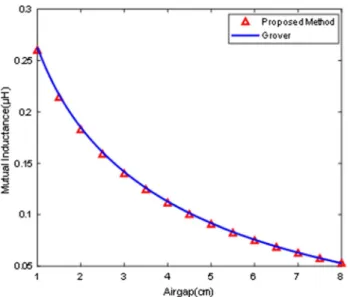
Since the Grover method can be used to calculate the mutual inductance between identical coils, the proposed method has been applied for two identical and single turn hexagonal coils with distances ranging from 1 to 8 cm between the primary and secondary coils of 20 cm side lengths. As shown in Fig. 6, the results of the proposed method well match with the Grover’s formula results. Grov-er’s extended formula gives more accurate results than its simple form which is given in (24). In addition, the approxi-mation to the mutual inductance between the identical hex-agonal coils with three number of turns, 10 cm air gap and
(24) M=0.012s � log �s d � − 0.151524 + d s � 1−𝜋 √ 3 9 � +d2 s2 � 2√3− 3 4 � −d4 s4 � 33√3− 46 216 + ⋯ ��
10 cm outer side lengths is obtained with an acceptable error rate which is a result of 112 iterations and given in Fig. 7.
4 Comparison of experimental, FEA
and analytical results for different coil
dimensions
As seen in the third section, the results of the methods in the literature are similar with the proposed method. In this section, the results obtained with the proposed method were compared with FEA and experimental results for dif-ferent coil dimensions. For this purpose, two hexagonal coils each with three turns in 10 and 20 cm outer side
Fig. 6 Comparison of mutual inductance calculation
Fig. 7 The variation of the mutual inductance value with the number of iterations
Fig. 8 3D FEA model and the manufactured hexagonal coils
Table 2 Comparison of FEA and experimental results with proposed method for self-inductance calculation
Self-inductance (µH) 2kout= 10 cm 2kout= 20 cm
Measured 4.64 10.67
FEA 4.51 10.54
Proposed Method 4.37 10.37
length dimensions are manufactured. The presentation of the coils manufactured in the laboratory and 3D model of the coils created with ANSYS Maxwell software are given in Fig. 8. Table 2 shows the comparison of the results obtained, with FEA and measured self-inductance values with the LCR meter in order to verify the self-inductance calculations of the manufactured coils. The frequency of the LCR meter was set to 20 kHz which is a common operating frequency for wireless power transfer systems. The LCR meter has 0.1% measurement accuracy as stated in the User Manuel. That means 0.01 µH error margin for a measurement of a coil with 10 µH value.
When the results obtained in Table 2 are examined, while the self-inductance values of the coil structures in the given dimensions are required to long calculation time by FEA, the recommended method can be calculated self-inductance values with small error rates as 2.8 and 5.8%, respectively. Considering the results obtained in this section and section three, it is thought that the proposed approach will have an important place in the literature because of the fact that the equations can be calculated with small error rates and the equations used have simple solutions.
In order to verify the mutual inductance calculations obtained by the proposed method, the distance between iden-tical coils with three turns was changed from 2 to 12 cm, and the results were compared with the FEA and the meas-ured results. Mutual inductance measurement procedure is as follows; First, the self-inductance values of the primary and secondary coils are measured with LCR meter and summed up. Then, one end of the primary coil and one end of the secondary coil are connected in series and a value is measured with the LCR meter. The summation of the self-inductances is subtracted from this and divided into two to get the mutual inductance value. In addition, the number of iterations required to obtain results at a predetermined error rate for each distance is given in Tables 3 and 4.
It can be seen obviously from Tables 3 and 4 that the proposed method results well match with the measurement results. In EV applications, the air gap between the coils is generally 10 cm and for this air gap the mutual inductance
value for two identical hexagonal coils with 20 cm outer side lengths is calculated with just 5.84% error rate when compared to actual measurement results. When iteration number is examined, it is necessary to have higher iteration numbers in order to obtain the same error rate in small size coils. The reason for this is that the ratio of neglected area value to total area has a more significant value in small size coils. As the distance between the coils increases, the increase in the percentage error of the calculated mutual inductance value can be explained by the increasing of the amount of leakage at the same time. Figure 9 shows the comparison of the obtained mutual inductance results for the proposed method, FEA and experimental measure-ments at different air gaps with 20 cm side lengths of two hexagonal coils. When taking into consideration the meas-urement conditions, the number of turns which is more than one and the occurrence of parasitic errors due to the connectors, the inductance calculations can be performed by using the new proposed method with small error rates.
Table 3 Mutual inductance calculation and comparison of results (2kout = 10 cm)
Air gap (cm) M (µH) Number of
iterations Error (%) Measured FEA Numerical
2 1.55 1.53 1.58 94 1.9 4 0.94 0.93 0.96 100 2.08 6 0.62 0.61 0.64 104 3.22 8 0.42 0.41 0.44 108 4.76 10 0.3 0.29 0.32 112 6.67 12 0.21 0.2 0.23 114 9.5
Table 4 Mutual inductance calculation and comparison of results (2kout = 20 cm)
Airgap (cm) M (µH) Number of
iterations Error (%) Measured FEA Numerical
2 4.48 4.6 4.63 91 3.50 4 3.12 3.2 3.25 94 3.63 6 2.38 2.41 2.48 97 4.13 8 1.87 1.89 1.97 100 5.31 10 1.51 1.52 1.6 102 5.84 12 1.24 1.25 1.32 104 6.29
5 Conclusion
In this study, a new method has been proposed by using sim-ple magnetic flux distribution formulas which can be used for self and mutual inductance calculations of hexagonal coil structures. In order to prove the accuracy of the proposed method, the obtained results are compared with experimen-tal measurements, FEA and different solution methods. The self-inductance value of the hexagonal coil with a side length of 20 cm calculated by the proposed method can be obtained with 2.8% error when compared to the experimental results. The distance between the coils is generally 10 cm in EV applications, and it is seen that the mutual inductance value can be obtained with 5.84% error for this distance when the proposed method result is compared with the experimental measurements. Considering that the inductance values are also large due to the size of the coils in these high-power applications, it is acceptable that these error rates will not cause a significant change in the number of turns. There are different approaches for inductance calculations in the litera-ture, and some of them have great accuracy, especially for the multi-turn and small-sized coils. However, they are using complex integrals and different coefficients which is a dis-advantage for these methods. Since with a simple approach, both the self and mutual inductance values can be obtained with acceptable error rates, the proposed method is a good candidate for the calculation of inductance values. For the future work, the proposed method can be used for inductance calculations of all polygons.
Acknowledgements This work has been conducted under the project contract 5160042 which is supported by Scientific and Technologi-cal Research Council of Turkey (TUBITAK). Authors wish to thank TUBITAK for this support.
Appendix
Magnetic flux density equation can be written by the Biot-Savart Law,
The total magnetic flux equation for calculating the tri-angle areas which are divided into recttri-angles, depending on the side length of the hexagon and the division parameters
n and i is can be obtained as follows,
(25) ⃗ B= 𝜇0I 4𝜋 1 r ⋅ � z+ k √ (z + k)2+ r2 − √ z− k (z − k)2+ r2 � ⋅ ̂𝜑
In order to simplify this complicated integration equation, we can divide it in four pieces and solve each part of it. As an example, only the solution of part A1 is given and the other
parts can be solved by the same approach.
Since there are two symmetrical triangles within the hex-agonal area, the sum of the total flux formed by the AB length is equal to the sum of the two triangular areas. Thus, the total flux equation of the triangles is,
Finally, the large rectangular area needs to be calculated. With the same approach, the total flux equation can be obtained if the integral boundaries are re-determined,
After simplification of the equations for calculating the self-inductance of a hexagonal coil, the total flux is,
(26) 𝜑AB= 𝜇0I 4𝜋 ∫ k√3(2n−i) n k√3i n ∫ k(n+i−1) n k(n+i−1) n z+ k √ (z + k)2+ r2 − √ z− k (z − k)2+ r2 ⋅dz ⋅ dr (27) 𝜑AB=𝜇0I 4𝜋 k√3(2n−i) n ∫ k√3i n 1 r ⋅ ⎡ ⎢ ⎢ ⎣ �� k(2n + i) n �2 + r2−��ki n �2 + r2 − �� k(2n + i − 1) n �2 + r2+ �� k(i − 1) n �2 + r2 ⎤ ⎥ ⎥ ⎦ ⋅ dr (28) 𝜑AB,Δ= 𝜇0I 4𝜋 ( A1− A2− A3+ A4) (29) A1= � � � � ��k(2n + i) n �2 + � k√3(2n − i) n �2 − k � (2n + i) n � ln ⎡ ⎢ ⎢ ⎢ ⎢ ⎣ �� k(2n+i) n �2 + � k√3(2n−i) n �2 + � k(2n+i) n � � k(2n+i) n � ⎤ ⎥ ⎥ ⎥ ⎥ ⎦ (30) 𝜑T,AB,Δ=2𝜇0I 4𝜋 ( A1− A2− A3+ A4) =𝜇0I 2𝜋 ( A1− A2− A3+ A4) (31) 𝜑AB,rectangular= 𝜇0I 4𝜋 ∫ 2k√3−rw rw 1 r ⋅ � ∫ k −k z+ k √ (z + k)2+ r2 ⋅ dz −∫ k −k z− k √ (z − k)2+ r2 ⋅ dz � ⋅ dr
By using this equation, the self-inductance for a hexago-nal coil for any size and wire radius is given by,
References
1. Zhang X, Ho SL, Fu WN (2013) A hybrid optimal design strategy of wireless magnetic-resonant charger for deep brain stimulation devices. IEEE Trans Magn 49(5):2145–2148
2. Zhang X, Yuan Z, Yang Q, Li Y, Zhu J, Li Y (2016) Coil design and efficiency analysis for dynamic wireless charging system for electric vehicles. IEEE Trans Magn 52(7):1–4
3. Budhia M, Covic G, Boys J (2010) A new IPT magnetic coupler for electric vehicle charging systems. In: IECON 2010—36th annual conference on IEEE industrial electronics society, Glen-dale, AZ, pp 2487–2492
4. Lin FY, Zaheer A, Budhia M, Covic GA (2014) Reducing leakage flux in IPT systems by modifying pad ferrite structures. In: IEEE energy conversion congress and exposition (ECCE), Pittsburgh, PA, pp 1770–1777
5. Wang CS, Covic GA, Stielau OH (2004) Power transfer capability and bifurcation phenomena of loosely coupled inductive power transfer systems. IEEE Trans Industr Electron 51(1):148–157 6. Wang Z, Wei X, Dai H (2016) Design and control of a 3 kW
wire-less power transfer system for electric vehicles. Energies 9:10 7. Moon S, Moon G (2016) Wireless power transfer system with an
asymmetric four-coil resonator for electric vehicle battery charg-ers. IEEE Trans Power Electron 31(10):6844–6854
8. Deng J, Li W, Nguyen TD, Li S, Mi CC (2015) Compact and efficient bipolar coupler for wireless power chargers: design and analysis. IEEE Trans Power Electron 30(11):6130–6140 9. Dehui W, Qisheng S, Xiaohong W, Fang C (2018) Calculation of
self- and mutual inductances of rounded rectangular coils with rectangular cross-sections and misalignments. IET Electr Power Appl 12(7):1014–1019
10. Dehui W, Qisheng S, Xiaohong W, Fan Y (2018) Analytical model of mutual coupling between rectangular spiral coils with lateral misalignment for wireless power applications. IET Power Electron 11(5):781–786
11. Grover FW (1922) Formulas and tables for the calculation of the inductance of coils of polygonal form. Sci Pap Bur Stand 18:737–762
12. Paul CR (2011) Inductance: loop and partial. Wiley, Hoboken 13. Aditya K (2017) Analytical design of archimedian spiral coils
used in inductive power transfer for electric vehicles application. Electr Eng 100(3):1819–1826
(32)
𝜑AB,total= 6(𝜑T,AB,Δ+ 𝜑AB,rectangular)
(33) Lhexagon= 6N 2(2𝜑 AB,Δ+ 𝜑AB,rectangular ) I
14. Jow U, Ghovanloo M (2013) Geometrical design of a scalable overlapping planar spiral coil array to generate a homogeneous magnetic field. IEEE Trans Magn 49(6):2933–2945
15. Xia CY, Zhang J, Jia N, Zhuang YH, Wu XJ (2013) Asymmetric magnetic unit of three-phase IPT system for achieving effective power transmission. Electron Lett 49(11):717–719
16. Tan P, Liu C, Ye L, Peng T (2017) Modeling and experimenta-tion of multi-coil switching coupler for wireless power transfer systems. In: IEEE energy conversion congress and exposition (ECCE), Cincinnati, OH, pp 2579–2583
17. Aydin E, Kosesoy Y, Yildiriz E, Timur Aydemir M (2018) Com-parison of hexagonal and square coils for use in wireless charging of electric vehicle battery. In: International symposium on elec-tronics and telecommunications (ISETC), Timisoara, Romania, pp 1–4
18. Peters C, Manoli Y (2008) Inductance calculation of planar multi-layer and multi-wire coils: an analytical approach. Sens Actuators A 145–146:394–404
19. Tavakkoli H et al (2016) Analytical study of mutual inductance of hexagonal and octagonal spiral planer coils. Sens Actuators A 247:53–64
20. Tan P, Yi F, Liu C, Guo Y (2018) Modeling of mutual induct-ance for hexagonal coils with horizontal misalignment in wireless power transfer. In: IEEE energy conversion congress and exposi-tion (ECCE), Portland, OR, USA, pp 1981–1986
21. Dalal A, Joy TPER, Kumar P (2015) Mutual inductance computa-tion method for coils of different geometries and misalignments. In: IEEE power and energy society general meeting, Denver, CO, pp 1–5
22. Greenhouse H (1974) Design of planar rectangular microelec-tronic inductors. IEEE Trans Parts Hybrids Packag 10(2):101–109 23. Mohan SS, del Mar Hershenson M, Boyd SP, Lee TH (1999)
Simple accurate expressions for planar spiral inductances. IEEE J Solid-State Circuits 34(10):1419–1424
24. Barmada S, Fontana N, Tucci M (2019) Design guidelines for magnetically coupled resonant coils with data transfer capability. In: International applied computational electromagnetics society symposium (ACES), Miami, FL, USA, pp 1–2
25. Song B, Cui S, Li Y, Zhu C (2020) A fast and general method to calculate mutual inductance for EV dynamic wireless charg-ing system. IEEE Trans Power Electron. https ://doi.org/10.1109/ tpel.2020.30151 00
26. Sallan J, Villa JL, Llombart A, Sanz JF (2009) Optimal design of ICPT systems applied to electric vehicle battery charge. IEEE Trans Industr Electron 56(6):2140–2149
27. Wheeler HA (1928) Simple inductance formulas for radio coils. Proc IRE 16(10):1398–1400
28. Rosa EB (1906) Calculation of the self-inductances of single-layer coils. Bull Bur Stand 2(2):161–187
Publisher’s Note Springer Nature remains neutral with regard to jurisdictional claims in published maps and institutional affiliations.