Optimal margins and price limits for future contracts

OPTIMAL MARGINS AND PRICE LIMITS FOR FUTURES CONTRACTS

A THESIS

SUBMITTED TO THE DEPARTMENT OF INDUSTRIAL ENGINEERING

AND THE INSTITUTE OF ENGINEERING AND SCIENCES OF BILKENT UNIVERSITY

IN PARTIAL FULFILLMENT OF THE REQUIREMENTS FOR THE DEGREE OF

MASTER OF SCIENCE

By

Altay Emre Poyraz August 2008

I certify that I have read this thesis and that in my opinion it is fully adequate, in scope and in quality, as a thesis for the degree of Master of Science.

Asst. Prof. M. Murat Fadıloğlu (Advisor)

I certify that I have read this thesis and that in my opinion it is fully adequate, in scope and in quality, as a thesis for the degree of Master of Science.

Assoc. Prof. Aslıhan Altay Salih

I certify that I have read this thesis and that in my opinion it is fully adequate, in scope and in quality, as a thesis for the degree of Master of Science.

Prof. Mustafa Ç. Pınar

Approved for the Institute of Engineering and Sciences:

Prof. Mehmet Baray

Director of Institute of Engineering and Sciences

ABSTRACT

OPTIMAL MARGINS AND PRICE LIMITS FOR FUTURES CONTRACTS

Altay Emre Poyraz M.S. in Industrial Engineering Supervisor: Asst. Prof. M. Murat Fadıloğlu

August 2008

Along with price limits, the margin mechanism ensures the integrity of futures markets. Exchanges face a trade-off between setting higher margin levels to protect the market from possible defaults and setting lower margin levels to make the market attractive to customers. In this thesis we develop a model to determine optimal margins and price limits for futures contracts, which minimizes the liquidity and margin costs to the traders while protecting the market from disruptions. Our model allows asymmetry between upper and lower price limits consequently between margins for long and short positions. We also provide a model, which is valid in the absence of price limits, to determine optimal margins and compare it with our previous model with price limits. The suggested model is applied to canola futures contract traded in Winnipeg Commodity Exchange (WCE) and comparable results to actual margin levels imposed by the exchange are obtained.

Keywords: Margin setting, price limits, futures markets, censored observations, GARCH estimation

ÖZET

VADELİ İŞLEM PİYASALARI İÇİN EN İYİ MARJLAR VE FİYAT SINIRLARI

Altay Emre Poyraz

Endüstri Mühendisliği, Yüksek Lisans Tez Yöneticisi: Yrd. Doç. M. Murat Fadıloğlu

Ağustos 2008

Vadeli işlem piyasaları olası kredi riskine karşı kendilerini fiyat limitleri ve marj mekanizması yoluyla korurlar. Borsalar kredi riskini en aza indirmek için yüksek marjlar belirleyebilirler, ancak bu durum yükselen maliyetler ile birlikte bu piyasalarda işlem yapan yatırımcı sayısını azaltan bir etki yaratabilir. Bu tezde yatırımcıların likidite ve marj maliyetlerini enküçülten ve aynı zamanda piyasayı taahhütlerin yerine getirilmemesi durumuna karşı koruyan bir model geliştirilmiştir. Modelimizde aşağı ve yukarı fiyat sınırları ve dolayısıyla da kontrattaki her iki tarafın marj miktarları arasında bakışımsızlık olması da hesaba katılmıştır. Ayrıca eniyi marjları belirlemek için fiyat sınırları olmadığı durumlarda geçerli olan bir model de geliştirilmiş ve bu model daha önceki fiyat sınırlı modelle kıyaslanmıştır. Önerilen model Winnipeg Mal Borsası’nda işlem gören kanola vadeli işlem kontratına uygulanmış ve yürürlükte olan gerçek marj seviyeleriyle kıyaslanabilir marjlar elde edilmiştir.

Anahtar sözcükler: Marj belirleme, fiyat sınırları, vadeli işlem piyasaları, sansürlenmiş gözlemler, Ardışık Bağlanımlı Koşullu Değişen Varyans (ABKDV) tahmini

ACKOWLEDGEMENT

I would like to express my gratitude to my advisor Asst. Prof. M. Murat Fadıloğlu for all the trust and encouragement and to Assoc. Prof. Aslıhan Altay Salih for her instructive comments and support.

I am indebted to Prof. Mustafa Ç. Pınar for accepting to read and review this thesis and for his invaluable suggestions.

Finally, I would like to express my special thanks and gratitude to TÜBİTAK for the scholarship provided throughout the thesis study.

CONTENTS

1 Introduction ...1

2 Margin and Price Limit Mechanisms...6

3 Literature Review...9

4 Theoretical Models for Margins and Price Limits ...13

4.1 Brennan's Model ...13

4.2 Shanker and Balakrishnan's Model ...16

4.3 Model...18

4.3.1 Model for Long Position...19

4.3.2 Model for Short Position...19

4.4 A Comparable Model Without Price Limits ...21

4.4.1 Model for Long Position in the Absence of Price Limits ...21

4.4.2 Model for Short Position in the Absence of Price Limits...21

5 Model Specifications and Algorithm ...23

5.1 Objective Function...23

5.2 Self-Enforcing Property ...24

5.3 Controlling Probability of Hitting the Limit ...25

5.4 Estimation of the Censored Data ...25

5.5 Our Algorithm in Determining Margins and Price Limits ...28

6 Empirical Results ...29

6.1 Properties of Data Used ...29

6.2 Estimation of the Distribution Parameters ...31

6.3 Determining Optimal Margins and Price Limits with Various Tolerable Default Probabilities...33

6.4 Weekly Optimal Margins and Price Limits with Chosen Tolerable Default Probabilities...36

6.5 Comparison of the Model with Price Limits and the Model in the Absence of Price Limits ...41

7 Conclusion...43

Bibliography...46

LIST OF FIGURES

6-3-1: The relationship between tolerable probability and margin; tolerable probability and price limit for the last day of period 1 ...34

6-3-2: The relationship between tolerable probability and margin of long position; tolerable probability and lower price limit for the last day of period 2...35

6-3-3: The relationship between tolerable probability and margin of short position; tolerable probability and upper price limit for the last day of period 2...35

6-3-4: The relationship between tolerable probability and margin; tolerable probability and price limit for the last day of period 3 ...36

6-4-1: Optimal weekly margin differences between long and short positions after the 29th week of period 2 with tolerable probability of 0.5%...38

6-4-2: Optimal weekly margin differences between long and short positions after the 29th week of period 2 with tolerable probability of 2.5%...39

6-4-2: Probability of exceeding price limit p used versus expected margin exceeding C for the last day of period 3...42

LIST OF TABLES

6-1: Characteristics of canola futures contract traded in WCE for three periods ...30

6-2: Averages and standard deviations of GARCH parameters for three periods ...32

6-4-1: Averages of actual and optimum margins and price limits of canola futures contract with tolerable probabilities of 0.5% and 2.5% ...37

6-4-2: Averages of excess margins that would be paid by the traders for canola futures contract if our optimal margins were applied by the exchange for three periods ...40

C h a p t e r 1

INTRODUCTION

In future contracts, two parties, namely short and long positions, agree to trade an asset in the future for a certain price and delivery conditions. However, exchanges specifically the clearinghouse bears the credit risk due to a default by one of the parties. In an attempt to control for the default risk margin mechanism is imposed.

Although there are exceptions like crude oil and gold, exchanges usually set daily price limits for future contracts. Price limits are mechanisms that aim to restrict extreme movements in the market. In addition, these limits may serve as partial substitutes for margins by reducing the margin requirements (Brennan, 1986; Chou et al., 2000). Once a futures price hits the daily price limit, trading ceases and there can be no trading at any higher price until the next trading day.

Determining price limits and setting margin levels for futures contracts are important problems for exchanges. Setting high margin levels can provide safety by minimizing the risk of default, which occurs when the futures price change exceeds margin deposited by the trader and margin call is not fulfilled by him, but it results in a decrease in the volume of the traded contracts. On the other hand, setting lower margin levels increases the

CHAPTER 1. INTRODUCTION 2 attraction to the exchange by traders. In addition to margins, setting price limits is also a problem, because when the price of a contract hits the price limit then trading ceases and price limits become effective barriers for traders.

In this thesis we develop a model to find optimal margins and price limits for futures contracts, while minimizing the cost to the traders and at the same time providing protection to the market against default risk. Our model is specifically based on the works of Brennan (1986) and Shanker and Balakrishnan (2005).

According to Brennan (1986) an efficient contract minimizes the total cost for market participants. Therefore, he develops a theoretical model that minimizes these costs, which includes the opportunity cost of margin, cost of the limit that arises when a limit move occurs and cost of reneging. Cost of the limit and cost of reneging are not measurable costs, so instead of solving his model, Brennan makes an analysis of the model for various margins and price limits. Reneging can occur when the trader believes that the change in the futures price exceeds his margin. Setting price limits can reduce the risk of reneging, because price limits constrain the information available to the trader. Since the trader cannot see the actual price, he is not sure about how much the change in the future price will exceed his margin. As a result, the trader’s decision is based on the conditional expected loss when price limit is hit. Brennan also argues the ‘self-enforcing’ property, under which the parties of the contract obey its terms and he denotes that a contract can be made ‘self-enforcing’ by setting margin and price limits such that when price limit is hit the expected loss of the trader is below or equal to the trader’s margin level.

CHAPTER 1. INTRODUCTION 3 Shanker and Balakrishnan (2005) extend the model of Brennan; however they exclude the non-measurable costs like cost of the limit and cost of reneging; instead they minimize only the opportunity cost of margin and capital contribution of the trader, which makes their model more applicable. Like Brennan they assume that “the optimal contract is self-enforcing” and formalize their model accordingly. On the other hand, different from Brennan they control the liquidity cost (i.e. cost of hitting price limit) by restricting the probability of hitting price limit by a desired value. Since the prices of the market can move only within certain limits the whole series of the prices has a censored distribution. In order to overcome the effects of censoring they use a generalized autoregressive conditional heteroskedastic (GARCH) model as well as maximum likelihood methods. They apply their model to the canola futures contract traded in Winnipeg Commodity Exchange (WCE) for two periods; the first of which extends from January 3, 1995 to December 31, 1997 and the second extends from January 4, 1999 to December 31, 2001 and they estimate daily margins, capital contributions and price limits for these two periods.

We extend the models of Brennan (1986) and Shanker and Balakrishnan (2005) by quantifying the liquidity cost for traders in long and short positions and estimating asymmetric margins and price limits if there is a significant difference between the up and down price movements; i.e. if the volatilities between up and down price movements are significantly different from each other. If price limit is hit, then the winning party of the contract cannot realize his profit above the price limit on that day. Therefore, we try to minimize this cost arising from hitting the price limit. Moreover, futures prices can behave differently in up and down movements resulting in different risk levels for short and long positions. Although Longin (1999)

CHAPTER 1. INTRODUCTION 4 states that asymmetry is not preferred by some exchanges like Chicago Board of Trade and London Clearing House, we think that large differences between up and down price movements may result in an inequality among market participants, when they put identical margin amounts. Thus, we treat long and short positions differently in order to obtain asymmetric margins and price limits if the difference between up and down price movements is significant.

Our model aims to minimize the opportunity cost of the market participants due to margin requirement and market disruptions caused by the introduction of price limits. Just as Brennan (1986) and Shanker and Balakrishnan (2005), we assume that “an efficient contract should exhibit the self-enforcing property”; also like Shanker and Balakrishnan we constrain the probability of hitting the price limit, but instead of assigning an exact value we solve our model with different probability levels. We use the GARCH based algorithm developed by Morgan and Trevor (1999) to overcome the effects of censoring. We apply our model to the Canola futures contract traded in Winnipeg Commodity Exchange for the two periods (January 3, 1995 to December 31, 1997 and January 4, 1999 to December 31, 2001) used also by Shanker and Balakrishnan (2005) as well as a more recent third period that extends from January 2, 2004 to December 29, 2006 to estimate weekly margins and price limits for the last year of each period. We obtain results comparable to actual levels. Furthermore, instead of daily setting, we determine weekly margin levels and price limits which decreases calculation efforts and is easier to apply.

Although price limit mechanism is crucial for self-enforcement and it acts as a partial substitute for margins, exchanges do not set price limits for some

CHAPTER 1. INTRODUCTION 5 future contracts like crude oil and gold. Therefore, we develop another model which is valid in the absence of price limits and compare it with our initial model.

The thesis is organized in seven chapters. Next chapter explains futures contract mechanism and gives the necessary background in order to follow this thesis. Chapter 3 discusses the literature; Chapter 4 and 5 present our model and solution methodology respectively. Chapter 6 includes presentation of our results for the three periods. Finally, Chapter 7 concludes and addresses future research directions.

C h a p t e r 2

MARGIN AND PRICE LIMIT

MECHANISMS

In this section some important concepts are introduced1 to give the necessary background in order to follow this thesis2.

A futures contract is an agreement to buy or sell an underlying asset with a certain price at a certain time in the future. Let us consider an airline company that is trying to protect itself from adverse price fluctuations in jet fuel oil and wants to fix the price of oil it will need for the next three months. Similarly, an oil company also has concerns about the fluctuating oil prices and wants to sell its oil in the market from a fixed price three months from now. These two companies can engage in a futures contract agreement through a derivatives exchange. The contract specifies the quality, price, quantity of oil that will be delivered three months from now under specified delivery conditions. Here, the airline company, the buyer of the underlying asset (oil), holds the long position and the oil company, the seller of oil, holds the short position. The

1 _{This section can be omitted by the reader who has knowledge about the futures margin and price limit}

mechanisms.

2 _{See Hull (1991) for more details and examples.}

CHAPTER 2. MARGIN AND PRICE LIMIT MECHANISMS 7 price these companies agree to buy and sell oil via the futures contract from the exchange is called the futures price.

If the future price increases then the airline company benefits, as the price it agreed to buy the oil remains below the market price at the delivery date. Similarly, when the futures price falls, the oil company benefits, since the price it agreed to sell its product is higher than the market price.

In the futures contract agreement one of the parties may default on the contract. In order to shield the market participants from the default risk, the clearinghouse guarantees the counter party risk by taking the opposite side of each contract. However, carrying this default risk requires a protection mechanism and derivative exchanges use price limits and margin mechanism to that purpose. Margin, which is typically 5%-15% of the contract’s value, is simply a deposit that should be paid by the traders in order to take a position in a futures contract agreement, it can be seen as a collateral for expected losses. At the end of each trading day the gain or loss of the trader is reflected into his margin account. This process is called marking to market. If the amount in the margin account of the trader falls below the initial margin level then he receives a margin call to restore the amount in the account to its initial level. If the trader does not obey the margin call his position is closed by the exchange.

To illustrate how margin mechanism works, consider an oil futures contract traded in an exchange. Suppose that the price of the contract is $200 per barrel of oil and the contract size is 100 barrels. Moreover, suppose that margin is $1,000. Both the traders in long and short position should deposit this amount as margin in order to enter this oil futures contract agreement. For example, if the futures price drops to $198 per barrel at the end of the trading day, the

CHAPTER 2. MARGIN AND PRICE LIMIT MECHANISMS 8 balance in the margin account of the long position drops to $800 and similarly the balance in the margin account of the trader in short position rises to $1,200. On the contrary, if the futures price rises to $203 per barrel at the end of the trading day, the balance in the margin account of the long position increases to $1,300 and similarly the balance in the margin account of the trader in short position falls to $700.

After these adjustments, depending on the amount in the margin accounts, some traders receive a margin call. In the above example, when the price of the futures contract falls to $198 per barrel, then the trader in long position receives a margin call to restore his margin amount to $1,000, which is the initial margin level. Similarly, the trader in short position receives a margin call when the price of the futures contract rises to $203 per barrel.

Derivative exchanges also impose a maintenance margin, which is below the initial margin level, and allow the balance in the margin account to diminish to that level. When the balance in the margin account hits the maintenance margin level the trader receives a margin call, and he needs to recover his margin account up to the initial margin level.

Price limits are maximum allowable price changes of futures contracts. When the limit is hit trading ceases and no trading will be allowed until the next day. Following the oil example, suppose that price limits are set as $5 for up and down movements, which means that the price of oil futures cannot fall under $195 and rise above $205. Then, maximum gain or loss of a trader who holds one oil futures contract will be $500.

C h a p t e r 3

LITERATURE REVIEW

Derivative exchanges face a dilemma about setting the level of margin. In order to attract more investors and increase the liquidity in the market, the margin level should be set as low as possible, however the level of margin should be enough to cover most of the losses that could be incurred within a day. Telser (1981) examines margins from an economic theory perspective and he discusses the reasons behind the margin mechanism and effects resulting from changes in the margin levels. He argues that margin is a mechanism that reflects the self-interest of agents who wish to protect themselves against losses. Moreover, he agrees that an increase in the margin level can reduce the liquidity of the market, due to the higher cost of trading. Hartzmark (1986) studies the effects of margin level on trader’s investment decision and shows theoretically that margin level plays an important role in determining the demand to the contract, contract price and volatility. He argues that exchanges should keep margin requirements as low as possible to keep market liquid. The relationship between margin level and the demand to the market is also studied by Ma et al. (1993). They investigate the effects of margin change in the silver futures markets and conclude that significant changes in market trading activity are associated with changes in margin levels.

CHAPTER 3. LITERATURE REVIEW 10 On the other hand, setting low margin levels increases the default risk. Figlewski (1984) works on margins requirements on stocks and equity based derivatives and focuses on setting margins. He develops a technique, which uses the mean return and volatility of security prices, the margin requirement and the period allowed after the margin call to calculate the probability of margin violation within a given number of days. Gay et al. (1986) contributes to Figlewski (1984) and argue that margins should be set by the exchange so that in a given time interval the probability of exceeding margin should be the same for all future contracts.

Exchanges use different methods in setting margins. Chicago Mercantile Exchange (CME) uses a complicated system called SPAN, which works on possible scenarios to determine margins. Kupiec (1994) analyzes the margins requirements of S&P futures under the SPAN margining system of Chicago Mercantile Exchange and states that SPAN margining system is more efficient than the strategy-based system that was applied before by the exchange. Bates and Craine (1999) examine the Futures Market Clearinghouse's default exposure during the 1987 Crash and also conclude that SPAN margining system introduced after the Crash in 1988 is more successful in setting appropriate margins compared to the previous system.

Despite the methods used by the exchanges, various methods were developed to determine margins and price limits. Ackert and Hunter (1994) test a simple optimization model of daily price limits assuming that exchanges are operating under the criteria of minimizing the long run average cost. Their optimal results are equal to the average price limits imposed by the exchange. Fenn and Kupiec (1993) compare different margin policies of clearinghouses, which are designed to minimize future contract

CHAPTER 3. LITERATURE REVIEW 11 costs that include margin cost, settlement cost and the cost of allowing a deficit to arise in a clearing member’s margin account and they argue that clearinghouses are not keeping in mind the cost-minimization in setting margins for stock-index futures. Dutt and Wein (2003) perform a simulation to test alternative margin setting methodologies. They state that exchanges should consider the preferred probability of customer account exhaustion in setting margins. Lam et al. (2004) compare different margin-setting methodologies, all of which strike a balance between setting prudential margin levels and minimizing the cost of margin. They test three margin-setting methodologies, namely simple moving averages; exponentially weighted moving averages and GARCH approach and GARCH outperforms in their study. Longin (1999), Dewachter and Gielens (1999), Broussard (2001), Cotter (2001) and Cotter and Dowd (2006) use methods in setting optimal margins by using the extreme value theory. Since margins should cover the risks arising from extreme price changes, they focus on the tails of the futures price distribution. Edwards and Neftci (1988) state that in setting margins exchanges should consider the correlations between different commodities and argue that if extreme future price movements in different commodities are correlated then this relationship should be taken into account in setting margins. They find a statistically significant relationship between extreme price changes of different commodities.

Exchanges usually set price limits for futures contracts. The price limit mechanism ensures that the change in future prices remains within certain limits and behave as partial substitutes for margins as Brennan (1986) argues. Moreover, Chou et al. (2000) examine the problem of “can price limits reduce default risk and margin requirements for a self-enforcing futures contract?” and find out that when traders do not receive additional

CHAPTER 3. LITERATURE REVIEW 12 information, price limit can reduce the margin level.

C h a p t e r 4

THEORETICAL MODELS FOR

MARGINS AND PRICE LIMITS

The problem of setting optimal margins and price limits has been studied by various models as discussed earlier. Our approach borrows from the works of Brennan (1986) and Shanker and Balakrishnan (2005). Brennan’s theoretical model aims to find the optimal margin that protects the exchange from possible defaults by minimizing the opportunity cost of margin kept in the account and penalizing the lost liquidity due to the price limit and reneging by the investor when loss exceeds the margin kept in the account. He argues that a futures contract should be self-enforcing and he sets up his optimization model to ensure self-enforcement. The model proposed by Shanker and Balakrishnan (2005) modifies and operationalizes Brennan’s theoretical work. It is not possible to estimate the costs related to the lost liquidity and reneging in Brennan’s model, which prohibits a practical application of the model. Shanker and Balakrishnan (2005) propose a modified model that ignores reneging and controls the liquidity costs by constraining the probability of hitting a price limit to a tolerable level by the exchange.

4.1. Brennan’s Model

Brennan’s model is as follows:

CHAPTER 4. THEORETICAL MODELS FOR MARGINS AND PRICE LIMITS 14 Minimize KM + γ ) ~ Pr( ) ~ Pr( L X L X ≤ ≥ + 2 Pr(~ ,~ *( , )) (1) M L Y Y L X ≥ ≥ α such that,

[

]

Here, P_t−1 is the observed futures price at time t-1; P~_t is the equilibrium futures price that would have been observed in the absence of price limits at time t, X~ is the random futures price change from the previous day without price limits (P~_t −P_t−1). M represents margin and L is the price limit.

The first term in the objective function represents the opportunity cost of capital and K is the cost of tying a monetary unit to the margin. Second term is an attempt to penalize the lost liquidity. Here γ is the unit cost for the market disruption ratio calculated by dividing the probability of hitting the limit to the probability of no limit move. The third term in the objective function refers to the cost of reneging. Here, Y~ is the market signal, which is correlated with

X~, that the trader observes. is the critical value beyond which the trader reneges. The probability that the trader reneges ( *_{( , )} Y L M )) , ( ~ , ~

Pr(_{X ≥LY ≥Y}* _{L M ) is multiplied with two because of the symmetry for}

up and down price movements and this probability is also multiplied with α, which is the fixed cost incurred when the trader reneges.

The costs related to reneging and liquidity (α and γ) cannot be directly estimated. As Brennan argues there is no formal theory that will help us to determine these costs. Brennan utilizes his model for operational purposes, but examines its stipulations under different settings, e.g., with external

CHAPTER 4. THEORETICAL MODELS FOR MARGINS AND PRICE LIMITS

15 information, with no external information, with uniformly distributed price changes, and with normally distributed price changes.

The only constraint in the optimization model insures that the contract is self-enforcing. The self-enforcing property proposed by Brennan makes certain that a risk-neutral trader does not have any incentive to break the contract. Thus, under such conditions the futures market should have to worry about traders not honoring the term of their contracts. The mechanism through which the property is ensured is as follows: when price hits the limit, the trader cannot be sure about how much the actual price movement exceeds his margin. Since the trader has limited information about the actual price change because of the censoring effect of the limits, a risk-neutral trader can only decide on whether to honor the contract according to the expected price movement. The main premise of self-enforcing contracts is only valid given that there is no additional information on the actual price, i.e., no market signal. Brennan concludes that, in order for a contract to be self enforcing, there is one necessary and sufficient condition for each party, which is:

[

]

E ~_t − _t−1| ~_t − _t−1 ≤ ≤ (3)

for long position, and

[

]

E ~_t − _t−1| ~_t − _t−1 ≥ ≤ (4)

for short position. Pt-1 represents the price of the futures contract at time t-1

and Pt is the uncensored futures price at time t in the absence of the price

limits. Assuming symmetry in futures price distribution, inequalities (3) and (4) can be written as:

CHAPTER 4. THEORETICAL MODELS FOR MARGINS AND PRICE LIMITS

16

[

]

E ~_t − _t−1| ~_t − _t−1 > ≤ (5)

Brennan argues that cases where (5) holds as a strict inequality cannot be optimal, so he uses (5) as equality in his model (See equation (2)).

In his work, Brennan states that price limits can be partial substitutes for margins and they reduce the margin requirements.

4.2. Shanker and Balakrishnan’s Model

Shanker and Balakrishnan (2005) extend the model of Brennan and make it operational. Their model can be illustrated as follows:

Minimize (M_S +C_S(M_S))k+(M_L +C_L(M_L))k (6) subject to,

[

]

[

]

In this model, and represent upper and lower price limits and similarly and represent margins deposited by a clearing firm regarding to short and long futures positions respectively and k is the interest rate. Moreover, and are the capital contribution by the

U L L_L S M M_L ) ( _S S M C C_L(M_L)

CHAPTER 4. THEORETICAL MODELS FOR MARGINS AND PRICE LIMITS

17 clearing firm for short and long positions. This capital contribution is used to cover the losses arising from trader defaults when the losses exceed initial margin levels. Therefore capital contributions should be equal to the expected price change above the margin level.

In the model specified above, Shanker and Balakrishnan try to minimize the margin and capital deposited by clearing firm for both and short positions simultaneously with respect to , , and . Since both the margin and the capital contribution is paid by the clearing firm and they are both used as collateral against the risks due to price fluctuations, there is no need to distinguish them from an optimization perspective. The model would optimize the total amount

L

M M_S L_U L_L

( )

L L L

M +C M (and M_S +C M_S( _S)) and then the amount can be distributed between the margin and the capital contribution. This is the approach used in our own model as well as the one in Brennan (1986).

The main rationale behind the constraints (7), (8), (9) and (10) is based on the ideas of Brennan regarding to self-enforcing property. As stated in the discussion on Brennan’s model, a self-enforcing contract requires that margin should be greater than the limit and when the limit is hit the expected difference between the uncensored futures price at time t and futures price at time t-1 should be equal to the margin amount.

In order to make their model operational, Shanker and Balakrishnan do not use costs that are not easy to quantify such as cost of reneging and cost of the limit like Brennan does. They do not punish reneging; on the other hand instead of using a liquidity cost they control the liquidity by restricting the

CHAPTER 4. THEORETICAL MODELS FOR MARGINS AND PRICE LIMITS

18 total probability of exceeding the upper and lower price limits by a probability

p.

Indeed the model of Shanker and Balakrishnan allows asymmetry, however they solve their model as symmetric and obtain equal margins for long and short positions as well as equal price limits for up and down movements. The main rationale behind this is the assumption used for the distribution of the futures prices. In addition, they estimate only one conditional variance which is valid for both up and down price movements.

Shanker and Balakrishnan apply their model to the canola futures contract traded in Winnipeg Commodity Exchange (WCE) for two periods, which extend from January 3, 1995 to December 31, 1997 and January 4, 1999 to December 31. They solve their model by taking p as 1% and k as daily interest rate on 3-month Canadian Treasury bills to determine optimal levels of daily margin, capital and price limits. Average values of optimal margins are higher in both periods, but optimal price limits are higher in period 1 but lower in period 2.

4.3. Model

We propose two separate models for long and short positions instead of solving a unified model for both. Let , represent margins of long and short positions; and represent upper and lower price limits; and are probabilities of hitting the lower and upper price limits respectively. Our models include the trader’s cost in their objective functions, while incorporating futures market’s concerns in the constraints. Our model is as follows:

L

M M_S

U

CHAPTER 4. THEORETICAL MODELS FOR MARGINS AND PRICE LIMITS

19

4.3.1. Model for Long Position

Minimize

(

)

[

]

4.3.2. Model for Short Position

Minimize

(

)

[

]

Our model possesses two important properties. The first important property of our model is that it allows asymmetry between long and short positions. If there is a significant difference between up and down price movements then we solve the related models stated above for long and short positions. In case that a significant difference is not present between up and down price movements then one of the models (either model for long position or model

CHAPTER 4. THEORETICAL MODELS FOR MARGINS AND PRICE LIMITS

20 for short position; does not make any difference) is solved and symmetric margins and price limits are obtained. Although Longin (1999) argues in his work that asymmetry between margins and price limits is not preferred by the exchanges because they think it results in inequalities among market participants, we think that in the case the price dynamics are different to treat long and short positions equally would be a source of inequality itself. When there is a significant difference between up and down price movements, it means that the volatility measures are different. Therefore, it would be unfair if the same amounts of margins were paid by long and short contract owners.

Second, we quantify “cost of the limit” in terms of the traders and include it in the objective function so that the objective function is the total cost incurred by the investor due to margin requirements and market disruptions caused by the presence of the price limits. When the futures contract hits the upper price limit, trading ceases and therefore the trader in long position cannot realize his true profit that day. In other words, the trader in long position would gain more than the amount of the limit if there were no limit since the unrestricted actual price would occur beyond the price limit. Similarly, the trader in short position cannot realize his true gain on a day when the price hits the lower price limit. The cost of disruption is the opportunity cost of not obtaining the potential gain on the days when price limits are exceeded. These costs constitute the second terms in the objective functions of both models for long and short positions.

As in Brennan (1986) and Shanker and Balakrishnan (2005), the opportunity cost of margin for both long and short positions is part of the objective function. In addition, putting a constraint providing M>L is redundant, because (13) and (17) already satisfy this requirement. Finally, like Shanker

CHAPTER 4. THEORETICAL MODELS FOR MARGINS AND PRICE LIMITS

21 and Balakrishnan we do not use cost of reneging for a couple of reasons. First, under the self enforcing constraint, the investors should not have any motive for reneging from the contract. Secondly, this cost would be hard to quantify as confessed by Brennan. Finally, since our objective function consists of the total cost experienced by the investor, it would not be meaningful to include this cost which is experienced by the futures market. In the model, we also constrain the probability of hitting the limit by a percentage in order to control the liquidity and we think that determination of this percentage should be made by the exchange.

4.4. A Comparable Model without Price Limits

Exchanges usually set price limits on futures contracts; however some futures contracts like crude oil and gold have no price limits. We develop a comparable model, which can be applied in the absence of price limits. This model can be summarized as follows:

4.4.1. Model for Long Position in the Absence of Price Limits

Minimize kM_L (20) subject to,

[

]

4.4.2. Model for Short Position in the Absence of Price Limits

Minimize kM_S (23)

CHAPTER 4. THEORETICAL MODELS FOR MARGINS AND PRICE LIMITS 22

[

]

In this model, the objective is minimizing the opportunity cost of margin and the expected loss of exceeding margin is limited with a tolerable value (CS or CL), which should be determined by the exchange like the tolerable

probabilities of the model with price limits.

In the absence of price limits self-enforcement cannot be achieved since price changes of futures contract can exceed the margin level imposed by the exchange. Therefore, CS and CL can also be considered as a pool of the

clearinghouse to backup the losses arising from defaults, when price changes exceed margin amounts.

C h a p t e r 5

MODEL SPECIFICATIONS AND

ALGORITHM

Let x~ be the uncensored return at time t and_t f(~x_t) be the probability density

function of the unrestricted futures return. We specify the objective function and the constraints in terms of x~ and_t f(~x_t)3.

5.1. Objective Function

Cost of the limit in objective functions can be rewritten for long and short positions respectively as:

(

∫

∫

∫

3 _{For detailed explanation of rewriting the equations in terms of}

t

x~ and f(~x_t)see Shanker and Balakrishnan (2005).

CHAPTER 5. MODEL SPECIFICATIONS AND ALGORITHM 24 (

∫

∫

∫

Parts after the parentheses represent probability functions in the objective function and after making necessary simplifications equations become

∫

∫

for long and short positions respectively.

5.2. Self-Enforcing Property

Equations (13) and (17) regarding to the self enforcing property can be rewritten as:

∫

∫

CHAPTER 5. MODEL SPECIFICATIONS AND ALGORITHM 25

∫

∫

5.3. Controlling Probability of Hitting the Limit

Probabilities of hitting upper and lower price limits are restricted by probabilities and , which should be determined by the derivatives exchange as their tolerable limit. Equations (14) and (18) regarding to these probabilities in terms of L p p_U t x~ and f(~x_t) are:

∫

∫

5.4. Estimation of the Censored Data

We employ Generalized Autoregressive Conditional Heteroskedasticity (GARCH) model4 of Engle (1982) and Bollerslev (1986) while estimating volatility of future returns series. GARCH5 model is used very commonly in the literature as Baillie and Myers (1991) show that these models are effective

4 _{For detailed explanation see Greene (2008).}

CHAPTER 5. MODEL SPECIFICATIONS AND ALGORITHM 26 in describing the distribution of future prices. GARCH model considers the variance of the current error term to be a function of the variances of the previous time period's error terms. This process can be illustrated as follows:

t t R =μ +ε (34) 2 2 2 2 2 1 1 0 2 _... n t n t t t =α +α ε − +α ε − + +α ε − σ (35)

Here Rt denotes the daily returns; μ is the mean of returns, is the surprise

component of the returns, is the conditional variance at time t and t ε 2 t σ n α α

α₀, ₁,..., are the coefficients of the variance equation, which are variables that need to be estimated. In GARCH process, coefficients of the conditional variance equation (34) are estimated by maximizing the following log-likelihood function:

∑

where T is the number of observations.

In solving our model the conditional distribution of futures returns are assumed to be normal. While using GARCH framework normal distribution assumption about the conditional density of commodity futures returns is very convenient and allows for time dependent conditional variances and leptokurtosis in the unconditional distribution of returns as argued by Baillie and Myers (1991). This assumption is inline with the documented finding of the unconditional distribution of the commodity returns being fat-tailed and

CHAPTER 5. MODEL SPECIFICATIONS AND ALGORITHM 27 leptokurtic in the literature6. Therefore, we decided to use the conditional normality assumption for futures returns, which is also operationally very convenient.

In determining the margins and price limits for future contracts one of the main problems is the estimation of the censored data. When prices hit the limit, it is not possible to observe the equilibrium prices that would have been prevailed. We employ the GARCH based model of Morgan and Trevor (1999), who use a rational expectations (RE) algorithm, which estimates the conditional expectations of the squares of the underlying equilibrium error terms, and simultaneously updates the GARCH process, to reflect the information on the unobserved equilibrium price revealed by the observed censored price.

Futures return volatility might react differently to positive and negative surprises and exhibit asymmetric property. In order to account for this possible asymmetry we use the following GARCH representation proposed by Glosten, Jagannathan and Runkle (1993):

2 3 2 2 2 1 0 2 1 t t t t t α α ε α σ α γ ε σ ₊ = + + + (37)

where and represent conditional variance and error term at time t respectively. 2 t σ 2 t ε 0

α , α₁, α₂ and α₃ are GJR-GARCH parameters.γ_t takes the value 1 if εt <0 and 0 otherwise.

CHAPTER 5. MODEL SPECIFICATIONS AND ALGORITHM 28 In case of an asymmetry in futures return data, we evaluate different variances for up and down movements. For a possible up (down) price movement we estimate the volatility by assigning 0 (1) to γ_t. Therefore we get two separate volatilities for up and down movements in the price while calculating the margins and price limits.

5.5. Our Algorithm in Determining Margins and Price Limits

Our algorithm to determine optimal margins and price limits can be summarized as follows:

• First, check the time series whether it has asymmetry or not by applying GJR-GARCH and testing the statistical significance of γ_t.

• Second, use the RE algorithm by Morgan and Trevor (1999) to estimate weekly unrestricted means and variances when asymmetry is detected in the data, estimations are conducted by using GJR-GARCH.

• Finally, solve the related models outlined in equations 12 to 19 to calculate optimal margins for both long and short positions and price limits for up or down price movements.

In order to determine the optimal margins and price limits for the first week of the last year of each period, the first two years data is used. Then for each week, the data set is expanded by one week and again the algorithm is used to calculate optimal margins and price limits.

C h a p t e r 6

EMPIRICAL RESULTS

6.1. Properties of Data Used

We use the data of the Canola futures contract which is traded in Winnipeg Commodity Exchange (WCE). The data is obtained from the website of WCE7. Canola oil futures data is used in this study as it is available through the exchange and WCE imposes price limits and changes margins for this contract from time to time. Therefore we have the opportunity of testing our model in periods with different price limits and margins. The first two periods of this data set is also used by Shanker and Balakrishnan (2005) which gives us a comparison base for our model.

We apply our model to three periods, first period extends from January 3,1995 to December 31, 1997 (period 1); the second one covers the January 4, 1999 to December 31, 2001 (period 2) and the last period is from January 2, 2004 to December 29, 2006 (period 3). Futures return series are obtained from the prices of the futures contract, using the nearby futures contract series excluding the observations in the delivery month and the days with 0 trading volume. In period 1, the actual price limits and margins imposed by the

7 _{www.wce.ca. The website is moved to www.theice.com.}

CHAPTER 6. EMPIRICAL RESULTS 30 exchange are both $10/tonne. In period 2, until 9 October, 2000 price limit is $10/tonne and $30/tonne afterwards. In addition, margin is updated monthly by Winnipeg Commodity Exchange (WCE) and it is a percentage of the daily settlement price. These percentages are computed by nearest futures settlement price × 2 × maximum of standard deviations of daily returns of past 20, 90 and 260 days’ of nearby contract. Price limit is $30/tonne and margins are updated

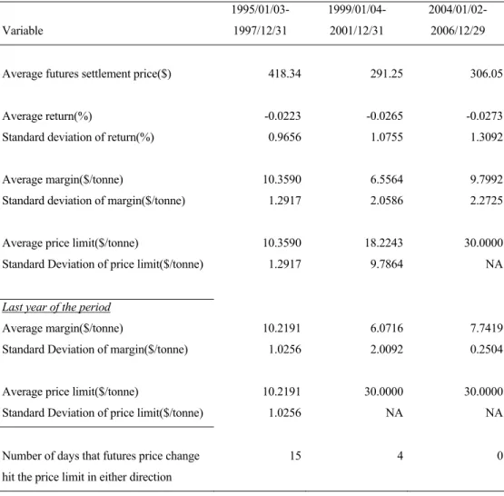
TABLE 6.1: Characteristics of canola futures contract traded in WCE for three periods Variable 1995/01/03-1997/12/31 1999/01/04-2001/12/31 2004/01/02-2006/12/29

Average futures settlement price($) 418.34 291.25 306.05

Average return(%) -0.0223 -0.0265 -0.0273

Standard deviation of return(%) 0.9656 1.0755 1.3092

Average margin($/tonne) 10.3590 6.5564 9.7992

Standard deviation of margin($/tonne) 1.2917 2.0586 2.2725

Average price limit($/tonne) 10.3590 18.2243 30.0000

Standard Deviation of price limit($/tonne) 1.2917 9.7864 NA

Last year of the period

Average margin($/tonne) 10.2191 6.0716 7.7419

Standard Deviation of margin($/tonne) 1.0256 2.0092 0.2504

Average price limit($/tonne) 10.2191 30.0000 30.0000

Standard Deviation of price limit($/tonne) 1.0256 NA NA

Number of days that futures price change 15 4 0

CHAPTER 6. EMPIRICAL RESULTS 31 monthly by the exchange in period 3. Before October 9, 2000 exchange expanded the price limits and margins by 50% depending on the limit moves of the nearest future contracts on the previous day. Table 6.1 summarizes the statistics of canola futures contract traded in Winnipeg Commodity Exchange for three periods, namely 1995/01/03 –1997/12/31, 1999/01/04 – 2001/12/31 and 2004/01/02 – 2006/12/29, and for the last years of each period. The data reveals that standard deviation of margin is higher in periods 2 and 3 compared to period 1. In period 1 futures prices hit the limit 15 times and in period 2, the price limit is violated 4 times. On the other hand no limit move is observed in period 3, since price limit is constant at $30/tonne, which is a high price limit above the margin. Therefore, the contracts after the limit change on October 9, 2000 are not self enforcing.

6.2. Estimation of the Distribution Parameters

As outlined in our algorithm the first step is estimating the unrestricted distribution parameters. We conduct diagnostic tests to check for the GARCH effects in the time series data for each period specified above. After these tests we decide to use the first two years’ daily return data in the estimation of weekly margins and price limits within the last year of each period. For each week we repeat the GARCH parameter estimations by expanding the data set by adding the previous weeks’ return realizations. As exchanges are reluctant to make frequent changes on margins and price limits for operational purposes, we chose to estimate weekly margins and price limits. Weekly estimation is also more convenient as this frequency can accommodate faster reaction to extreme movements in the market compared to monthly updates.

CHAPTER 6. EMPIRICAL RESULTS 32 GJR-GARCH is applied for each period in an attempt to detect asymmetry in the time series of returns. Weekly estimations for period 1 and 3 reveal that the leverage terms are statistically insignificant, thus up and down movements do not alter the volatility dynamics. However, in period 2 volatility dynamics are affected by asymmetry as the leverage terms are statistically significant after the 29th week of this period. Consequently, period 1, first 28 weeks of period 2 and period 3 do not have asymmetric property, so we determine symmetric margins and price limits for these periods and asymmetric margins and price limits for the estimations after 29th week of the second period.

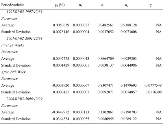
TABLE 6.2: Averages and standard deviations of GARCH parameters for three periods Period/variable μt (%) α0 α1 α2 γ 1997/01/02-1997/12/31 Parameter Average 0.0050639 0.0000027 0.0482561 0.9188128 NA Standard Deviation 0.0078146 0.0000004 0.0037652 0.0073608 NA 2001/01/02-2001/12/31 First 28 Weeks Parameter Average -0.0007775 0.0000043 0.8664709 0.0939303 NA Standard Deviation 0.0001429 0.0000001 0.0038137 0.0044986 NA After 29th Week Parameter Average -0.0003920 0.0000067 0.8307471 0.1479693 -0.0777548 Standard Deviation 0.0000425 0.0000007 0.0092871 0.0074857 0.0116308 2006/01/03-2006/12/29 Parameter Average -0.0447972 0.0000113 0.1302861 0.8190703 NA Standard Deviation 0.0364354 0.0000055 0.0080955 0.0289122 NA

CHAPTER 6. EMPIRICAL RESULTS 33 We proceed to estimate the unrestricted distribution parameters of futures returns. Since futures prices are censored by price limits, we need to overcome the effects of censoring in the data. In order to do this, the GARCH based algorithm of Morgan and Trevor (1999) is used and MATLAB is employed to apply their algorithm to obtain weekly estimates of unrestricted GARCH parameters as well as volatilities of each period. The averages of parameter estimates and the standard deviations of the unrestricted estimations of each period are summarized in Table 6.2. In all the three periods the GARCH parameters are statistically significant, whereas leverage term is significant for the second period starting from the 29th week.

6.3. Determining Optimal Margins and Price Limits with Various Tolerable Default Probabilities

The optimal margins and price limits are determined by solving8 our model in equations (12) to (19) and using the unrestricted distribution parameters. According to our model the exchange has to decide about the tolerable probability of default level. In an attempt to observe the impact of the chosen probability on optimal margins and price limits, the model is solved for the last day of each period under different probability levels ranging from 0.5% to 2.5%. In period 2, after 29th week we calculate different optimal margins for long and short positions and price limits for up and down moves due to the detected asymmetry. Figures 6.3.1, 6.3.2, 6.3.3 and 6.3.4 are the results of this exercise. As seen from the figures, when the tolerable probability increases, the margins and the price limits decrease as expected. Moreover, the difference between margin and price limit widens with increasing probability.

8 _{We use MATLAB’s fmincon nonlinear optimization function by assigning initial value 8 for both}

CHAPTER 6. EMPIRICAL RESULTS 34 Bold lines in each figure represent the actual margins imposed by the exchange on the chosen date. In period 1 the margin imposed by the exchange corresponds to a tolerable probability default level of 0.15% in either up or down moves. In periods 2 and 3 the actual margins used by the exchange corresponds to a tolerable probability level of more then 2.5% in both directions.

Margin and Price Limit for Given Probabilities (Period 1)

5.500 6.000 6.500 7.000 7.500 8.000 8.500 9.000 9.500 10.000 10.500 11.000 11.500 12.000 12.500 13.000 13.500 14.000 14.500 15.000 15.500 16.000 0. 05 % 0. 15 % 0. 25 % 0. 35 % 0. 45 % 0. 55 % 0. 65 % 0. 75 % 0. 85 % 0. 95 % 1. 05 % 1. 15 % 1. 25 % 1. 35 % 1. 45 % 1. 55 % 1. 65 % 1. 75 % 1. 85 % 1. 95 % 2. 05 % 2. 15 % 2. 25 % 2. 35 % 2. 45 %

Probability Of Exceeding Price Limit

Va lu e Margin Price Limit Actual Level

FIGURE 6.3.1: The relationship between tolerable probability and margin; tolerable probability and price limit for the last day of period 1

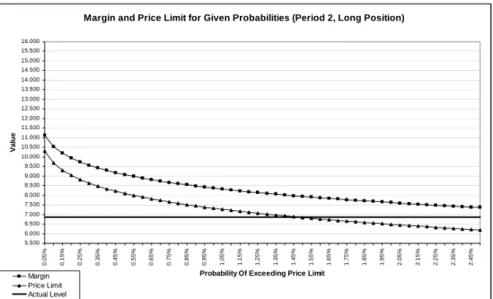
We would like to note that when asymmetry is detected in the data it might be important to estimate the volatilities with an asymmetric model as this could lead to very different optimal margin levels at each probability level for long and short positions as can be observed from our last day plots of period 2 (Figures 6.3.2 and 6.3.3).

CHAPTER 6. EMPIRICAL RESULTS 35

Margin and Price Limit for Given Probabilities (Period 2, Long Position)

5.500 6.000 6.500 7.000 7.500 8.000 8.500 9.000 9.500 10.000 10.500 11.000 11.500 12.000 12.500 13.000 13.500 14.000 14.500 15.000 15.500 16.000 0. 05% 0. 15% 0. 25% 0. 35% 0. 45% 0. 55% 0. 65% 0. 75% 0. 85% 0. 95% 1. 05% 1. 15% 1. 25% 1. 35% 1. 45% 1. 55% 1. 65% 1. 75% 1. 85% 1. 95% 2. 05% 2. 15% 2. 25% 2. 35% 2. 45%

Probability Of Exceeding Price Limit

Va lu e Margin Price Limit Actual Level

FIGURE 6.3.2: The relationship between tolerable probability and margin of long position; tolerable probability and lower price limit for the last day of period 2

Margin and Price Limit for Given Probabilities (Period 2, Short Position)

5.500 6.000 6.500 7.000 7.500 8.000 8.500 9.000 9.500 10.000 10.500 11.000 11.500 12.000 12.500 13.000 13.500 14.000 14.500 15.000 15.500 16.000 0. 05% 0. 15% 0. 25% 0. 35% 0. 45% 0. 55% 0. 65% 0. 75% 0. 85% 0. 95% 1. 05% 1. 15% 1. 25% 1. 35% 1. 45% 1. 55% 1. 65% 1. 75% 1. 85% 1. 95% 2. 05% 2. 15% 2. 25% 2. 35% 2. 45%

Probability Of Exceeding Price Limit

Va lu e Margin Price Limit Actual Level

CHAPTER 6. EMPIRICAL RESULTS 36 FIGURE 6.3.3: The relationship between tolerable probability and margin of short position; tolerable probability and lower price limit for the last day of period 2

Margin and Price Limit for Given Probabilities (Period 3)

5.500 6.000 6.500 7.000 7.500 8.000 8.500 9.000 9.500 10.000 10.500 11.000 11.500 12.000 12.500 13.000 13.500 14.000 14.500 15.000 15.500 16.000 0. 0 5% 0. 1 5% 0. 2 5% 0. 3 5% 0. 4 5% 0. 5 5% 0. 6 5% 0. 7 5% 0. 8 5% 0. 9 5% 1. 0 5% 1. 1 5% 1. 2 5% 1. 3 5% 1. 4 5% 1. 5 5% 1. 6 5% 1. 7 5% 1. 8 5% 1. 9 5% 2. 0 5% 2. 1 5% 2. 2 5% 2. 3 5% 2. 4 5%

Probability Of Exceeding Price Limit

Va lu e Margin Price Limit Actual Level

FIGURE 6.3.4: The relationship between tolerable probability and margin; tolerable probability and price limit for the last day of period 3

6.4. Weekly Optimal Margins and Price Limits with Chosen Tolerable Default Probabilities

The determination of the margins and price limits heavily depends on the chosen probability. Instead of imposing a pre-determined default probability, we compute and obtain the results for tolerable probability levels of 0.5% and 2.5% in one direction. Average weekly margins and price limits of each period are presented in Table 6.4.1.

CHAPTER 6. EMPIRICAL RESULTS 37

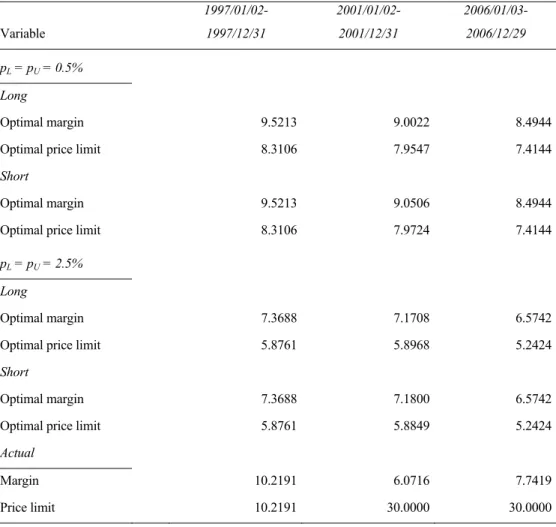
TABLE 6.4.1: Averages of actual and optimum margins and price limits of canola futures contract with tolerable probabilities of 0.5% and 2.5%

Variable 1997/01/02-1997/12/31 2001/01/02-2001/12/31 2006/01/03-2006/12/29 pL = pU = 0.5% Long Optimal margin 9.5213 9.0022 8.4944

Optimal price limit 8.3106 7.9547 7.4144

Short

Optimal margin 9.5213 9.0506 8.4944

Optimal price limit 8.3106 7.9724 7.4144

pL = pU = 2.5%

Long

Optimal margin 7.3688 7.1708 6.5742

Optimal price limit 5.8761 5.8968 5.2424

Short

Optimal margin 7.3688 7.1800 6.5742

Optimal price limit 5.8761 5.8849 5.2424

Actual

Margin 10.2191 6.0716 7.7419

Price limit 10.2191 30.0000 30.0000

CHAPTER 6. EMPIRICAL RESULTS 38 The average margins and price limits for tolerable probability levels of 0.5% and 2.5% in period 1 are lower then actual levels used by the exchange. In period 1 exchange uses a conservative margin which leads to high costs in terms of opportunity and liquidity. On the other hand, in period 2 optimal margins generated by our model are higher then actual margins. Although there exists a significant asymmetry between up and down movements after the 29th week of period 2 as discussed before, average margins of long and short positions are not quite different from each other. One reason behind this is that margins for long and short positions are the same for the first 28 weeks of period 2, because no asymmetry is observed in that part of the period. In an attempt to further investigate the other reason we calculate the differences of weekly margins between long and short positions for after the 29th week of period 2 with two tolerable probabilities (Figures 6.4.1 and 6.4.2). As can be observed from the figure in some weeks margins of short position are higher,

Margin Differences Between Short and Long Positions (p=0.5%)

-6.00 -4.00 -2.00 0.00 2.00 4.00 6.00 1 2 3 4 5 6 7 8 9 10 11 12 13 14 15 16 17 18 19 20 21 22 23 24 25 Weeks D if fer e n ce ( $/ to n n e) 0.5% Margin Difference

FIGURE 6.4.1: Optimal weekly margin differences between long and short positions after the 29th week of period 2 with tolerable probability of 0.5%

CHAPTER 6. EMPIRICAL RESULTS 39 and at some weeks lower than margins of long position. At some weeks the difference is very small like in weeks 19 ($-0.06) and 22 ($-0.23). These results also leads us to the fact that asymmetry in a futures contract return series may not always result in significant differences between margins. In period 3 average margins imposed by the exchange lies between average optimal margins with tolerable probabilities 0.5% and 2.5%. Price limits in the last years of periods 2 and 3 are 30 $/tonne, which are far more then margins, and therefore canola futures contracts in these periods are not self-enforcing.

Margin Differences Between Short and Long Positions (p=2.5%)

-6.00 -4.00 -2.00 0.00 2.00 4.00 6.00 1 2 3 4 5 6 7 8 9 10 11 12 13 14 15 16 17 18 19 20 21 22 23 24 25 Weeks D if fer e n ce ( $/ to n n e) 2.5% Margin Difference

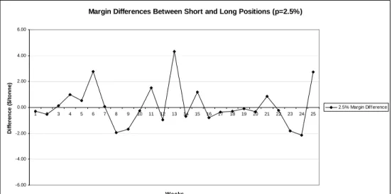
FIGURE 6.4.2: Optimal weekly margin differences between long and short positions after the 29th week of period 2 with tolerable probability of 2.5%

After determining weekly optimal margins for long and short positions, we compute how much more or less a trader pays as margin by comparing our results with actual levels. In order to make a comparison we assume that the trader is either long or short in the canola futures contract and keeps his position for one year by switching it with the nearby contract on the last day

CHAPTER 6. EMPIRICAL RESULTS 40 before the delivery month. Results are summarized in Table 6.4.2. In period 1, less margins would be paid by each trader in short and long positions if margins were set according to our model. On the other hand in period 2, since actual margin levels imposed by the exchange are lower than our optimal margins, traders in long and short positions would pay more compared to actual margins. As discussed above, the effect of asymmetry can be also seen in this table by observing that excess margins paid by the traders in long and short positions are different from each other. In addition, in period 3, if default probability of 2.5% was applied by the exchange traders would pay less

TABLE 6.4.2: Averages of excess margins that would be paid by the traders if our optimal margins were applied by the exchange for three periods

Variable 1997/01/02-1997/12/31 2001/01/02-2001/12/31 2006/01/03-2006/12/29 pL = pU = 0.5% Long

Total excess margin paid($/tonne) 174.67 -727.71 -165.19

Average daily excess margin paid($/tonne) 0.70 -2.92 -0.67

Short

Total excess margin paid($/tonne) 174.67 -739.76 -165.19

Average daily excess margin paid($/tonne) 0.70 -2.97 -0.67

pL = pU = 2.5%

Long

Total excess margin paid($/tonne) 712.79 -271.70 306.18

Average daily excess margin paid($/tonne) 2.85 -1.09 1.23

Short

Total excess margin paid($/tonne) 712.79 -273.99 306.18

Average daily excess margin paid($/tonne) 2.85 -1.10 1.23

CHAPTER 6. EMPIRICAL RESULTS 41

whereas if default probability of 0.5% was applied they would pay more then the actual margins.

6.5. Comparison of the Model with Price Limits and the Model in the Absence of Price Limits

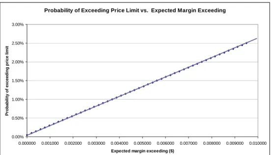
In the model with price limits determination of the margins and price limits heavily depends on the chosen probability whereas it is acceptable expected loss that determines margins and price limits in the model with no price limits. It is no possible to make an exact comparison between the two models, since one is valid when price limits are applied by the exchange and the other is valid in the absence of price limits. Therefore we compare the main determinants of these two models, which are acceptable default probability in the model with price limits and acceptable loss in the model without price limits. The relationship between them is presented in Figure 6.5 below.

As seen from the figure, there is a linear relationship between the tolerable probability level and the acceptable expected loss.