С І Ш У І■і Wii.T J .> й л dal ιί.. уѵ/ -Цч :«..| V d ¡г і WVл·; .!'**і ¿ W übtÍ ^ »... ¿\·
8
·ι Г.^'¡і и f .bVè Ί ■■‘'■i Ч ; f •'^.y 'ίΛ *«.. ·«,· ^ .«t» »iti»· · * .^'»v •t¿* ' i j ¿ 's í ‘tí .t,«« Vk»>' d « >a< --.· W'l» -SK^’ li-·' ; ·ν j r;.::; Jbü^VSRSiTY . . t w ¡ J { , J3
. d 4 fFUZZY CONTROLLER DESIGN FOR PARAMETRIC
CONTROLLERS
A THESIS
SUBMITTED TO THE DEPARTMENT OF ELECTRICAL AND
ELECTRONICS ENGINEERING
AND THE INSTITUTE OF ENGINEERING AND SCIENCES
OF BILKENT UNIVERSITY
IN PARTIAL FULFILLMENT OF THE REQUIREMENTS
FOR THE DEGREE OF
MASTER OF SCIENCE
By
Murat Akgiil September 1996
Q f t
. f t İ U \9д^=
I certify that I have read this thesis and that in my opinion it is fully adequate, in scope and in quality, as a thesis for the degree of Master of Science.
ler Morgül(Supervisor)
I certify that I have read this thesis and that in my opinion it is fully adequate, in scope and in quality, as a thesis for the degree of Master of Science.
Prof. Dr. M. Erol Sezer
I certify that I have read this thesis and that in my opinion it is fully adequate, in scope and in quality, as a thesis for the degree of Master of Science.
Assoc. Prof. Dr. M. Ir§aai Aksun
Approved for the Institute of Engineering and Sciences:
Prof. Dr. Mehmet®iaray
Director of Institute of Engineering and Sciences
ABSTRACT
FUZZY CONTROLLER DESIGN FOR PARAMETRIC
CONTROLLERS
Murat Akgiil
M .S. in Electrical and Electronics Engineering Supervisor; Assoc. Prof. Dr. Omer Morgiil
September 1996
In this thesis, fuzzy logic controller (FLC) design for tuning some parametric controller is investigated. The objective in designing an FLC is to determine the rule bcise of the system and the data base which includes membership functions, set operations, and inference engine. Two designs have been realized using heuristic rule generation; one for a PID controller and one for a lead-lag type controller. The FTCs in these designs set the parcimeters of the PID and lead- lag controller on-line. The rules and the corresponding membership functions are constructed by observing the effect of the changes of the parameters on the overall performance. One other design is performed using the desired input- output data pairs. In this design Fuzzy c-Means clustering algorithm is used to e.xtract the rules and the membership functions from the input-output data of the system. Simulation results showed that better controller performance can be cichieved by FLCs in comparison with the classical design methods.
Keywords : Fuzzy logic, fuzzy logic controllers, fuzzy c-means clustering algorithm, membership function.
ÖZET
P A R A M E T R I K D E N E T L E Y İC İL E R İÇİN B U L A N IK D E N E T L E Y İC İ T A S A R L A N M A S I
Murat Akgül
Elektrik ve Elektronik Mühendisliği Bölümü Yüksek Lisans Tez Yöneticisi; Assoc. Prof. Dr. Ömer Morgül
Eylül 1996
Bu tezde, parametrik denetleyicilerin ayarlanması için bulanık mantığa dayalı denetleyici (BM DD) tasarımı incelenmiştir. Bulanık mantığa dayalı denetleyici tasarımında amaç, sistemin kural tabanını ve içinde üyelik fonksiyonlarının, küme işlemlerinin, ve çıkarım mekanizmasının bulunduğu veri tabanının be lirlenmesidir. Biri PID diğeri faz kaydırmak denetleyici için sezgiye dayalı iki tasarım gerçekleştirilmiştir. Bu tasarımdaki BMDD’ler PID ve faz kaydırtılalı denetleyicilerin parametrelerini eş zamanlı olarak belirlemektedir. Kurallar ve onlara bağlı üyelik fonksiyonları, bu parametre değişimlerinin bütün sistemin performansına etkisi gözlenerek oluşturulmuştur. Bir başka tasarım da sis teme ait istenen giriş ve çıkış sinyalleri kullanılarak gerçekleştirilmiştir. Bu tasarımda, Bulanık c-Ortalamalı kümeleme algoritması, kuralların ve üyelik fonksiyonların eldeki giriş ve çıkış sinyallerinden çıkartılmasında kullanılmıştır. Simulasyon sonuçları, BM DD’ ler ile klasik tasarım metodlarına göre daha iyi bir performansa ulaşılabileceğini göstermiştir.
Anahtar kelimeler : Bulanık mantık, bulanık mantık denetleyiciler, bulanık c-ortalarnalı kümeleme algoritması, üyelik fonksiyonu.
ACKNOWLEDGMENTS
I would like to express my deep gratitude to my supervisor Assoc. Prof. Dr. Omer Morgiil for their guidance, suggestions, and invaluable encouragement throughout the development of this thesis. I would like to thank to Prof. Dr. M. Erol Sezer and Assoc. Prof. Dr. M. Ir§adi Aksun for reading and commenting on the thesis.
.And special thanks to all Graduate Students in this department for their continuous support.
TABLE OF CONTENTS
1 INTRODUCTION
1
2 Mathematical Preliminaries 42.1
Fuzzy S e t s ...4
2.2
Operations On Fuzzy S e t s ...,5
2.3 Fuzzy R elation s...6
2.4 Implication10
3 F U Z Z Y CO N TR O L 12 3.1 The Control P r o b le m ...12
3.2
Classification Of Fuzzy Logic Systems... 133
.2.1
Pure F L S ... 133
.2.2
Takagi and Sugeno’s F L S ... 143.2.3 FLS with Fuzzifier and Defuzzifier... 14
3.3 Computational Structure of FLS with Fuzzifier and Defuzzifier . 15 3.3.1 Fuzzification... 17
3
.3.2
Rule F i r i n g ... 19 vi3.3.3 Defuzzification
20
3.4 Design of Fuzzy Logic Controller
20
3.4.1 Derivation of R u le s ... 22
4 Fiizzy Logic Controller Design : Heuristic Rule Generation 24
4.1 PID Controller D e s ig n ... 24
4.1.1 Rule-Base Construction 25
4.1.2 FLC Structure 28
4.1.3 Simulations and R e s u lt s ... 29
4.2
Lead-Lag Controller Design34
4.2.1 Rule-Base Construction
34
4.2.2 FLC Structure
37
4.2.3 Simulations and R e s u lt s ... 37
5 Fuzzy Controller Design : Rule generation using fuzzy c-means
clustering algorithm 40
5.1 Dynamic Programming... 43
5.2
Fuzzy C-Means Clustering A lg o rith m ... 445.3 Formation of Membership Functions 46
5.4 Simulations and R e s u lt s ... 47
6 Conclusion 51
LIST OF FIGURES
3.1 System structure under investigation
12
3.2 Basic configuration of pure F L S ... 14 3.3 Basic configuration of Takagi and Sugeno’s F L S ... 14 3.4 FLS with fuzzifier and d e fu z z ifie r ... 15 3.5 Computational Structure of FLS with fuzzifier and defuzzifier . 15
3.6 Membership functions 18
3.7 Clipped fuzzy sets as a result of rule f i r i n g ... 19
4.1 System structure under in v estig a tion ... 25 4.2 A typical step response of a system... 26 4.3 Membership functions for error and increment of error 28 4.4 Membership function for the variables 7\p, Ki, and K,i 29 4.5 Membership function for the variables 7\p, 7C,, and A'j ...31 4.6 Comparison of the step responses... 32 4.7 PID parameters determined by the FLCs... 32
4.8 Comparison of the step responses.
3.3
4.9 PID parameters determined by the FLCs.
33
4.10 System structure under investigation
34
4.11 Step responses of Pi(s) for a=0.01, 0.3.
0
.7
.1
,2
,0
, 10.35
4.12 Step respon.ses of ^2
(3
) for a=0.01, 0.3. 0.7, 1, 2, 3, 4. 35 4.13 Membership functions of the linguistic variable a 36 4.14 Comparison of the step responses of /^}(s) with the two differentcontroller... 38 4.15 (a) Step responses of P4{s). (b) Variation of the parametera. 39
5.1 The membership functions and the relation of the rule if “e is LE,^ then “ u is LUE.
5.5 The suboptimum solution for the proportional control and the corresponding step response.
5.6
Rule base of the fuzzy controller5.7 (a) The step responses with two different controller (b) The waveform for the proportional gain.
5.8 (a) The step responses with two different controller for the sys tem with disturbed parameter (b) The waveform for the propor tional gain.
41
5.2
Negative unit feedback with a parametric controller C(s,p) . . . 41 5.3 Sample point of error versus the corresponding control signal. 42 5.4 Negative unit feedback with a proportional controller K 4747 49
50
50
C hapter 1
I N T R O D U C T I O N
Over the past few years many researchers of various fields and manufacturers of control equipment pay a great attention to fuzzy control. There are still however, two predominant extreme positions as to the benefits of fuzzy con trol. On the one hand, many proponents of this technology claim that fuzzy control will revolutionize control engineering, promises major breakthroughs, and will be able to solve complex engineering problems with very little effort. On the other hand, many representatives of the control engineering community still proclaim that “everything that can be done in fuzzy control can be done conventionally as well” and announce a breakdown of the “fuzzy hype” in the near future.
A fuzzy control system is a real time expert system implementing a part of a human operator’s or process engineer’s expertise which does not lend itself to being easily expressed in PID-parameters of differential equation but rather in situation/action rules. However, fuzzy control differs from main-stream expert system technology in several aspects. One main feature of fuzzy control systems is that there are symbolic if-then rules and qualitative, fuzzy variables and values such as
if “ pressure is high” and “slightly increasing” then “energy supply is negative medium”
Most of the inventors of fuzzy control have a strong control engineering and systems theory background. From their perspective, fuzzy control can be seen as heuristic and modular way for defining nonlinear, table based systems. Reconsider the rule above : it is nothing but an informal '■‘nonlinear PD- elernent” .
A representation theorem, mainly due to Kosko d], states that any contin uous nonlinear function can be approximated as closely as needed with a finite set of fuzzy variables, values, and rules. This theorem describes the representa tional power of fuzzy control in principle, but it does not answer the questions of how many rules are needed and how they can be found, which are of course essential to real-world problems and solutions.
It is generally agreed that ciri important point in the evolution of the mod ern concept of uncertainty was the publication of a seminal paper by Lofti .A. Zadeh [1965], even though some ideas presented in the paper were envisioned some 30 years earlier by the American philosopher Max Black [1937]. In his paper, Zadeh introduced a theory whose oh]ecis-fuzzy seis-are sets with bound aries that are not precise. The membership in a fuzzy set is not a matter of affirmation or denial, but rather a matter of degree.
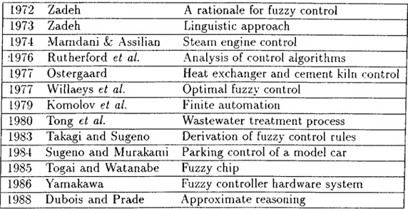
The literature in fuzzy control has been growing rapidly in recent years, making it difficult to present a comprehensive survey of the wide variety of applications that have been made. Historically, the important milestones in the development of fuzzy control may be summarized as shown in Table.
1.1
[‘2].The first successful industrial application of the FLC was a cement kiln con trol system developed by the Danish cement plant manufacturer F. L. Smidth in 1979.
Fuzzy Logic Controllers(F'LCs) can be used in various ways. One of them is to use the FLC directly as the controller for the system under consideration. The other choice is to use a standard controller like PID or lead-lag and tune the parameters of this controller with a fuzzy logic system (FLS). A few of the studies on parameter tunings are [3], [4] and [5]. In [4] the PID parameters are tuned according to some rules derived by considering a typical system output. In [
5
] some changes to the model of fuzzy PI controller is introduced to reduce1972 Zadeh A rationale for fuzzy control
1973 Zadeh Linguistic approach
1974 Mamdani &: Assilian Steam engine control
.4976 Rutherford et al. Analysis of control algorithms
1977 Ostergaard Heat exchanger and cement kiln control 1977 VVillaeys et ai Optimal fuzzy control
1979 Komolov et al. Finite automation
1980 Tong et al. Wastewater treatment process 1983 Takagi and Sugeno Derivation of fuzzy control rules 1984 Sugeno and Murakami Parking control of a model car 1985 Togai and Watanabe Fuzzy chip
1986 Yamakawa Fuzzy controller hardware system 1988 Dubois and Prade Approximate reasoning
Table
1
.1
: Some important studies in fuzzy control. the overshoot even more.In this thesis the implementation of a fuzzy controller which sets the pa rameters of a parametric controller has been investigated. .Vlainly two different methods have been used in constructing the rule base. In the first method we obtain the rules by observing the input output data of the system. Here we obtain the fuzzy rules to set the parameters of the parametric controller heuris- tically. For the controller, we consider the standard PID, and the lead-lag type controllers. In the other part again the input-output data is used but this time the rules have been set from the results of Fuzzy C-.Means (FCM) clustering algorithm.
In Chapter
2
some definitions and the mathematical preliminaries to fuzzy operations on fuzzy sets are given. In Chapter .3 an introduction to fuzzy control is given and various ways to find the required rules are explained. In the remaining chapters fuzzy controller design for PID and lead-lag type controllers are investigated. In Chapter 4 the rule generation is done heuristically and in Chapter 5 this is performed by Fuzzy C-Means(FCM) clustering algorithm. Finally in Chapter6
we give some concluding remarks.Chapter 2
M athem atical Preliminaries
2.1
Fuzzy Sets
A classical set is a collection of objects of any kind. Let X be the universe of discourse on which the set A is defined. There are several ways to decide if an element x belongs to the set A or not. One way is to use a characteristic function.
D efin ition
1
f.ij( : X — > {0
,1
} is a characttristic function o f the set A iff 1 , x e AVx G X, ¡.lA - '
0
,x ^ A .□
The characteristic function ha takes values
1
and 0 depending on whether an elements belongs to the set A or not. This is due to the lack of ambiguity in the definition of set A. Let H be a set defined as “numbers close to1
.5
” . Here the closeness in the definition is not clear. Due to this vagueness the set B can not have sharp borders as the set A has. Therefore one can not use the codomain {0
,1
} of the characteristic function, instead for any element x a grade of membership value in the interval [0,1] must be assigned. After this motivation the definition of fuzzy set can be done as follows;D efin ition
2
The membership function ¡.ijr o f a fuzzy set T is a function /ijT ; U — »■ [0,1]. -F is completely determined by the set o f tuplesLet us reconsider the fuzzy set B, “numbers close to
1
.5
” . This fuzzy set can be represented with the following set of tuples ;B = { (
0
.0
,0
.0
), (0
.2
,0.5), (0.5,1.0), (1
.0
,1.5). (0.5,2
.0
), (0
.2
,2.5), (0
.0
,3
.0
)}. Here the first entry of the tuples is the grade of membership of the second entry, u. These tuples are also given with the following representation:B = 10.0/0.0,0.2/0.5,0.5/1.0,1.0/1.5,0.5/2.0,0.2/2.5,0.0/3.0}.
The division symbol, in the above notation, does not mean to divide the membership grade to the value of the element u, it is just used to represent the pairs.
2.2
Operations On Fuzzy Sets
In classical set theory, the union, intersection and complement of sets are simple operations that are unambiguously defined. The unambiguity follows from the fact that logical operators AND, OR, and NOT have a well defined semantics based on propositional logic. For example, “'A AND B ” in propositional logic is true if and only if both expressions A and B are true. In fuzzy set theory their interpretation is not so simple, because graded characteristic functions (membership function ) are used. Zadeh proposed [
6
] the following definitions for the union, intersection and complement operations on fuzzy sets.D efin ition
3
Let A and B be two fuzzy sets and let /i^(·) and //s(·) be their membership functions, respectively. Then the membership function o f the setsA U B . may he given as follows :
' i x e X :
/UnB(x) = min(//^(x)./zs(x)),
W x e X : yu^us(x) = rnax(//^(x).;£e(x)),
V x e X : /£^c(x) =
1
- ^m(x). □If the values of and i-Cb{x) are restricted to the set {0,
1
} then the results reduce to the classical set operations. Therefore this is a very simple extension of the classical operations. There are other extensions, for example,Vi € X : /Uns(-c) = /£^(i) · /ie(x),
Vi e X : H A u B i x ) = min(l.^i^(i) + /Z£?(i)).
In comparison with the lattice (min and max) operations, here the degree of membership depends on both the values of membership function yu^(i) and ytis(i). In our studies the operations proposed by Zadeh was used. A list of other operations can be found in [2], [7] and [
8
].Among these operations, t-norm and t-conorm( sometimes referred as s- norm) take many researchers interest. These logical connectives posses some properties like boundary conditions, commutativity, associativity. The bound ary conditions indicate that the logical connectives for fuzzy sets coincide with those applied in two valued logic. The property of commutativity reflects a case in which the truth value of a composite expression does not depend on the or der of the components used in its formation. These concepts are explained in [
7
] and [8
] in more detail with examples.2.3
Fuzzy Relations
A relation can be considered as a set of tuples, where a tuple is an ordered pair. A binary tuple is denoted as (a:, y), and in general an n-ary tuple is { x i , ^
2
, ···, a^n)· Just like classical sets, classical relations can be described by a characteristic function as well.D efin ition 4 ^-¡i : X\ x X2 x ■ ■ ■ x — > {
0
,1
} is a characteristic function o f the set R iffV(xi, X
2
, x „ ) e A'l X A2
X ■ ■ · X A'„, = < 1 ,(X i.X2
,...,Xa) G 0 ,(X i.X2
,...,Xa) ^ 7?.. □ In a fuzzy relation this characteristic function is extended to the interval [0,1
]. A fuzzy relation is a fuzzy set of tuples, i.e. each tuple has a membership degree between0
and1
.D efin ition 5 Let U and V be uncountable (continuous) universes and ¡.1% :
U x Then
J u x V
is a binary relation on U x V. If U and V are co untable (discrete) un iverses, then we can take
H v )/(u , v). □
U x V
In this notation the division is used to represent the pairs of an element and its membership grade of the corresponding fuzzy set. The integral and the summation symbols do not mean the well known algebraic integration over an argument or taking the sum of all the pairs. They are used to combine all the pairs which constitute the set R. In this thesis only the discrete universes are studied. Therefore from now on, only the second part of the definition will be used.
Fuzzy relations are very important in fuzzy control because they can de scribe interactions between variables. Union, intersection and complement op erations can be defined in any way as was described in the previous section. Apart from these operations there are two very important operations on fuzzy sets and fuzzy relation, namely projection and cylindrical extension.
D efin ition
6
Let U and V be two independent domain. And let TZ be a fuzzy relation on U x V. Then the projection of 71 on V is defined byp r o j l l o n V ^ Y ] max ^ivefxi. . . x „ ) / ( x , x . J . D V
*■ '1
... ■’‘■'iE x a m p le : Let X and Y be two independent domains such that a relation IZ is defined on X x Y. Assume that the relation IZ is defined as “x is considerable larger than y ” . Then this relation may be given by the following array :
TZ V2 V3
1/4
Xi
0.8
l.O0.1
0.7 2*20.0 0.8 0.0 0.0
X3
0.91.0
0.70.8
Then the projection of 7^ on X means that a:, is assigned the highest member ship degree from the tuples (a·,, yj), j = l,...,4 for i= l,...,3 . So,
proj 7?. on X = 1.0/ari + O.
8
/X2
+ l-O/ja,proj TZ on Y = 0.9/j/i + l.O/i
/2
T0
-7
/y3
-f- 0.8
/2
/4
.D efin ition 7 Let S be a fuzzy set defined on V, and let U be a domain in dependent o f V. Then the cylindrical extension o f S into U is a relation on U y. V defined as:
u
, where k and n are the dimensions o f the domains V and UxV, respectively.
□
E x a m p le : Consider the fuzzy sets A and B given below
A — proj 7?. on X =
1
.0
/ari + O.8
/X2
+ l-O/x^,So the cylindrical extension of A into Y and the cylindrical extension of B into X are given as follows :
ce(.4) Xl
•^2
y\1.0
0.8
l.O i/2
1.0 0.81.0
y-i1.0
0.81.0
i/41.0
0.8
1.0
ce(B) yi y-i y-i i/i 0.9
1.0
0.70.8
X2 0.91.0
0.70.8
^3 0.9 l.O 0.70.8
Having defined cylindrical extension, one can calculate the intersection of a set >1 on X and a relation 7^ on X x Y by first taking the cylindrical extension of A into Y and taking the minimum of the associated elements of the two fuzzy sets, ce(>l) and TZ, where both are defined on X x Y.
The combination of a fuzzy set and a fuzzy relation with the aid of cylin drical e.xtension and projection is called a composition. It is denoted by the symbol “o’’ . A fuzzy relation, as its name indicates, is a relation between its subsets. This operation is necessary when one knows the relation of a certain subject and some related facts and wants to calculate the facts which he does not know.
Definition
8
Let A be a fuzzy set defined on A’ and 71 be a fuzzy relation defined on X x Y. Then the composition o f A and 71 resulting in a fuzzy set B defined on Y is given byB = AoTZ = proj ( ce(.4) DlZ ) on Y .O
Example : Consider a relation defined as “x is approximately equal to y ” , TZ, defined on X x Y and suppose it is known that “x is small” is expressed by a fuzzy set A on X. Let the fuzzy relation 1Z, and the fuzzy set A be given as follows. TZ yi y2 ys Xl
1.0 0.8
0.3 X20.8 1.0 0.8
xz 0.30.8 1.0
A =0
.2
/x i -I 1.0/a:2 +0
.8
/0
:3
.Then the cylindrical extension of
A
into Y is, ce{A ) !Ji V2 ;!/3XX
0.2 0.2 0.2
X21.0
l.O1.0
^3 I0.8 0.8 0.8
So the intersection of ce(v4) and 7Z, calculated with the ininirnum operator, results in the following relation :
ce(A ) n TZ Vi V2 y-i
Xi
0.2 0.2 0.2
^2
0.8 1.0 0.8
0
.:j0.8 0.8
And finally taking the projection into Y resultsB = 0.8/t/i + l-O/j
/2
+0
.8
/r/3
·The fuzzy set B can be characterized as “x is approximately equal to y ” AND ■‘x is small” or equivalently “y is more or less small” .
2.4 Implication
In classical logic the truth value of p q is defined as shown in the Table.2.1. This implication or if-then ( if p then q ) statement can be expressed with different combination of union, intersection and complement operations.
Some equivalent expressions would be -ipVq and {pAq)\/-<p where “V” , “A” and stand for union, intersection and complement operations, respectively. Here p and q can be considered as sets which are defined by a characteristic function whose domain is the set {0, 1}. To extend the implication operation into fuzzy domain again the codomain of the characteristic function of p and q must be extended to the closed unit interval, [
0
,1
], and instead of the classicalP q p =» q
0 0
1
0 1
1
1 0
0
1 l
1
Table
2
.1
: Truth table for p implies qset operations, their fuzzy counterparts must be used. Having done these, one can calculate the truth value of an if-then statement. A typical example which may be encountered in fuzzy control might be the following type of statement,
if “ pressure is rather high” then “energy supply is negative big” .
The classical set operators p ^ q, -■pVq, and (p A</) V ->p, have all the same truth table. When these operators are replaced with fuzzy operators, then the equivalent of p q may differ according to the selected union, intersection and complement operators. There are a number of relations that can be used to represent the meaning of an if-then statement. Some of these are equivalent to the logical implication p => q and some are not. In this study Mamdani implication defined below is used.
Suppose that there is an if-then statement as given below and it is desired to calculate the truth value of this implication.
if A then B.
Let A and B be two fuzzy proposition defined on X and Y, respectively. Assume that TZc be the relation defined with the above if-then statement, then the calculation related with the Mamdani implication is as follows.
Tic = ce(^ ) A ce{B),
= min(p^(x),/i£t(l/))·
There are other implication operations. An extended list of these can be found in [2], [7].
C hapter 3
F U Z Z Y C O N T R O L
3.1
The Control Problem
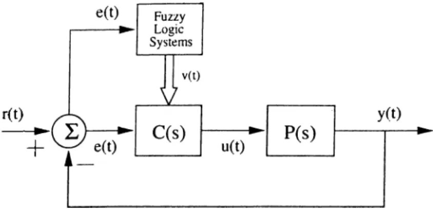
The control problem which we tried to investigate in this thesis is reference input tracking. The system structure under investigation is unit feedback with controller and linear systems which is shown in Fig.3.1
r(t) +
Figure 3.1: System structure under investigation
In this figure, C(s) is the transfer function of a parametric controller, P(s) is the transfer function of the plant under investigation, r(t) is the reference input, y(t) is the output of the system, u(t) is the output of the controller,
e(t)= r(t)-y(t) is the input of the controller and, v(t) is a vector function in representing the waveform for the parameters of the controller. Here w is the number of parameters that the controller C(s) has. These parameters are updated by the Fuzzy Logic Systern(FLS) according to the error signal. In this thesis the problem is investigated for the unit step reference signal.
The block Fuzzy Logic Systems in Fig.3.1 may be composed of more than one FLS, described in the following section. For each parameter of the con troller there is a corresponding FLS with its own rules and membership func tions.
3.2
Classification O f Fuzzy Logic Systems
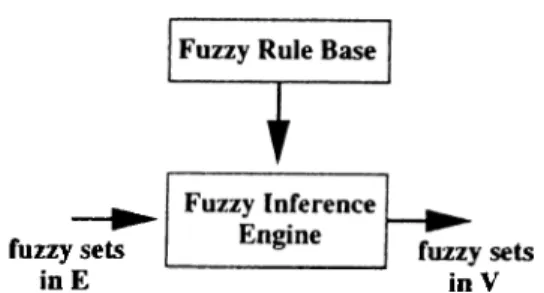
Fuzzy logic systems is a name for the systems which have a direct relationship with fuzzy concepts (like fuzzy sets, linguistic variables, and so on) and fuzzy logic. The most popular fuzzy logic systems in the literature may be classified into three types: pure fuzzy logic systems, Takagi and Sugeno’s fuzzy system, and fuzzy logic systems with fuzzifier and defuzzifier.
3.2.1
Pure FLS
The basic configuration for a pure FLS is shown in Fig.3.2, where the fuzzy rule base consists of a collection of fuzzy if-then rules, and the fuzzy inference engine uses these fuzzy if-then rules to determine a mapping from fuzzy sets in the input universe of discourse E C 3?'^ to fuzzy sets in the output universe of discourse V C S’)? based on fuzzy logic principles. The fuzzy if-then rules are of the following form:
111 : if xi is Fi AND · · · AND Xn is F ‘ THEN y is G‘ . (3.1) where F ‘ and G‘ are fuzzy sets, x = (a:i, ...,XnV G E and j/ G V are input and output linguistic variables, respectively, and / =
1
,2
, ...,M .fuzzy sets
in E
in V
Figure
3
.2
: Basic configuration of pure FLS3,2.2
Takagi and Sugeno’s FLS
instead of considering the fuzzy if-then rules in the form of Eqn.
3
.1
, Takagi and Sugeno proposed to use the following fuzzy if-then rules:Ki : if xi is F ‘ AND · · · AND is
THEN = Cq -p Cj X arj -p · · · -p x
Xn-(3.2)
where F- are fuzzy sets, C{ are real-valued parameters, y ‘ is the system output due to rule and / = 1,2,..., M .
Figure 3.3: Basic configuration of Takagi and Sugeno’s FLS
3.2.3
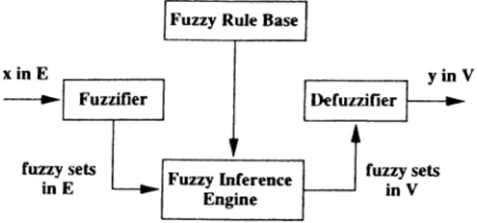
FLS with Fuzzifier and Defuzzifier
In order to use the pure FLS shown in Fig.3.2 in engineering systems where inputs and outputs are real-valued variables, the most straightforward way is to add a fuzzifier to the input and a defuzzifier to the output of the pure FLS.
The basic configuration of fuzzy logic system with fuzzifier and defuzzifier is shown in Fig.3.4 The fuzzifier maps real-valued inputs(crisp points) in E to luzzy sets in E, and the defuzzifier maps the fuzzy sets in V to real-valued control outputs(crisp points) in V.
In this thesis while designing a fuzzy controller, the structure of the fuzzy logic systems with tuzzifier and defuzzifier are used. The computational struc ture ot this type of system will be given in the next section. More detail for the other two types of fuzzy systems can be found in [
9
j.Figure 3.4: FLS with fuzzifier and defuzzifier
3.3
Computational Structure of FLS with
Fuzzifier and Defuzzifier
The computational structure of a FLS consists of a number of computational steps as presented in Fig.3.5. There are five such computational steps.
Figure 3.5: Computational Structure of FLS with fuzzifier and defuzzifier
A typical FLS has a number of rules. These rules for example can have the following form :
n , : if “ei is AND ... AND “ e,„ is THEN “ u is (3.3) where LE\^\ ..., LE\^'^ are the linguistic values taken by the process state vari ables) linguistic variables) e i,...,e ,„ in the rule-antecedent of the rule. The meaning of each linguistic value LE]^'^ is represented by a membership function defined on a domain, say, e of the process variable tk. Thus the meaning of LE]^^ is given by ¡.irrpis) : e — >· [0 ,
1
]. The objective is to find a value for the control variable v using a set of rules in the form of Eqn.3.3.The states of a system can be measured with some sensors. These sensors provide, for example, some voltage values like 1.23V which is a crisp value.
The range of these different sensors might be different and therefore the domain of the membership functions related with the propositions in the rules will be different. If all of these membership functions are defined on a com mon domain then the inputs(state values) must be scaled so that each will be mapped onto its physical input domain. Input Scaling is not needed when the definitions of the membership functions are made on the physical domain of the inputs.
So far, the described fuzzy calculations are made on fuzzy domain, that is the arguments of the fuzzy operators are all fuzzy sets. Therefore to use the measurement of the sensors, one hcis to convert these crisp values into fuzzy set. This is called fuzzification. The result of fuzzy calculations are again fuzzy sets. But the controller output must be a crisp value to drive the system. Therefore a defuzzification module is needed to convert the fuzzy set to a suitable crisp value.
In section Sec.
2
.4 the calculations of the relation corresponding to an if-then statement with Mamdani implication is given. Performing this calculation one can obtain the relation related with the rule, and with the composition operation given in Sec.2.3, the fuzzy set corresponding to the controller output can be calculated.These calculations can be performed for an FLS with a single rule in a straightforward way. For an FLS with multi-rule these calculations can be
performed in two different ways. One of them is the composition based inference and the other is the individual-rule based inference. These two methods result in the same fuzzy set for the controller output if Mamdani implication is used to represent the meaning of the rules. There e.xist some implication operations which result in different fuzzy sets for the two method of inference. One of these implications is Godel implication[7].
In composition based inference, first all the relations for each rule are cal culated. Then with a fuzzy union( OR ) operator, these relations are combined into a single relation representing the complete rule base. Then the composi tion of the fuzzified input and this overall relation results in the fuzzy set for the controller output. In other words,
U = p" 0% where, //* is the membership function after fuzzification of the input variables, e* = (et,...,em ),
n
"Rs is the relations corresponding to the rule. (3.4) An if-then rule is a relation between the corresponding domain of the propo sition in its antecedent and consequent parts. Rule firing is the process of obtaining the fuzzy set for the consequent proposition using the relation corre sponding to the if-then rule and the observed crisp input values. Rule firing is given in more detail in Sec.3.3.2. In individual-rule based inference, each rule is fired individually and a fuzzy set for the controller output is obtained. Then the union of these fuzzy sets gives the resultant fuzzy set for the controller output. Composition based inference of rules requires much more calculations than individual-rule based inference, therefore the second inference method is used to get the fuzzy set for the controller output.
3.3.1
Fuzzification
Fuzzification operation depends on the inference method used. For composition based inference, fuzzification of the input, e* = (ej,...,e)^) means a fuzzy set
having the membership function
¡
1*
which is defined as follows : I for Cl = = e;„0
otherwise.(3.5)
fo r the individual-rule based inference, the fuzzification operation means the following. The states of a system can be measured by some sensors. These sensors can provide, for example, some voltage values like 1.23Vfi which is a crisp value. In the rule-antecedent of the if-then statement there exists fuzzy propositions like “ cyt is It is known that = 1.23T and to perform fuzzy calculations related with the rules, it is required to have a truth value for the proposition “ca, is For this method of inieience fuzzification is
the process of finding the membership degree of el in .And this is done for every element of e* where e* = (e^,...,
Example : Consider the rules
Ri : if “ e is S M A L L ” THEN “ u is S M A L L ” , R2 : if “ e is B IG ” THEN “w is B I G ” .
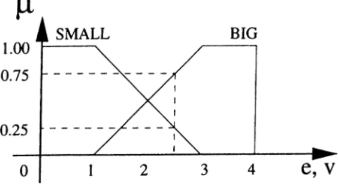
In Fig.3.6 the related membership functions for e and v are given. Let e* = 2.5. Then from Fig.3.6 we obtain the degrees of membership i-''S.\rALL('^-o) — 0.25. So the fuzzification of e’ = 2.5 for the first rule, Ri, means the membership value of tisMALL(‘2.5) = 0.25. Similarly the fuzzification of e* = 2.5 for the second rule, means the membership value of /as/g'(2-5) = 0.75
Figure 3.6: Membership functions
3.3.2
Rule Firing
Rule firing is to calculate a membership function for the proposition in the consequent part of the if-then statement. Let the rule be as in Eqn.3.3. Then with the fuzzification operation the truth values for the propositions ”e/t is is known. With a fuzzy AND operator the truth value of the antecedent part of the if-then statement can be calculated. The result of this calculation will be a crisp value since the inputs are crisp values. Ne.xt from Sec.
2
.4, one of the implication procedure is chosen. The fuzzy set for the control output is obtained by calculating the result of the implication operation for the calculated truth value of the antecedent part of the if-then statement with every control value. For Mamdani implication this fuzzy set will be calculated by the following ecjuation.Vu € V : ^icLv{v) = min(min(/i^^(u(ei),. . . , /i^K(v))· (3.6)
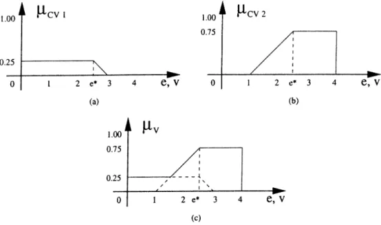
Example : Consider again the same if-then statements in the previous exam ple. The propositions has a truth value 0.25 for the first rule and 0.75 for the second rule. If we chose Mamdani implication for the inference engine then the firing of a rule means to clip the membership function given in the consequent part of the rule at the point of the truth value of the antecedent part.
Figure 3.7: Clipped fuzzy sets as a result of rule firing
Therefore firing the first rule will result a membership function for v as given in Fig.
3
.7
.a. For the second rule the membership function BIG will be clipped at point 0.75 as shown in Fig.3.7.b. To use all the information supplied by each one of the rules, we have to take the union of these clipped fuzzy sets. Choosing the union operator as the maximum operation we find the fuzzy set for the linguistic variable v as giv'en in Fig.3.7.c. This is the fuzzy set to which the defuzzification operation must be applied.3.3.3 Defuzzification
As explained previously the output of the inference process is a fuzzy set. in the on-line control, a non-fuzzy(crisp) control action is usually required. Consequently, one must defuzzify the control output inferred from the fuzzy control algorithm. There are many defuzzification methods proposed by many researchers[7],[
8
],[2],[9]. One of these method is center of gravity and used in the simulations of this thesis. This defuzzification method calculates the gravity point of the membership function ¡.ly with respect to the control variable vand sets the gravity center as the defuzzified control output.3.4
Design of Fuzzy Logic Controller
The design parameters of a fuzzy logic controller(FLC) can be summarized as follows:
Inference Method :
• Choice of inference method
Fuzzification Module :
• Choice of fuzzification method
Rule Base :
• Choice of Variables and Content of Rules • Choice of a Term Set
• Derivation of Rules
Data Base :
• Choice of Membership Functions • Choice of Scaling Factors
Defuzzification Module :
• Choice of defuzzification method
After choosing the method for the inference one also has made the choice for the fuzzification operation as explained in the previous section. Choice for the input and control variable is done according to the problem in hand. Typically, the linguistic variables in a FLS are the state, state error, derivative, state error integral, etc. There is no well established method for the choice of term set,which is the linguistic values like small, positive big, slightly increasing etc., membership function, scaling factors, and defuzzification method. Most of the time the choices are done by trial and error method. Therefore experience and engineering knowledge play an important role during this selection stage. There are some studies to determine these parameters from the input output data of the system [10], [11] and studies related with the effects of the variations of these parameters to the performance of the overall system [2], [7].
3.4.1
Derivation of Rules
There are five approaches for the derivation of fuzzv control rules.
Expert Experience and Control Engineering Knowledge: The formula tion of fuzzy control rules can be achieved by means of two heuristic approaches. The most common one involves an introspective verbalization of human exper tise. The other approach includes an interrogation of e.xperts or operators using a carefully organized questionnaire.
Based on Operator’s Control Actions: In many industrial man-machine control systems, the input-output relations are not known with sufficient pre cision to make it possible to employ classical control theory for modeling and simulation. And yet skilled human operators can control such systems quite successfully without having any quantitative models in mind. In effect, a hu man operator employs, consciously or subconsciously, a set of fuzzy if-then rules to control the process. In practice, such rules can be deduced from the observation of human controller’s actions in terms of the input-output data. Based on the Fuzzy M odel of a Process: In linguistic approach, the linguistic description of the dynamic characteristics of a controlled process may be view'ed as a fuzzy model of the process. Based on the fuzzy model, we can generate a set of fuzzy control rules for attaining optimal performance of a dynamic system.
Based on Learning: FLCs have been built to emulate human decision making behavior, but few are focused on human learning, namely, the ability to create fuzzy control rules and to modify them based on experience. Procyk and Mamdani described the first self-organizing controller(SOC). The SOC has a hierarchical structure which consists of two rule bases. The first one is the general rule base of an FLC. The second one is constructed by “meta-rules” which exhibit human-like learning ability to create and modify the general rule base based on the desired overall performance of the system.
Based on Input-Output Data of the System: In this approach, the desired input to the system, which is the output of the controller, and the input to the controller, which is due to the corresponding system output must be known.
In [11], fuzzy clustering is considered as an intuitive approach of objective rule generation in fuzzy modeling. This method will be considered in more detail in the following chapters.
In this thesis, rules were derived based on engineering knowledge and, based on the input-output data of the system. The design of FLCs with the rules generated using these two approaches are discussed in the following two chap ters.
C h ap ter 4
Fuzzy Logic Controller D esign :
H euristic Rule Generation
In this chapter the development of a fuzzy logic controller will be investigated. Fuzzy rules and reasoning are utilized on-line to determine the controller pa rameters based on the error signal and its first derivative. The rule bases are constructed by examining a typical step response and by observing the effects of the variations of the controller parameters on the output of the system.
4.1
PID Controller Design
The best known controllers used in industrial control processes are proportional-integral-derivative(PID) controllers because of their simple struc ture and robust performance in a wide range of operating conditions.The design of such a controller requires specifications of three parameters: proportional gain(A"p), integral gain(A’,·), and derivative gain(/fd).
The PID controllers in the literature can be divided into two main cate gories. In the first category, the controller parameters are fixed after they have
been tuned or chosen in a certain optimal way. The Ziegler-Nichols tuning formula is perhaps the most well-known tuning method. The controllers of the second category have a structure similar to PID controllers, but their parame ters are adapted on-line based on parameter estimation, which requires certain knowledge of the process.
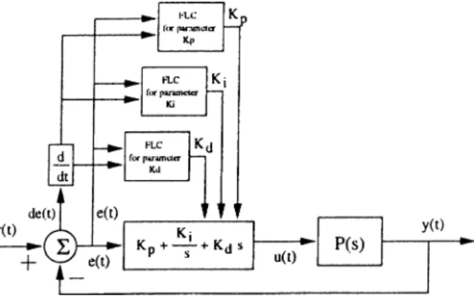
The system structure under consideration is given in Fig.4.1. Here P(s) is the transfer function of the plant and the FLCs are the fuzzy logic systems tuning each parameter of the PID controller. The objective is to construct a rule base and to set the related membership functions for each FLC to get a satisfactory output response.
Figure 4.1; System structure under investigation
4.1.1
Rule-Base Construction
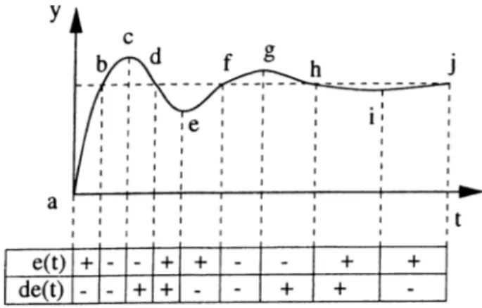
The fuzzy rules for the PID controller is derived from the examination of a typical step response given in Fig.4.2. In this figure the sign of error(e(t)) and increment of the error(de(t)) are given in a tabular form. The points where e(t) and de(t) changes their signs are labeled on the step response with the letters a, b, c, j. The following argument for the derivation of the rules will be similar to the work done by Tomizuka et.al.(1993)[4].
Consider the point a given on the step response in Fig.4.2. At the beginning a big control signal is required in order to achieve a fast rise time. To produce a big control signal, the PID controller should have a large proportional gain,
a large integral gain and a small derivative gain. From point a to b the error is positive and big. The increment of error is negative and the magnitude seems to be big in the middle of these points. For some slow responding systems at
I
points closer to a, the magnitude of the increment of the error can be small. From the above discussion one may derive the following rules:
if “e(t) is PB” and “de(t) is NB” then "A'p is BIG” , if “e(t) is PB” and “de(t) is NB” then "A', is BIG” , if “e(t) is PB” and “de(t) is NB” then “ A'^ is SMALL” .
(4.1)
if “e(t) is PB” and “de(t) is NS” then ‘"A'p is BIG” , if “e(t) is PB” and “de(t) is .NS” then “ A', is BIG” , if “e(t) is PB” and “de(t) is NS” then “ A'^ is SMALL” .
(4.2)
Figure 4.2: A typical step response of a system.
Here PB, NS stands for Positive Big and Negative Small which are fuzzy sets. As it is clear the first letter stands for the sign and the second for the magnitude. Fuzzy sets defined on the domain of error and increment of the error are labeled with the following: NB, NM, NS, ZE, PS, PM, PB. Here M stands for Medium, ZE for zero.
At points closer to b the error is close to zero but the increment of the error is negative and big. At this point to avoid a large overshoot the PID
controller should have a small proportional gain, a large derivative gain, and a small integral gain. Thus the following rules are given:
if "e(t) is ZE” and '‘de(t) is NB"’ then “ Ap is SMALL” , if '‘e(t) is ZE” and “de(t) is NB” then “ A',· is SM.ALL” , if "e(t) is ZE” and “de(t) is NB” then “ A j is BIG” .
(
4
.3
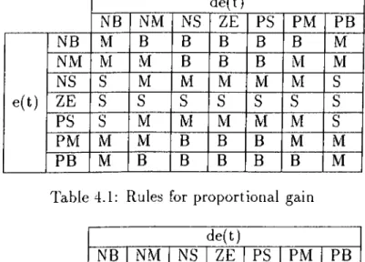
)By using similar arguments, a set of rules, as shown in Tab.4.1, may be used to adapt the proportional gain. The tuning rules for derivative gain and integral gain are given in Tab.4.2 and Tab.4.3. respectively.
de(t) NB NM NS ZE PS PM PB e(t) NB M B B B B B M NM .M M B B B .M M NS
s
M M M M Ms
ZEs
s
s
s
s
s
s
PSs
M M M M Ms
PM M M B B B M M PB M B B B B B MTable 4.1: Rules for proportional gain
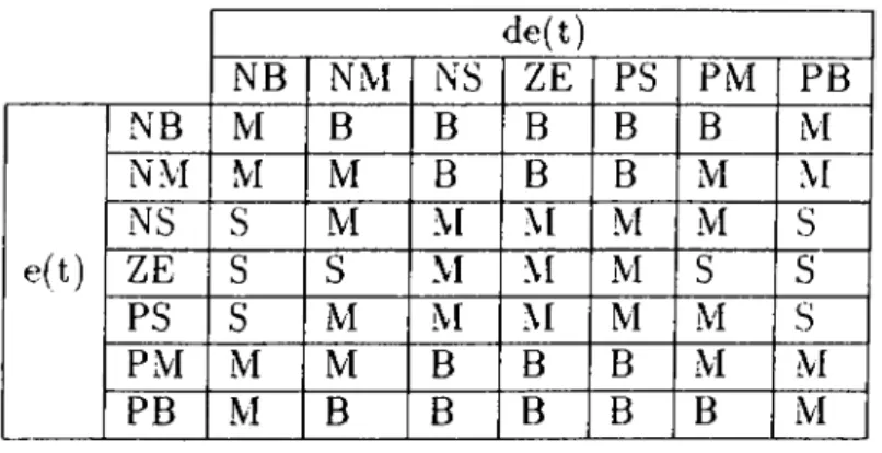
Table 4.2: Rules for derivative gain de(t) NB NM NS ZE PS PM PB e(t) NB M
s
s
s
s
s
M NM M Ms
s
s
M M NS B M M M M M B ZE B B M M M B B PS B M M M M M B PM M Ms
s
s
M M PB Ms
s
s
s
s
MIn these tables, “S” , “ M” , and “ B” refer to “Small” , “ Medium” , and “Big” , respectively.
e(t) NB I m NS ZE PS PM PB NB M M M M NM B M M M M B NS B B M M M B B de(t) 'ZE B B M M M B B PS B B M M M B B PM B M M M M B PB M M M M Table 4.3: Rules for integral gain
4.1.2
FLC Structure
The membership functions for the linguistic variables error and increment of error are given in Fig.4.3. All the membership functions of error and its in crement are defined on the interval [0,1]· The actual domain of the linguistic variable error is the unit interval but the domain of its increment depends on the simulation step size and its variation is much smaller than the unit interval. Therefore a normalization procedure is applied to the increment of the error before the fuzzification operation. The scaling factor in this normalization op eration is chosen so that the increment of error is large enough to span the interval [-1, 1].
In designing the controller individual rule-based inference is chosen. There fore the fuzzification operation is performed as explained in the example of Sec.3.3.1. The fuzzy set operations used in the design are the same as given in Def.3. Mamdani implication is used in firing each rule.
Figure 4.3: Membership functions for error and increment of error
After firing each rule in the rule-base of a parameter there will be clipped version of the fuzzy sets given in Fig.4.4 for the linguistic variables Kp, Ki,
and Kd- The gains of the PID controller are always positive. Therefore before the scaling of the domain of these membership functions they must be shifted to a reasonable amount.
Figure 4.4: Membership function for the variables /Fp, A'i, and Kd
In general the determination of this shift and the scaling is a trial and error procedure. Based on extensive simulation study on various processes, a rule of thumb for determining the range of Kp and the range of Kd is given as
^^PyTTlin 0.*32A(;7., Kp^jTidx
Kd,min = OMKcrPcr, Kd,max = 0.15A'cr ^cr·
where Kcr and Per are the gain and the period of oscillation at the stability limit under P-control[12]. Tomizukaet.al.[4] uses this method to set the domain of the membership functions for the gains because in their work they related the integral gain to the proportional and derivative gain with a constant a. In our design all PID gains are considered to be independent of the each other and each of them have a separate rule base. In the simulations the ranges of the membership functions are found by first applying this method and then making a fine tuning.
4.1.3
Simulations and Results
The fuzzy parameter tuning has been tested on a variety of processes. One of them is given here. The plant transfer function is given in Eqn.4.4. Ziegler- Nichols PID tuning results in the following gains for this plant.
P .( 5 ) = _____________
1
_____________5
·^ +63
^ +11
.^: +6
’ (4.4) Ap = 36.0000, K, = 38.0047. A'j = 8.5253.The membership functions for error and change of error is the same as given in Fig.4.3. The normalization constant for the increment of the error was chosen to be 20.
The membership functions for A'p, A',, and Kd are given in Fig.4.5. These figures show the effective membership functions taking into account the shift and scaling operations in the denormalization stage.
Computation o f the parameters Ap, A',, and
Kd
Assume that the error and its increment is e* and de*, respectively. Let us take one of the entries of Tab.4.1.
if “e(t) is PS” and “de(t) is NS” then ~Kp is MEDIUM” . (4.5)
First the fuzzification operation must be applied to the crisp values e* and de*. Since individual-rule based inference is chosen in the calculations, the fuzzification operation will result the following two value, fj,ps{e*) and /i^5(de*).
The set operations were chosen as the min, max, and standard complement. So the truth value of this rule will be calculated as :
Hi = min(/ips(e*),/iw^s(de*)). (4.6)
For the implication operation, Mamdani implication is chosen. Therefore the implied fuzzy set for the proportional gain is calculated as,
Figure 4.5: Membership function for the variables Kp, Ki, and
= min{ (4.7)
This procedure is performed to all of the rules in the rule table and all of these clipped fuzzy sets are combined with the union operator, max(·).
fi{u) = max(^jv/(u)^//M (w)^,---,/^M (w)^). (4.8)
This way the final fuzzy set for the parameter is obtained. This value must be converted to a crisp value by the defuzzification operation. In this thesis the center of gravity is used as the defuzzification operation. Applying this to the fuzzy set gives the value for the proportional gain.
r . . ^ E!=1
(4.9)
This operation is repeated for A", and Kj, in the same way. The output of the system with Ziegler-Nichols PID controller and the output of the system where the parameters are tuned with FLCs are compared in Fig.4.6. The PID parameters calculated by the FLCs are given in Fig.4.7
The designed controller is tested for a plant ^
2
(5
) given below, which may be considered as a slightly perturbed version of the plant given by Eqn.4.4.Figure 4.6: Comparison of the step responses.
So4id:Kp, OaaittfdiKl, Oo«ecl;Kd
Figure 4.7: PID parameters determined by the FLCs.
P
2
W =^3
^ 4_j24
. g (4.10)The output waveforms for the fuzzy PID and the classical PID are compared in Fig.4.8. The PID parameter variations are given in Fig.4.9.
The proposed gain scheduling scheme uses fuzzy rules and reasoning to determine the PID parameters. This fuzzy PID controller design has been tested on various processes in simulation, and satisfactory results are obtained. From Fig.4.9 it is seen that with the proposed PID controller the overall system is at least as insensitive to the parameter variations as the system with PID controller, having fixed gains.
Figure 4.8; Comparison of the step responses.
Solid; Kp. Oashed;Ki, Dotted: Kd
Figure 4.9: PID parameters determined by the FLCs.
4.2
Lead-Lag Controller Design
For this design problem the structure of the overall system is as shown in F'ig.4.10. In this figure P(s) is the plant transfer function. There are two parameters in the lead-lag controller to be determined, namely a and T.
As in the case of PID controller we need two FLC blocks, one for a and one for T. The effect of the variations of the parameters a and T on the output of the system seems to be in the same direction. Therefore the parameter T is fixed and only a is tuned with FLC. The value of T is determined with a classical design method.
r(t)
+
Figure 4.10: System structure under investigation
4.2.1
Rule-Base Construction
To determine the effect o f the parameters on the step response of the system, many simulation have been performed. In all of the cases the effect of a and T turn out to be the same. Therefore only the parameter a will be investigated. The reason to choose the parameter a for the tuning is that, for values of a less than 1 the controller is a phase lag controller and for a greater than 1 it is a phase lead controller. The value of T is set to 1.
In Fig.4.11 and Fig.4.12 the variations of the step responses of two different plants, given above with respect to the parameter a are shown. In these figures the solid lines are the output of the plants Pi(s) and P2{s) without a controller.
These plants have the following transfer functions:
= / ’=(») = t oS t s:·
Figure 4.11: Step responses of Pi{s) for a=0.01, 0.3, 0.7, 1, 2, 5, 10.
Figure 4.12: Step responses of /
2
(3
) for a=0.01, 0.3, 0.7, 1, 2, 3, 4.In Fig.4.11.(a) the step responses for a = 1, 2, 5, 10 are given. As the value of a increases the rise time decreases and the overshoot increases. In Fig.4.11.(b) the step responses for a = 0.01, 0.5, 0.7, 1 are shown. Here the
same behavior is observed. The overshoot of the step response is proportional to the parameter a whereas there is an inverse relationship between the rise time ot the system and the parameter a. In F'ig.4.T2.(b) the step responses for a = 1, 2, 3, 4 are given. As the value of a increases the rise time decreases and the overshoot increases. In Fig.4.12.(b) the step responses for a = 0.01, 0.5, 0.7, 1 are shown. Here a different behavior is observed. In this case both the overshoot of the step response and the rise time of the system are inversely proportional to the parameter a.
For the output of a system it is desired to have a short rise time and no overshoot and oscillations. To have a short rise time we have to chose a large value for a, say örnax· But for large a we get a large overshoot and rather an oscillatory response at the output. One possible way is to set the value of a to a large value in the beginning and reduce it when the system output is about to catch the reference signal. From Fig.4.2 at the beginning the error will be a member of the fuzzy set PB and its increment will be a member of the fuzzy set NB (or NS). So using these arguments one may state the following rules:
if ^^e(t) is PB” and ‘‘de(t) is NB” then “a is LA7” , if "e(t) is PB” and ‘^de(t) is NS” then ‘‘a is LA7” , if "e(t) is ZE” and ^^de(t) is NB” then "a is LA6” .
(4.11)
The meaning of the linguistic values LA7, LA6, and the rest are given in F’ig.4.13. Using this discussion on the effect of the variation of a to the output a rule-base is constructed as given in Tab.4.4.
Figure 4.13: Membership functions of the linguistic variable a
The membership functions for the parameter a are chosen so that they all
e(t) NB NM NS ZE PS PM PB NB LA3 LA4 LA4 LAo T a^ LA7 LA7 NM LA3 LA3 LA4 LA4 LAo LA6 LA7 NS LA2 T X 3 LA3 LA4 LA4 LA5 LA6 de(t) ~ZET~ LA2 LA2 LA3 LA3 LA4 LA4 LAo PS LAI LA2 LA2 LA3 LA3 LA4 LA4 PM LAI LAI LA2 LA2 LA3 LA3 LA4 PB LAI LAI LAI LA2 LA2 LA3 LA3 Table 4.4: Rules for lead-lag parameter a
equally share the domain in the intervals [0,1] and [1 a,,
4.2.2
FLC Structure
In Fig.4.13 the value of ttmax is chosen to be a large number to have a short rise time. The membership functions for the error and its increments are as in the case of PID controller design. Again a normalization factor is used before the fuzzification operation such that the increment of error spans the interval [-1.1]·
Individual rule-based inference is used to fire all the rules in the rule-base. Therefore the fuzzification operation is the same as in the previous section. The fuzzy set operations used in the design are the same as given in Def.3. As in the previous design here also Mamdani implication is used as the inference engine. Since the membership functions for the parameter a are defined on its actual domain there is no need for a denormalization stage.
4.2.3
Simulations and Results
This fuzzy parameter tuning scheme for the lead-lag type controller is applied to various systems. Simulations showed that a variety of processes can be satisfactorily controlled by the fuzzy parameter tuned lead-lag controller. One o f the simulations is performed with a plant whose transfer function is given
in Eqn.4.12 . A phase-lead controller based on a classical design for this plant results in a controller whose transfer function is given in Eqn.4.13
^3(^) = 2.500 (4.12)
s{s -I- 25) ’
0.016s 4- 1
0
.002
s +1
■ (4.13)C(s) =
In this design the parameter a and T are
8
and 0.002 respectively[L3]. In the proposed fuzzy parameter tuning algorithm the value of T is not changed. It is set to a value obtained in a classical design. Therefore for this plant the value of T is set to 0.002.Figure 4.14: Comparison of the step responses of ^
3
(3
) with the two different controller.The normalization constant for the increment of error is chosen to be 9. The membership function for the error and its increment is as mentioned in Sec.4.
2
.2
. The membership functions for the linguistic values of a are taken as given in Fig.4.13. For this simulation amax is set to 100. Again Mamdani Implication is used in interpreting the meaning of the rules.The step responses of the system Pz{^) with the two different controllers given above, one classical and one fuzzy, are given in Fig.4.14.(a). In
Fig.4.14.(b) the variation of the parameter a is given. From the figure it is seen that at the beginning a takes large values and as the output approaches ,the desired reference signal the FLC reduces the parameter a. This FXC has been tested on various systems which may be considered to be the plant P^is) with distorted coefficients. One of these plants is given below:
P.fsi - _
5 0 0 0_
s2+24a+l·
The step responses corresponding to the fuzzy tuned lead-lag controller and the classical design is given in Fig.4.15.(a)
Figure 4.15: (a) Step responses of P