RESILIENT PI AND PD CONTROLLER DESIGNS
FOR A CLASS OF UNSTABLE PLANTS WITH I/O DELAYS* H. ¨OZBAY †, A. N. G ¨UNDES¸ ‡, §
Abstract. In [8] we obtained stabilizing PID controllers for a class of MIMO unstable plants with time delays in the input and output channels (I/O delays). Using this approach, for plants with one unstable pole, we investigate resilient PI and PD controllers. Specifically, for PD controllers, optimal derivative action gain is determined to maximize the allowable controller gain interval. For PI controllers, optimal proportional gain is determined to maximize a lower bound of the largest allowable integral action gain.
Key words:PID Control, Time Delay, Unstable Systems
1. Introduction
PID controllers are still very popular in many control applications thanks to their simple structure, [1, 5]. Design of PID controllers for delay systems is still an active research area, see for example the recent book [15], and its references. In this paper we consider unstable plants with time delays. It is clear that, even for delay-free systems, not all unstable plants are stabilizable by a PID controller (strong stabilizability is a necessary condition for stabilization by a PID controller, and there are bounds on the order of strongly stabilizing controllers, [8, 17, 19]). Moreover, right half plane poles and zeros in the plant transfer matrix, as well as time delays in the input and/or output channels (I/O delays) of the plant, impose additional restrictions on the feedback controllers, see e.g. [6, 7, 11, 18, 21].
Recently, PID controllers are designed in [20] under specified gain margin and sensitivity constraints, and in [14] under an H∞ performance condition. PID controller tuning rules are
also discussed in [9, 16] under different optimality conditions. For SISO unstable systems with delays PID controller tuning has been studied in [10, 13]. An extension of predictive control is used in [3] to derive PID controllers for a class of MIMO unstable plants with delays.
In a recent work [8] obtained PID controllers from a small gain argument for a class of MIMO unstable plants with delays in the input and output channels (I/O delays). In this paper we use the results of [8] for plants with one unstable pole, and investigate stabilizing PI and PD controllers with the largest allowable interval for the controller gain. This is an important problem to study, because sensitivity of the closed loop stability to perturbations in the controller coefficients can be minimized this way, and hence resilient PI and PD controllers (see e.g. [15] and its references for a discussion of this issue) can be obtained. There are many important practical examples of plants with single unstable pole and time delays, see e.g. [2, 10, 13, 15, 18] and their references.
Remaining parts of the paper are organized as follows. Preliminary results from [8] are summarized in Section 2. Main results on PD controller design are given in Section 3, and the results on PI controller are given in Section 4; concluding remarks are made in Section 5.
* This work was supported in part by the European Commission under contract no. MIRG-CT-2004-006666 and by T ¨UB˙ITAK BAYG and EEEAG under grant no. EEEAG-105E065 and EEEAG-105E156.
†Dept. Electrical & Electronics Eng., Bilkent Univ., Ankara, 06800 Turkey, [email protected]
Dept. Electrical & Computer Eng., Univ. of California, Davis, CA 95616, U.S.A., [email protected]
§Manuscript received May 22, 2007.
2. Problem Definition and Preliminary Results
Consider the linear time invariant (LTI) feedback system shown in Figure 1, where C is the controller to be designed and GΛ := ΛoGΛi is the plant with r inputs and r outputs. Here G is the delay free part of the system which is assumed to be finite dimensional. Time delays
in the input and output channels of the plant are represented by their transfer matrices as Λ• = diag £e−sh•
1, . . . , e−sh•r¤, where, h•
j is the jth channel input (when • = i) or output (when • = o) delay, for 1 ≤ j ≤ r. - h - C - h? - ΛoGΛi -6 − yref e v u y
Figure 1. Feedback system Sys(GΛ, C) with GΛ= ΛoGΛi. Transfer matrix Hcl from (yref, v) to (u, y) is
Hcl = · C(I + GΛC)−1 −C(I + GΛC)−1GΛ GΛC(I + GΛC)−1 (I + GΛC)−1GΛ ¸ . (1)
We consider the proper form of PID controllers, [5],
C(s) = Cpid(s) = Kp+Ksi + τKd s ds + 1
, (2)
where Kp, Ki, Kd are real matrices and τd > 0. But we will restrict ourselves to PI and PD
controllers, i.e., Cpi= Kp+Ksi and Cpd= Kp+ τKds+1d s respectively.
Definition. The feedback system Sys(GΛ, C) is stable if all entries of Hcl are in H∞. We define Spid, Spi, Spd to be the sets of all PID, PI and PD (respectively) controllers stabilizing the
feedback system Sys(GΛ, C).
Assumptions.
(A1) G admits a coprime factorization in the form G(s) = Y (s)−1X(s) = X(s)Y (s)−1 where X ∈ Hr×r
∞ , and Y (s) = (as+1)(s−p) I. Here p ≥ 0 is the unstable pole of the plant, and a > 0 is arbitrary.
(A2) X(0) = (s − p)G(s)|s=0 is nonsingular.
Proposition 2.1. [8] Consider the plant GΛ = ΛoGΛi, where G satisfies (A1) and (A2). i) PD-design: Choose any ˆKd∈ Rr×r, and τd> 0. Define ˆCpd:= X(0)−1+τKdˆs+1ds and
ΦΛ:= s−1((s − p)GΛ(s)ˆcpd(s) − I)
e
ΦΛ:= s−1(bcpd(s)(s − p)GΛ(s) − I).
If 0 ≤ p < max{kΦΛk−1∞, keΦΛk−1∞}, then for any α > 0 satisfying
0 < α < max{kΦΛk−1∞ − p , keΦΛk−1∞ − p } , (3) the controller ˆCpd(s) = (α + p) ˆCpd(s) is in Spd.
ii) PID-design : Let Cpd be as above, and define Hpd := GΛ(I+CpdGΛ)−1, Υ := Hpd(s)Hpd(0) −1−I
s ,
e
Υ := Hpd(0)−1Hpd(s)−I
s . Then, for any γ ∈ R satisfying
0 < γ < max{kΥk−1∞ , k eΥk−1∞}, (4)
the PID-controller given in (5) is in Spid,
Cpid(s) = Cpd(s) +γαX(0) −1
If (3) and (4) are satisfied for ˆKd= 0 then (5) with ˆKd= 0 is a PI controller in Spi. ΛG(s) = · 1 0 0 180 (s+6)(s+30) ¸
This result appears in [8] for systems with possibly uncertain time delays, but for our purposes fixed time delays version stated above is sufficient. Now consider the plants with input delays only satisfying the following structural assumption.
Assumption (A3). GΛ(s) = G(s)Λi(s), with G(s) = 1
s−pG0ΛG(s) where G0 is a
non-singular constant matrix and ΛG(s) is a stable diagonal matrix with ΛG(0) = I, i.e., ΛG(s) =
diag[g1(s), . . . , gr(s)], where g1(s), . . . , gr(s) are stable proper transfer functions with gj(0) = 1,
for all j = 1, . . . , r. Note that with A3 we have X(0) = G0 and earlier assumptions A1 and A2 are satisfied. Moreover, this assumption results in a diagonal structure in the input sensitivity matrix, as demonstrated below. An example for A3 is the transfer matrix of a distillation column with input channel delays, [4], GΛ(s) = 1
s G0 ΛG(s)Λi(s), where G 0 = · 3.04 − 278.2/180 0.052 206.6/180 ¸ , ΛG(s) = · 1 0 0 180 (s+6)(s+30) ¸ .
2.1. PD Control of Systems With Input Delays. Let A3 hold, and define ˆKd= ˜KdiX(0)−1=
˜
Ki
dG−10 . Then, the PD controller of Proposition 2.1 can be re-written as Cpd(s) = (α +
p) ³ I + ˜Ki dτds+1s ´ G−10 . Then choosing ˜Ki
d := diag[q1i, . . . , qri], we have a diagonal input
sen-sitivity matrix Si(s) = (I + Li(s))−1, where Li(s) = (α + p)(s − p) µ I + ˜Kdi s τds + 1 ¶ ΛG(s)Λi(s).
Proposition 2.1 gives a lower bound on the largest controller gain interval: p < (α + p) <
k ˜ΦΛk−1∞. For the purpose of designing a resilient controller, we would like to maximize the size
of this interval. That is equivalent to minimizing
µi := k ˜ΦΛk∞= k ΛF i(s) − I s + ˜K i d ΛF i(s) τds + 1k∞ (6)
where ΛF i:= ΛGΛi. Therefore, in Section 3 we will study the problem of minimizing µi defined
by (7) over the free parameters q1i, . . . , qir, where fji(s) := gj(s)e−h
i js µi = max j k fi j(s) − 1 s + q i j fi j(s) τds + 1k∞. (7)
We should point out that with the dual structural assumption GΛ(s) = Λo(s)G(s), with G(s) = 1
s−pΛG(s)G0 where G0 and ΛG(s) are as in A3, a similar problem can be defined for the
output delay case, where kΦΛk∞ is minimized. The case where both input and output delays
exist is more difficult, but if either output or input delays are equalized in all the channels, then that would lead to the same problem of minimizing either kΦΛk∞ or k ˜ΦΛk∞, see [12].
2.2. PI Control of Systems With Input or Output Delays. Now consider PI controllers with the proportional part Cp = (α + p)X(0)−1, where α satisfies (3). The PI controller is then
in the form
Cpi(s) = (α + p)X(0)−1+γαs X(0)−1 (8)
where γ satisfies (4). Recall that, under the structural assumption A3, we have X(0) = G0. An interesting problem in this case is to find the largest allowable interval for γ, for a fixed α satisfying (3).
Note that in this case Hpd(s) = Hp(s) = GΛ(I + CpGΛ)−1 = (I + GΛCp)−1GΛ. As in the above discussion on PD controller design we will assume that A3 holds and α is in the interval
0 < α < k ˜ΦΛk−1∞ − p. In this case, since the derivative term is absent, we have ˜ΦΛ = Λ(s)−Is , where Λ = ΛGΛi. Then a lower bound for the maximum interval for the allowable “integral
action gain” γ is found from (4) where eΥ = αΛ(s)((s−p)I+(α+p)Λ(s))s −1−I. It is easy to see that in the dual case, where output delays are considered, and the added restriction 0 < α < kΦΛk−1∞−p,
we have Υ = αΛ(s)((s−p)I+(α+p)Λ(s))s −1−I, where Λ = ΛoΛG. Thus, it is interesting to study the
upper bound γmax for γ where
γmax:= k α s−pΛ(s)(I + α+ps−pΛ(s))−1− I s k −1 ∞ (9) as a function of α satisfying 0 < α < kΛ(s) − I s k −1 ∞ − p (10)
where Λ(s) = ΛG(s)Λi(s) for the input delay case and Λ(s) = Λo(s)ΛG(s) for the output delay
case.
3. Optimal Derivative Action Gain
Recall from (7) that we are interested in solving the following problem: given h > 0 and a stable transfer function g(s) with g(0) = 1, let f (s) = g(s)e−hs, and find q ∈ R such that µ is minimized, where
µ = kf (s) − 1
s + q
f (s)
τds + 1k∞ , τd→ 0. (11)
We shall denote the optimal solution by qopt. This is a single parameter scalar function H
∞
norm minimization problem and it can be solved numerically using brute force search. More precisely, such an algorithm would perform the following steps:
0. Choose the candidate values of q = q1, . . . , qN, over which the optimization is to be done,
and the frequency values ω = ω1, . . . , ωM over which the norm (cost function) is to be
computed.
1. For k = 1, . . . , N and ` = 1, . . . , M compute Ψ(qk, ω`) := |f (jωjω``)−1+ qk jτf (jωdω`+1`) | .
2. Define µ(qk) := max`Ψ(qk, ω`).
3. Optimal q is qopt = arg min
kµ(qk).
As an example, consider the distillation column transfer matrix given in Section 2, where g1(s) = 1 and g2(s) = (s+6)(s+30)180 . Optimal derivative gains are computed in [8] (see Figure 4 of [8]) using the numerical procedure given above. However, this procedure is sensitive to the number of grid points chosen for q and ω. So, it would be useful if one could derive a closed form expression for the solution, at least for the simplest case g(s) = 1, i.e. f (s) = e−hs. It turns out that this is possible, and we claim that qopt(h) = sin(2.33)
2.33 h = 0.31 h for f (s) = e−hs. In the rest of this section we discuss how qopt can be computed directly for a class of functions f .
Note that (11) is a min-max problem
µ = min
q∈R maxω∈R Ψ(q, ω) (12)
where Ψ(q, ω) = |f (jω)−1jω + q jτf (jω)
dω+1| , τd→ 0. Let us now consider the max-min problem where minimization over q is done for each fixed ω. In this case, it is easy to show that optimal q is
where ρ(ω) = |f (jω)| is the magnitude and φ(ω) = ∠f (jω) is the phase of f (jω). Inserting (13) into Ψ(q, ω) we obtain Ψ(qopt(ω), ω) = ¯ ¯ ¯ ¯ρ(ω) − cos(φ(ω))ω ¯ ¯ ¯ ¯ =: η(ω). (14)
Therefore, solution of the max-min problem is
qo = − 1
ωo
sin(φ(ωo))
ρ(ωo)
(15) where ωo is maximizing η(ω). It is very easy to find qo, we only need to search for ωo. Whereas
the min-max problem requires two dimensional search.
Example. Consider f (s) = e−hs, h > 0. Then ρ(ω) = 1 and φ(ω) = −hω. Hence η(ω) =
|1−cos(hω))ω |. It is easy to show that the ω value maximizing this function is the solution of
cos(hω) + (hω) sin(hω) = 1. That gives hωo = 2.33 rad., qo= 0.31 h, and it matches qopt(h).
Now it remains to be shown that qo given in (15) is equal to the solution qopt of the original
problem defined by (12), at least for a large class of functions f (s), including the above example. For this purpose, we need to show that the pair (ωo, qo) is a saddle point for the min-max problem
(12), i.e. the following inequalities hold
Ψ(qo, ω) ≤ Ψ(qo, ωo) ≤ Ψ(q, ωo) ∀ q, ω ∈ R . (16)
First note that by the definition of qopt(ω) we have Ψ(qopt(ω), ω) ≤ Ψ(q, ω) for all q ∈ R and
ω ∈ R. In particular, setting ω = ωo in this inequality we obtain the second part of (16), namely
Ψ(qo, ωo) ≤ Ψ(q, ωo) ∀ q ∈ R . (17)
For the first inequality of (16), when τd= 0, we have Ψ(qo, ω) = |Ψ(qopt(ω), ω)+∆q(ω) f (jω)|,
where ∆q(ω) = qo− qopt(ω). We claim that
|Ψ(qo, ω)|2 = |η(ω)|2+ |∆q(ω)|2|ρ(ω)|2 ∀ ω. (18)
To see this let us define the real and imaginary parts R(ω) + jI(ω) := f (jω)−1jω + qopt(ω) f (jω). Similarly, let Rf(ω) + jIf(ω) := f (jω) be the real and imaginary parts of f . With these definitions we have RfR + IfI = 0, which implies (18).
Assumption A4. The function f (s) is such that Γ(ω) := η2
o− η2(ω) − |∆q(ω)|2ρ2(ω) ≥ 0 ∀ ω
where η(ω) is defined by (14), ηo = maxωη(ω), and equations (13) and (15) define ∆q(ω) =
qo− qopt(ω).
Now with A4, (18) and ηo = Ψ(qo, ωo), we have Ψ(qo, ω) ≤ Ψ(qo, ωo) ∀ ω ∈ R which is the
first part of (16). In summary, we have proven the following result.
Proposition 3.1. Let f (s) = g(s)e−hs, with g ∈ H∞, g(0) = 1 and h > 0, satisfy A4. Then, qopt = q
o where
qopt = arg min
q∈Rk f (s) − 1 s + q f (s) τds + 1 k∞ , τd→ 0 qo = −ω1 o sin(φ(ωo)) ρ(ωo) , where ωo is maximizing η(ω) := |ρ(ω)−cos(φ(ω))ω |.
Example. Consider the first channel in the distillation column example, where f (s) = e−hs, h > 0. Figure 2 shows Γ/h versus ω. Since Γ(ω) ≥ 0 for all ω, A4 is satisfied, hence the
formula qopt = 0.31 h is valid. Now for the second channel in the distillation column example,
f (s) = 180
(s+6)(s+30)e−hs, Figure 3 illustrates that A4 is satisfied. Figure 4 shows qopt and µ versus
10−1 100 101 102 103 −0.1 0 0.1 0.2 0.3 0.4 0.5 0.6 ω Γ(ω)/h versus ω for h=0.2, 0.6, 1.0 h=0.2 h=0.6 h=1.0
Figure 2. Γ(ω)/h versus ω for f (s) = e−hs.
10−1 100 101 102 103 −0.1 0 0.1 0.2 0.3 0.4 0.5 0.6 0.7 Γ(ω)/h versus ω for h=0.2, 0.6, 1.0 h=1.0 h=0.6 h=0.2
Figure 3. Γ(ω)/h versus ω for f (s) = e−hs180 (s+6)(s+30). 0 0.2 0.4 0.6 0.8 1 0 0.1 0.2 0.3 0.4 0.5
µ versus h and qopt versus h
h µ/2 q
opt
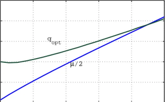
Figure 4. qopt and µ versus h.
interval for the control gain shrinks with increasing h. Note that qopt in Figure 4 is in perfect agreement with Figure 4 of [8].
An interesting problem arising in this context is to characterize the class of functions f (s) =
g(s)e−hs, g ∈ H
∞, g(0) = 1, h > 0, satisfying A4. At the moment we do not have a definite
answer to this question. As shown for the distillation column example, A4 holds for many interesting classes of f . In particular, it holds for all f in the form f (s) = 1+τ se−hs, and f (s) =
e−hs 1−τ s1+τ s, for all τ ≥ 0 and h > 0. But, there are also many important functions for which it does not hold. For example, f (s) = e−s 1−s
when τ ≤ 0.2. Similarly, A4 holds for f (s) = e−s 1+s
1+τ s when τ ≤ 1.02, but it is violated when
τ ≥ 1.05.
4. Integral Action Gain in PI Controller
We now study the bound γmax on the integral action gain γ defined by (9), where Λ(s) is a given diagonal matrix in the form diag[f1(s), . . . , fr(s)] with fk(s) = gk(s)e−hks, gk ∈ H∞, gk(0) = 1, hk > 0, and α satisfies (10) which is equivalent to p < α + p < minkkfk(s)−1
s k−1∞. Clearly, γmax−1 = max k k α s−pfk(s)(1 + α+ps−pfk(s))−1− 1 s k∞. (19) Let us define θ := max k θk where θk := k fk(s) − 1 s k∞ . (20)
Then, a necessary condition for the results stated in Proposition 2.1 is 0 < αθ < 1 − pθ. After a simple algebra, it can be shown that (19) implies
γ? := α 1 − (α + p) θ1 + p θ ≤ γmax . (21) The lower bound γ?, found in (21) for γmax, is between 0 and α, and it decreases with increasing
θ. Note that θ−1 is also an upper bound for the proportional gain (α + p). Therefore, the level of
difficulty in controlling the system increases with increasing θ. The other difficulty comes from the C+ pole of the plant: as p increases γ? decreases.
Example. Let fk(s) = e−hks. Then, θk = hk, and θ is the largest time delay in the system.
Now consider f1(s) = e−h1s, and f2(s) = (s+6)(s+30)180 e−h2s. In this case we have θ1 = h1, and
θ2 = 0.2 + h2. Since the norm in (20) is attained at ω = 0 for both f1 and f2 and the phase of
f2(jω) near ω ≈ 0 is −0.2 ω, we can see θ2 as the “effective time delay” in the second channel. Then, θ = max{h1, 0.2 + h2} is the largest effective time delay.
In the light of (21) an interesting problem to study is to find the optimal α maximizing γ?,
subject to 0 < αθ < 1 − pθ. It is easy to see that in this sense the optimal α is
α? = 1 − pθ2θ (22)
and the corresponding maximal γ? is
γ?,max= α2? (1 − pθ)(1 + pθ). (23)
Equations (22) and (23) show once again that the difficulty level increases with increasing pθ, where p is the right half plane pole and θ can be seen as the maximal “effective time delay” in the system.
5. Conclusions
PI and PD controller design problems are studied for unstable systems with delays in the input/output channels. The results of [8] are used for plants with single right half plane pole. For PD controller design, optimal derivative action gain is determined for maximizing the interval for the overall controller gain. For PI controller design, optimal proportional gain is calculated for maximizing the interval for the integral action gain. With these results resilient PI and PD controllers can be designed for the class of plants considered. Examples illustrated difficulty of controller design for plants whose products of unstable pole with effective time delay are large. Acknowledgement: The authors would like to thank Prof. A. B. ¨Ozg¨uler for fruitful discus-sions.
References
[1] Astr¨om, K. J., and Hagglund, T. PID Controllers: Theory, Design, and Tuning, Second Edition, Research Triangle Park, NC: Instrument Society of America, 1995.
[2] Enns, D., H. ¨Ozbay and Tannenbaum,A. “Abstract model and controller design for an unstable aircraft,” AIAA Journal of Guidance Control and Dynamics, March-April 1992, vol. 15, No. 2, pp. 498–508.
[3] Fliess, M., Marquez, R. and Mounier,H. “An extension of predictive control, PID regulators and Smith predictors to some linear delay systems,” Int. J. Control, vol. 75 (2002), pp. 728–743. [4] Friedland, B., Control System Design, An Introduction to State Space Methods, McGraw-Hill, 1986. [5] Goodwin, G. C., Graebe,S. F. and Salgado,M. E. Control System Design, Prentice Hall, 2001. [6] Gu, K., Kharitonov,V. L. and Chen,J. Stability of Time-Delay Systems, Birkh¨auser, Boston, 2003. [7] G¨um¨u¸ssoy, S., ¨Ozbay, H.“Remarks on strong stabilization and stable H∞ controller design,” IEEE
Transactions on Automatic Control, vol. 50, (2005), pp. 2083–2087.
[8] G¨unde¸s, A. N., ¨Ozbay,H. and ¨Ozg¨uler,A. B. “PID controller synthesis for a class of unstable MIMO plants with I/O delays”, Automatica, vol. 43, No. 1, January 2007, pp. 135–142.
[9] Kristiansson, B., Lennartson, B.“Robust and optimal tuning of PI and PID controllers,” IEE
Pro-ceedings - Control Theory Appl. vol. 149 (2002), pp. 17–25.
[10] Lee, Y., Lee, J. and Park, S. “PID controller tuning for integrating and unstable processes with time delay,” Chemical Engineering Science, vol. 55 (2000), pp. 3481–3493.
[11] Niculescu, S.-I., Delay Effects on Stability: A Robust Control Approach, Springer-Verlag: Heidelberg, LNCIS, vol. 269, 2001.
[12] ¨Ozbay, H., and G¨unde¸s,A. N. “Resilient PI and PD Controllers for a Class of Unstable MIMO Plants with I/O Delays”, Proc. of the 6th IFAC Workshop on Time Delay Systems, L’Aquila, Italy, July 2006
[13] Poulin, E., Pomerleau, A. “PI Settings for Integrating Processes Based on Ultimate Cycle Informa-tion,” IEEE Trans. on Control Systems Technology, vol. 7 (1999), pp. 509–511.
[14] Saeki, M., “Fixed structure PID controller design for standard H∞ control problem,” Automatica,
vol. 42 (2006), pp. 93–100.
[15] Silva, G. J., Datta, A. Bhattacharyya, S. P.PID Controllers for Time-Delay Systems, Birkh¨auser, Boston, 2005
[16] Skogestad, S., “Simple analytic rules for model reduction and PID controller tuning,” J. of Process
Control, vol. 13 (2003), pp. 291–309.
[17] Smith, M. C., Sondergeld, K. P. “On the order of stable compensators,” Automatica, vol. 22 (1986), pp. 127–129.
[18] Stein, G., “Respect the Unstable,” Bode Lecture IEEE CDC Tampa, FL, December 1989, see also
IEEE Control Systems Magazine, August 2003, pp. 12–25.
[19] Vidyasagar, M., Control System Synthesis: A Factorization Approach, MIT Press, 1985.
[20] Yaniv, O., Nagurka, M. “Design of PID controllers satisfying gain margin and sensitivity constraints on a set of plants,” Automatica, vol. 40 (2004), pp.111–116.
[21] Zeren, M., ¨Ozbay, H.“On the strong stabilization and stable H∞ controller design problems for
H. ¨Ozbay -received his B.S., M.Eng. and PhD degrees from Middle East Technical University (Ankara, Turkey, 1985), McGill University (Montreal, Canada, 1987), and University of Minnesota, (Minneapolis, USA, 1989), re-spectively. He was with the University of Rhode Island (1989-1990), and with the The Ohio State University, De-partment of Electrical and Computer Engineering, (1991-2006). Professor zbay joined the Electrical and Electron-ics Engineering Department of Bilkent University in 2002 when he was on leave from the Ohio State University. He served as an Associate Editor on the Editorial Board of the IEEE Transactions on Automatic Control (1997-1999), and was a member of the Board of Governors of the IEEE Control Systems Society (1999). Currently he is an Associate editor of Automatica, and vice-chair of the Technical Committee Networked Control Systems of IFAC. Dr. zbay has authored/co-authored many tech-nical papers in the area of robust control of infinite di-mensional systems, and engineering applications of this theory. He is a senior member of IEEE and its Control Systems Society.
A. N. G¨unde¸s - received the BS, MS, PhD (1988) de-grees in Electrical Engineering and Computer Sciences from the University of California, Berkeley. Since 1988 she has been with the University of California at Davis, where she is a professor of Electrical and Computer En-gineering. She served as an Associate Editor of the IEEE Transactions on Automatic Control (1993-1996) and has been an Associate Editor of the Journal of Applied and Computational Mathematics since 2001. She was a re-cipient of the NSF Young Investigator Award (NYI) in 1992.