Safe data parallelism for general streaming

Safe Data Parallelism for General Streaming

Scott Schneider, Member, IEEE, Martin Hirzel, Bug˘ra Gedik, and Kun-Lung Wu, Fellow, IEEE

Abstract—Streaming applications process possibly infinite streams of data and often have both high throughput and low latency requirements. They are comprised of operator graphs that produce and consume data tuples. General streaming applications use stateful, selective, and user-defined operators. The stream programming model naturally exposes task and pipeline parallelism, enabling it to exploit parallel systems of all kinds, including large clusters. However, data parallelism must either be manually introduced by programmers, or extracted as an optimization by compilers. Previous data parallel optimizations did not apply to selective, stateful and user-defined operators. This article presents a compiler and runtime system that automatically extracts data parallelism for general stream processing. Data-parallelization is safe if the transformed program has the same semantics as the original sequential version. The compiler forms parallel regions while considering operator selectivity, state, partitioning, and graph dependencies. The distributed runtime system ensures that tuples always exit parallel regions in the same order they would without data parallelism, using the most efficient strategy as identified by the compiler. Our experiments using 100 cores across 14 machines show linear scalability for parallel regions that are computation-bound, and near linear scalability when tuples are shuffled across parallel regions.

Index Terms—Data processing, distributed computing, parallel programming

1

INTRODUCTION

S

TREAMprocessing is a programming paradigm that

natu-rally exposes task and pipeline parallelism. Streaming applications are directed graphs where vertices are operators and edges are data streams. Because the operators are inde-pendent from each other, and they are fed continuous streams of tuples, they can naturally execute in parallel. The only communication between operators is through the streams that connect them. When operators are connected in chains, they expose inherent pipeline parallelism. When the same streams are fed to multiple operators that perform distinct tasks, they expose inherent task parallelism.

Being able to easily exploit task and pipeline parallelism makes streaming popular in domains such as telecommuni-cations,financial trading, web-scale data analysis, and social media analytics. These domains require high throughput, low latency applications that can scale with the number of cores in a machine and the number of machines in a cluster. Such applications contain user-defined operators (for domain-specific algorithms), operator-local state (for aggregation or enrichment), and dynamic selectivity1 (for data-dependent filtering, compression, or time-based windows).

While pipeline and task parallelism occur naturally in stream graphs, data parallelism, or fission [1], requires

intervention. In the streaming context,fission involves split-ting data streams and replicasplit-ting operators. The parallelism obtained through replication can be more well-balanced than the inherent parallelism in a particular stream graph, and is easier to scale to the resources at hand. Fission allows opera-tors to take advantage of additional cores and hosts that the task and pipeline parallelism are unable to exploit. Typically, fission trades higher latency for improved throughput.

Extracting data parallelism by hand is possible, but cum-bersome. Developers must identify where potential data parallelism exists, while at the same time considering if applying data parallelism is safe. In our context, safe means that the sequential semantics of the application are preserved: the order and values of the application’s tuples are the same with and without data parallelism. The difficulty of devel-opers doing this optimization by hand grows with the size of the application and the interaction of the sub-graphs that comprise it. After identifying where parallelism is both pos-sible and legal, developers may have to enforce ordering on their own. All of these tasks are tedious and error-prone— exactly the kind of tasks that compiler optimizations should handle for developers. As hardware grows increasingly par-allel, automatic exploitation of parallelism will become an expected compiler optimization.

Prior work on automatic streamfission is either unsafe [2], [3], or safe but not general, e.g., restricted to stateless operators and/or static selectivity [4], [5]. Our work is the first to automatically extract data parallelism from streaming appli-cations with stateful and dynamic operators. Our compiler analyzes the code to determine which subgraphs can be parallelized. The runtime system implements policies (round-robin or hashing, with sequence numbers as needed) to back the compiler’s decisions. We implemented our auto-maticfission in SPL [6], the stream processing language for IBM InfoSphere Streams [7]. Streams is a high-performance streaming platform running on a cluster of commodity ma-chines. The compiler is oblivious to the actual size and • S. Schneider, M. Hirzel, and K.-L. Wu are with the IBM T.J. Watson

Research Center, Yorktown Heights, NY 10598. E-mail: {scott.a.s,hirzel,klwu}@us.ibm.com.

• B. Gedik is with the Department of Computer Engineering, Bilkent University, Ankara 06800, Turkey. E-mail: bgedik@cs.bilkent.edu.tr. Manuscript received 09 Apr. 2013; revised 23 Oct. 2013; accepted 04 Nov. 2013. Date of publication 19 Nov. 2013; date of current version 16 Jan. 2015. Recommended for acceptance by D. Bader.

For information on obtaining reprints of this article, please send e-mail to: reprints@ieee.org, and reference the Digital Object Identifier below.

Digital Object Identifier no. 10.1109/TC.2013.221

1. Selectivity is the number of tuples produced per tuples consumed; e.g., a selectivity of 0.1 means 1 tuple is produced for every 10 consumed.

0018-9340 © 2013 IEEE. Personal use is permitted, but republication/redistribution requires IEEE permission. See http://www.ieee.org/publications_standards/publications/rights/index.html for more information.

configuration of the cluster, and only decides which operators belong to which parallel region, but not the degree of paral-lelism. The actual degree of parallelism in each region is decided at job submission time, which can adapt to system conditions at that moment. This decoupling increases perfor-mance portability of streaming applications.

This article makes the following contributions:

Language and compiler support for automatically dis-covering safe data parallelization opportunities in the presence of stateful and user-defined operators. Runtime support for enforcing safety while exploiting the concrete number of cores and hosts of a given distributed, shared-nothing cluster.

A side-by-side comparison of the fundamental techni-ques used to maintain safety in the design space of streamingfission optimizations.

We published an earlier version of this article in the Conference on Parallel Architectures and Compilation Tech-niques (PACT) [8]. This article makes substantial additions. The PACT paper restricted parallization to operators with selectivity , i.e., operators that produce at most one output tuple for each input tuple. This article improves the compiler and runtime (Sections 3 and 4) to safely parallelize operators with arbitrary selectivity, including > . The PACT paper omitted the description of how auto-parallelization interacts with punctuations, which are control signals interleaved on a stream [9]; this article adds Section 5 to discuss that. Finally, this article has more detailed experimental results (Section 6).

2

DATA

PARALLELISM IN

STREAMING

This article is concerned with extracting data parallelism by automatically replicating operators. In a streaming context, replication of operators is data parallelism because each operator replica performs the same task on a different set of the data. Data parallelism has the advantage that it is not limited by the number of operators in the original stream graph. Our auto-parallelizer is automatic, safe, and system independent. It is automatic, since the source code of the application does not indicate parallel regions. It is safe, since the observable behavior of the application is unchanged. And it is system independent, since the compiler forms parallel regions without hard-coding their degree of parallelism.

Our programming model allows for completely dynamic selectivity, in direct contrast to synchronous dataflow (SDF) languages [10] such as StreamIt [4], or cyclo-static dataflow (CSDF) [11]. In SDF, the selectivity of each operator is known statically, at compile time. Compilers can create a static schedule for the entire stream graph, which specifies exactly how many tuples each operator consumes and produces. Such static schedules enable aggressive compile-time optimi-zations, making SDF languages well suited for digital signal processors and embedded devices—our language targets coarser computations more prevalent in the data manage-ment domain. CSDF languages relax the strict static schedules of SDF by allowing operators to change the tuple rate per firing, as long as the rates follow a cyclic pattern.

We can still use static analysis to classify an operator’s selectivity, but unlike SDF languages, the classification may be a range of values rather than a constant. Such dynamic selectivity means that the number of tuples produced per

tuples consumed can depend on runtime information. As a result, we cannot always produce static schedules for our stream graphs. Our operators consume one tuple at a time, and determine at runtime how many (if any) tuples to pro-duce. This dynamic behavior is well suited for the more coarse-grain computations present in big data applications. Another way of thinking about selectivity is the consumption to production ratio. In SDF, the ratio is , where and can be any non-negative integers, but they must be known statically. In our model, the general ratio is . Source operators, and operators with time-dependent triggers that fire independent of tuple arrival, are . All other operators are . When such an operatorfires, it consumes a single tuple, but can produce any number of output tuples, includ-ing none. This number can be different at eachfiring, hence we call this dynamic selectivity.

Fig. 1 presents a sample SPL program [9] on the left. The program is a simplified version of a common streaming application: network monitoring. The application continually reads server logs, aggregates the logs based on user IDs, looks for unusual behavior, and sends the results to an online service.

The types Entry and Summary describe the structure of the tuples in this application. A tuple is a data item consisting of attributes, where each attribute has a type (such as uint32) and a name (such as uid). The stream graph consists of operator invocations, where operators transform streams of a particular tuple type.

The first operator invocation, ParSrc, is a source, so it does not consume any streams. It produces an output stream called Msgs, and all tuples on that stream are of type Entry.

The ParSrc operator takes two parameters. The

partitionByparameter indicates that the data is partitioned on the server attribute from the tuple type Entry. In other words, server is the partitioning key for this operator.

The Aggregate operator invocation consumes the Msgs stream, indicated by being“passed in” to the invocation. The windowclause specifies the characteristics of the window of tuples: it is tumbling, meaning that if flushes after each aggregation; an aggregationfires every 5 seconds; and it is partitioned, meaning that it maintains separate tumbling

composite Main {

type

Entry = tuple<uint32 uid, rstring server, rstring msg>; Summary = tuple<uint32 uid, int32 total>;

graph

stream<Entry> Msgs = ParSrc() {

param servers: "logs.*.com"; partitionBy: server; }

stream<Summary> Sums = Aggregate(Msgs) {

window Msgs: tumbling, time(5), partitioned;

param partitionBy: uid;

output Sums: uid = Any(uid), total = Count(); }

stream<Summary> Suspects = Filter(Sums) {

param filter: total > 100; }

() as Sink = TCPSink(Suspects) {

param role: client;

address: "suspects.acme.com"; port: "http"; } } ParSrc Aggr Filter Sink ParSrc Aggr Filter ParSrc Aggr Filter Sink 1 1 1 1 1 1

Fig. 1. Example SPL program (left), its stream graph (middle), and the parallel transformation of that graph (right). The paper icons in the lower right of an operator indicate state, and the numbers in the lower left indicate selectivity.

windows for each partitioning key. The partitioning key is specified as the uid attribute of the Entry tuples by the partitionBy parameter. The output clause specifies the aggregations to perform on each window. The result tuple (of type Summary) will contain any uid from the window, and a count of how many tuples are in the window. Because the Aggregate is stateful and partitioned, this invocation has partitioned state. In general, programmers can provide multi-ple attributes to partitionBy, and each attribute is used in combination to create the partitioning key. The operator maintains separate state for each partitioning key.2

The Filter operator invocation drops all tuples from the aggregation that have no more than 100 entries. Finally, the TCPSink operator invocation sends all of the tuples that represent anomalous behavior to an online service outside of the application.

The middle of Fig. 1 shows the stream graph that pro-grammers reason about. In general, SPL programs can specify arbitrary graphs, but the example consists of just a simple pipeline of operators. We consider the tuple values and ordering that results from the stream graph in the SPL source code to be the sequential semantics, and our work seeks to preserve such semantics. The right of Fig. 1 shows the stream graph that our runtime will actually execute. First, the com-piler determines that the first three operators have data parallelism, and it allows the runtime to replicate those operators. The operator instances ParSrc and Aggregate are partitioned on different keys. Because the keys are incom-patible, the compiler instructs the runtime to perform a shuffle between them, so the correct tuples are routed to the correct operator replica. The Filter operator instances are stateless and can accept any tuple. Hence, tuples canflow directly from the Aggregate replicas to the Filter replicas, without another shuffle. Finally, the TCPSink operator instance is not parallelizable, which implies that there must be a merge before it to ensure it sees tuples in the same order as in the sequential semantics.

Note that there are no programmer annotations in the SPL code to enable the extraction of data parallelism. Our compiler inspects the SPL code, determines where data parallelism can be safely extracted, and informs the runtime how to safely execute the application. The operators themselves are written in C++ or Java and have operator models describing their behavior. Our compiler uses these operator models in con-junction with SPL code inspection to extract data parallelism. While this program is entirely declarative, SPL allows pro-grammers to embed custom, imperative logic in operator invocations. Our static analysis includes such custom logic that is expressed in SPL. Many applications do not implement

their own operators, and instead only use existing operators. In our example, operators Aggregate, Filter, and TCPSinkcome from the SPL Standard Toolkit, and operator ParSrcis user-defined.

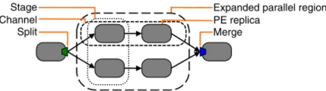
Parts of the stream graph that the compiler determines are safe to parallelize are called unexpanded parallel regions, as shown in Fig. 2. Note that the compiler only demarcates where the parallel regions are; it does not transform the stream graph. The runtime performs the graph transforma-tion, producing the expanded parallel region at job submission time, as shown in Fig. 3.

Besides auto-parallelization, another important streaming optimization is fusion [4], [12]. Fusion combines multiple operators into a single PE (processing element) to reduce communication overhead. PEs become operating system pro-cesses. Our compiler ensures that PEs never span parallel region boundaries. PEs in the same application execute simultaneously, potentially on separate hosts. Operators inside of a PE communicate through function calls and shared memory; operators in different PEs communicate through TCP over the network. Because our runtime is distributed, we must carefuly consider what information to communicate across PEs.

The runtime expands the parallel regions by replicating their PEs. A port is the point where a PE and a stream connect. The runtime implements split as a special output port, and merge as a special input port. We refer to each path through an expanded parallel region as a channel. The set of replicas of the same PE is called a stage. These are illustrated in Fig. 3.

3

COMPILER

The compiler’s task is to decide which operator instances belong to which parallel regions. Furthermore, the compiler picks implementation strategies for each parallel region, but not the degree of parallelism. One can think of the compiler as being in charge of safety while avoiding platform-dependent profitability decisions.

3.1 Safety Conditions

This section lists sufficient pre-conditions for auto-parallelization. As usual in compiler optimization, our approach is conservative: the conditions may not always be necessary, but they imply safety. The conditions for paralleliz-ing an individual operator instance are:

No state or partitioned state: The operator instance must be either stateless, or its state must be a map where the key is a set of attributes from the input tuple. Eachfiring only updates the state for the given key. This makes it safe to parallelize by giving each operator replica a disjoint partition of the key domain.

At most one predecessor and successor: The operator instance must have fan-in and fan-out . This means parallel

Stage Channel Split

Expanded parallel region PE replica

Merge

Fig. 3. Stream graph, from the runtime’s perspective. Processing element (PE)

Unexpanded parallel region Operator instance

Stream

Fig. 2. Stream graph, from the compiler’s perspective.

2. In our runtime, operators maintain a map from keys to their associ-ated state. Operators obtain keys by hashing the values of the attributes from the partitioning set. So, given a state map, a current tuple and the set of partitioning attributes {a1 an}, each operator firing accesses:

regions have a single entry and exit where the runtime can implement ordering.

The conditions for forming larger parallel regions with multiple operator instances are:

Compatible keys: If there are multiple stateful operator instances in the region, their keys must be compatible. A key is a set of attributes, and keys are compatible if their intersection is non-empty. Parallel regions are not re-quired to have the exact same partitioning as the opera-tors they contain so long as the region’s partitioning key is formed from attributes that all operators in the region are also partitioned on. In other words, the partitioning cannot degenerate to the empty key, where there is only a single partition. It is safe to use a coarser partitioning at the parallel region level because it acts as first-level routing. The operators themselves can still be partitioned on afiner grained key, and that finer grained routing will happen inside the operator itself.

Forwarded keys: Care must be taken that the region key as seen by a stateful operator instance indeed has the same value as at the start of the parallel region. This is because the split at the start of the region uses the key to route tuples, whereas uses the key to access its partitioned state map. All operator instances along the way from the split to must forward the key unchanged; i.e., they must copy the attributes of the region key unmodified from input tuples to output tuples.

Region-local fusion dependencies: SPL programmers can influence fusion decisions with pragmas. If the pragmas require two operator instances to be fused into the same PE, and one of them is in a parallel region, the other one must be in the same parallel region. This ensures that the PE replicas after expansion can be placed on different hosts of the cluster.

No shuffle after prolific regions: A shuffle is a bipartite graph between the end of one parallel region and the beginning of the next. A prolific region is a region containing prolific operators, i.e., operators that can emit multiple output tuples for a single input tuple. Prolifacy causes tuples with duplicate sequence numbers. Within a single stream, such tuples are still ordered. But after a shuffle, this ordering could be lost. Thus, the compiler does not allow a shuffle at the end of a prolific region.

3.2 Compiler Analysis

This section describes how the compiler establishes the safety conditions from the previous section. We mustfirst distin-guish an operator definition from an operator invocation. The operator definition is a template, such as an Aggregate oper-ator. It provides different configuration options, such as what window to aggregate over or which function (Count, Avg, etc.) to use. Since users have domain-specific code written in C++ or Java, we support user-defined operators that encap-sulate such code. Each operator definition comes with an operator model describing its configuration options to the compiler. The operator invocation is written in SPL and con-figures a specific instance of the operator, as shown in Fig. 1. The operator instance is a vertex in the stream graph.

We take a two-pronged approach to establishing safety: program analysis for operator invocations in SPL, and properties in the operator model for operator definitions. This is a

pragmatic approach, and requires some trust: if the author of the operator deceives the compiler by using the wrong properties in the operator model, then our optimization may be unsafe. This situation is analogous to what happens in other multi-lingual systems. For instance, the Java keyword final is a property that makes a field of an object immutable. However, the author of the Java code may be lying, and actually modify thefield through C++ code. The Java com-piler cannot detect this. By correctly modeling standard library operators, and choosing safe defaults for new opera-tors that can then be overridden by their authors, we dis-charge our responsibility for safety.

The followingflags in the operator model support auto-parallelization. The default for each is Unknown.

state Stateless ParamPartitionBy Unknown .

In the ParamPartitionBy case, the partitionBy pa-rameter in the operator invocation specifies the key.

selectivity ExactlyOne ParamFilter

AtMostOne ParamGroupBy Unknown .

Using consumption to production ratios, selectivity (ExactlyOne) means 1:1, selectivity (AtMostOne) means

and Unknown selectivity means . In the

ParamFiltercase, the selectivity is if there is a Filter

parameter, and otherwise. In the ParamGroupBy case,

the selectivity is Unknown if there is a groupBy parameter, and otherwise3_.

forwarding Always FunctionAny Unknown .

In the Always case, all attributes are forwarded unless the operator invocation explicitly changes or drops them. The FunctionAnycase is used for aggregate operators, which forward only attributes that use an Any function in the operator invocation.

In most cases, analyzing an SPL operator invocation is straightforward given its operator model. However, operator invocations can also contain imperative code, which may affect safety conditions. State can be affected by mutating expressions such as n or foo n , if function foo modifies its parameter or is otherwise stateful. SPL’s type system supports the analysis by making parameter mutability and statefulness of functions explicit [9], similar to Finifter et al. [13]. Selectivity can be affected if the operator invocation calls submit to send tuples to output streams. Our compiler uses data-flow analysis to count submit-calls. If submit-calls appear inside of -state-ments, the analysis computes the minimum and maximum selectivity along each path. If submit-calls appear in loops, the analysis assumes that selectivity is Unknown.

3.3 Parallel Region Formation

After the compiler analyzes all operator instances to deter-mine the properties that affect safety, it forms parallel regions. In general, there is an exponential number of possible choices, so we employ a simple heuristic to pick one. This leads to a faster algorithm and more predictable results for users.

Our heuristic is to always form regions left-to-right. In other words, the compiler starts parallel regions as close to 3. In SPL, filter parameters are optional predicates that determine when to drop tuples, and groupBy parameters cause a separate output tuple for each group.

sources as possible, and keeps adding operator instances as long as all safety conditions are satisfied. This is motivated by the observation that in practice, more operators are selective than prolific, since streaming applications tend to reduce the data volume early to reduce overall cost. Therefore, our left-to-right heuristic tends to reduce the number of tuples travel-ing across region boundaries, where they incur split or merge costs. Our heuristic assumes that the partitioning key space is not skewed. If it is, then the optimal decision must also minimize the number of operators exposed to the skew, which our heuristic may not do.

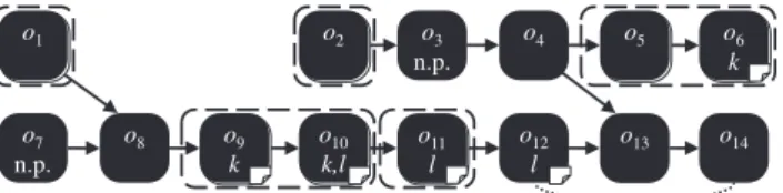
The example stream graph in Fig. 4 illustrates our algo-rithm. The first parallel region contains just , since its successor violates the fan-in condition. Similarly, the next region contains just , since its successor is“n.p.” (not parallelizable). Operator instances and are combined in a single region, since is stateless and has state partitioned

by key . The region with and ends before , because

adding would lead to an empty region key. This illustrates our left-to-right heuristic: another safe alternative would have been to combine with instead of . Finally, is not in a parallel region, because it has a fusion dependency with (recall that programmers can request operators to be fused together into a PE). That means they would have to be in the same parallel region, but is in the way and violates the

fan-in condition.

3.4 Implementation Strategy Selection

Besides deciding which operator instances belong to which parallel region, the compiler also decides the implementation strategy for each parallel region. We refer to the single entry and single exit of a region as the first joint and last joint, respectively. Thefirst joint can be a parallel source, split, or shuffle. Likewise, the last joint can be a parallel sink, merge, or shuffle. The compiler decides the joint types, as well as their implementation strategies. Later, the runtime picks up these decisions and enforces them.

Our region formation algorithm keeps track of the region key and overall selectivity as it incrementally adds operator instances to the region. When it is done forming a region, the compiler uses the key to pick a tuple-routing strategy (e.g., hashing), and it uses the selectivity to pick an ordering strategy (for example, round-robin). After region formation, the compiler inserts shuffles between pairs of adjacent parallel regions, and adjusts their joint types and ordering strategies accordingly.

3.5 Interaction with Fusion

As mentioned before, besides the auto-parallelization optimi-zation, the SPL compiler supports an auto-fusion optimization.

On top of that, users can influence fusion decisions with pragmas. The compiler first checks the pragmas to infer mandatory fusion dependencies between operator instances. Next, it runs the region-formation algorithm, which updates the stream graph with unexpanded parallel regions. Finally, the compiler runs the fusion algorithm, which updates the stream graph with PEs, as shown in Fig. 2.

We modified the fusion algorithm to ensure that it respects region-safety conditions. Specifically, if the auto-parallelizer decides to put two operator instances into different parallel regions, then the auto-fuser must put them into different fused PEs. SPL’s fusion algorithm works by iterative refinement [12]. In the original version, it starts with a single PE contain-ing all operator instances, and then keeps dividcontain-ing PEs into smaller ones to introduce task and pipeline parallelism. In our modified version, instead of starting from a single PE, the algorithm starts from one PE per region, plus one PE for all operator instances that are not part of any region. Then, it iteratively refines starting from those PEs.

4

RUNTIME

The runtime has two primary tasks: route tuples to parallel channels, and enforce tuple ordering. Parallel regions should be semantically equivalent to their sequential counterparts. That equivalence is maintained by ensuring that the same tuples leave parallel regions in the same order regardless of the number of channels.

The distributed nature of our runtime—PEs can run on separate hosts—has influenced every design decision. We favored a design which does not add out-of-band communi-cation between PEs. Instead, we either attach the extra infor-mation the runtime needs for parallelization to the tuples themselves, or add it to the stream.

4.1 Splitters and Mergers

Routing and ordering are achieved through the same mechan-isms: splitters and mergers in the PEs at the edges of parallel regions (as shown in Fig. 3). Splitters exist on the output ports of the last PE before the parallel region. Their job is to route tuples to the appropriate parallel channel, and add any information needed to maintain proper tuple ordering. Mer-gers exist on the input ports of thefirst PE after the parallel region. Their job is to take the streams from each parallel channel and merge their tuples into one, well-ordered output stream. The splitter and merger must perform their jobs invisibly to the operators both inside and outside the parallel region.

4.2 Routing

Tuple routing is orthogonal to tuple ordering. When parallel regions only have stateless operators, the splitter routes tuples in round-robin fashion. When parallel regions have parti-tioned state, the splitter is not free to route any tuple to any channel: the channels will have accumulated state based on the attributes they expect. The splitter uses the attributes that define the partition key to compute a hash value. It then uses that hash to route the tuple, ensuring that the same attribute values are always routed to the same operators.

o8 o7 n.p. o3 n.p. o4 o12 l o13 o14 o1 o9 k o10 k,l o2 o11 l o5 o6 k

Fig. 4. Parallel region formation example. Operator instances labeled “n.p.” are not parallelizable (e.g., due to unknown state). The letters and indicate key attributes. The dotted line from to indicates a fusion dependency. Dashed ovals indicate unexpanded parallel regions. The paper icons indicate stateful operators.

4.3 Ordering

There are four different ordering strategies: round-robin, sequence numbers, and strict vs. relaxed sequence numbers. (We define pulses in Section 4.3.3.) The situations in which each strategy is employed depend on state and selectivity, as shown in Table 1.

Internally, mergers maintain queues for each channel. PEs work on a push basis. So a PE can receive tuples from a channel even if the merger is not yet ready to send them downstream. The queues let the merger accept tuples from the transport layer immediately and handle them later as dictated by their ordering strategy.

In fact, all of the merging strategies follow the same algo-rithm when they receive a tuple. Upon receiving a tuple from the transport layer, the merge places that tuple into the appropriate queue. It then attempts to drain the queues as much as possible based on its ordering strategy. All of the tuples in each queue are ordered. If a tuple appears ahead of another tuple in the same channel queue, then we know that it must be submitted downstream first. Mergers, then, are actually performing a merge across ordered sources. Several of the ordering strategies take advantage of this fact. 4.3.1 Round-Robin

The simplest ordering strategy is round-robin, and it can only be employed with parallel regions that have stateless opera-tors with a selectivity of 1. Because there is no state, the splitter has the freedom to route any tuple to any parallel channel. On the other end, the merger can exploit the fact that there will always be an output tuple for every input tuple. Tuple ordering can be preserved by enforcing that the merger pops tuples from the channel queues in the same order that the splitter sends them.

The left side of Fig. 5 shows an example of a round-robin merge. The merger has just received a tuple on channel 1, which is next in the round-robin order, so the merger submits the tuple on queue 1, followed by the front tuples on queues 2 and 0, and again waits on 1.

4.3.2 Sequence Numbers

The second ordering strategy is sequence numbers, where the splitter adds a sequence number to each outgoing tuple. The PE runtime inside of each parallel channel is responsible for ensuring that sequence numbers are preserved; if a tuple with sequence number x is the cause of an operator sending a tuple, the resulting tuple must also carry x as its sequence number. When tuples have sequence numbers, the merger’s job is to submit tuples downstream in sequential order.

The precondition for using sequence numbers without pulses is selectivity 1: 1, i.e., every sequence number shows

up at the merger exactly once, without omissions or dupli-cates. Therefore, the merger can submit a tuple with number nextwhen the gap between lastSeqNo and next is 1. The merger maintains lastSeqNo and a minimum-heap nextHeapof the channel queue heads. While the top of the nextHeaphas a gap of 1, the merger drains and submits it.

This is a heap operation, where is the number of

channels. The following function determines if a sequence number is ready to be submitted:

def gap seqno :

return seqno lastSeqno

def readySeqno next :

return gap next 1

The second pane of Fig. 5 shows an example of a sequence number merge that has just received a tuple on channel 1. The merger uses the nextHeap to keep track of the lowest se-quence number across all channel queues. In this instance, it knows that lastSeqno 4, so the next tuple to be submit-ted must be 5. The top of the nextHeap is 5, so it is submitsubmit-ted. Tuples 6 and 7 are also drained from their queues, and the merger is then waiting for 8.

4.3.3 Strict Sequence Number and Pulses

A more general strategy is strict sequence number and pulses, which permits operators with selectivity at most 1, meaning they may drop tuples. In that case, if the last tuple to be submitted was y, the merger cannot wait until y 1 shows up—it may never come. But timeouts are inappropriate, since our system is designed for arbitrarily sized computations.

Pulses solve this problem. The splitter periodically sends a pulse on all channels, and the length of this period is an epoch. Pulses carry the same sequence number on all channels, and pulses are merged along with tuples. Operators in parallel channels forward pulses regardless of their selectivity; even an operator that drops all tuples will still forward pulses. The epoch limits the memory requirements for the channel queues at the merger, or conversely, prevents deadlock if the channel queues are bounded-size buffers [14].

The presence of pulses guarantees that the merger will receive information on all incoming channels at least once per epoch. The merger uses pulses and the fact that all tuples and pulses come in sequential order on a channel to infer when a tuple has been dropped. In addition to the nextHeap, the merger maintains an additional minimum-heap of the tuples last seen on each channel, which are the backs of the channel queues. This heap keeps track of the minimum of the max-imums; the back of each channel queue is the highest sequence number seen on that channel, and the top of this heap is the minimum of those. We call this heap the seenHeap. It makes finding the min-of-the-maxes a operation. Consider the arrival of the tuple with sequence number z. As in the

sequence number case, if z lastSeqno 1 where

lastSeqnois the sequence number of the tuple submitted last, then z is ready to be submitted. If that is not the case, we may still submit z if we have enough information to infer that tuple z 1 has been dropped. The top of the seenHeap can provide that information: if 1is less than the top of the seenHeap, then we know for certain that z 1 is never coming, since all channels have moved on to higher sequence numbers already. Recall that the top of the seenHeap is the TABLE 1

lowest sequence number among the backs of the channel queues (the min-of-the-maxes), and that the channel queues are in sequential order.

Using the above reasoning, we can define a function that determines whether we can infer that a particular sequence number has been dropped:

def dropped seqno :

return seqno < seenHeap top and isSteadyState The function isSteadyState returns true only if we have received a tuple on each channel, and false otherwise. Establishing that we have some information on every channel is critical, as without it, we cannot conclude that a tuple has been dropped.

Because establishing that a sequence number has been dropped requires being in the steady state, we cannot deter-mine that a tuple has been dropped at startup. Hence, we still want to pay attention to sequential order, as in the sequence number case. Using the already defined functions, then the condition for strict sequence number and pulses is:

def readyStrictSeqnoAndPulse next :

return gap next 1_{or dropped next 1}

In other words, we can submit next if it is next in strict sequential order, or if we can establish that next 1 has been dropped.

The third pane of Fig. 5 shows an example of a strict sequence number and pulses merger that has just received a tuple on channel 1. In addition to the nextHeap, the merger uses the seenHeapto track the lowest sequence number among the backs of the queues. In this instance, lastSeqno 4, so the merger needs to either see 5 or be able to conclude it is never coming. After 8 arrives on channel 1 and becomes the top of the seenHeap, the merger is able to conclude that 5 is never coming—the top of the seenHeap is the lowest sequence number of the backs of the queues, and < . The merger then submits 6, and it also has enough information to submit 8. It cannot submit 10 because it does not have enough information to determine if 9 has been dropped.

4.3.4 Relaxed Sequence Number and Pulses

The prior merge strategies are sufficient only in the absence of prolific operators—operators where a single firing can pro-duce > tuples. Our system handles prolific operators by giving the same sequence number to all tuples in a group. So, if an operator consumes a tuple with sequence number x, all of the tuples produced as a result of thatfiring will also have sequence number x. We call such sequence numbers duplicates. The merger must be able to handle duplicates, yet still maintain correct ordering. The challenge in handling dupli-cates is making certain that the merger has seen all duplidupli-cates for a particular sequence number before submitting higher sequence numbers. The manner in which we establish this fact

is similar to establishing that a tuple has been dropped: we monitor the backs of the channel queues, looking for evidence that it is impossible for a particular sequence number to arrive.

We are aided this time by the fact that if sequence number x arrives on channel c, then duplicates of x can only arrive on the same channel c. If we can establish that a sequence number greater than x arrived on channel c, then it is impossible for the merger to receive any more duplicates of x. Thus, we only need to check the queue for the last channel we received a tuple on, which we keep track of with lastChan. Using that reasoning, we can define a function which performs this check:

def noDups seqno :

return seqno channels lastChan back

When the merger wants to evaluate if sequence number s is in order, it also has to check if it can prove that there are no outstanding duplicates for s 1. Until the merger can prove that no more tuples with sequence number s 1 will arrive, it cannot be sure that submitting s will be in sequential order. However, the presence of duplicates means that it is possible for the gap between s and lastSeqNo to be 0—they are the same. In that case, it is clearly ready to be submitted. Thefinal decision to submit a tuple is then expressed as:

def readyRelaxedSeqnoAndPulse next :

return gap next 0

or gap next 1and noDups next 1

or gap next > 1 and dropped next 1 In other words, we can submit next if there is no gap between it and the last sequence number submitted (they are the same); or, if the gap is 1, then we can submit it if we can prove that no duplicates for next 1 can arrive; or we can submit next if the gap is greater than 1, and we can prove that

next 1has been dropped.

The far right of Fig. 5 shows an example of a relaxed sequence number and pulses merge. The seenHeap is not yet usable (shown as a dangling pointer), because we have yet to receive a tuple or pulse on channel 1. The top of the nextHeapis 5, and lastSeqno 1 is 5, so we can establish that the top of the nextHeap is in relaxed (non-decreasing) order. However, we must also be able to prove that no more tuples can arrive with sequence number 4. Since a tuple with sequence number 4 last arrived on channel 0, and we can see that the back of channel 0’s queue is 7, we can prove that no more duplicates of 4 will arrive because < . We can then submit 5, but we are unable to subsequently submit 7 because it is still possible for duplicates of 5 to arrive on channel 2.

4.4 Shuffles

When the compiler forms parallel regions (Section 3.3), it aggressively tries to merge adjacent regions. Adjacent parallel regions that are not merged are sequential bottlenecks. When next 0 1 2 nextHeap 0 1 2 7 10 13 6 9 12 15 lastSeqno = 4 nextHeap 0 1 2 10 16 22 6 12 18 24 lastSeqno = 4 5 8 seenHeap

Round-Robin Sequence Numbers Strict Sequence Number & Pulses

nextHeap 0 1 2 7 7 7 5 lastSeqno = 4 lastChan = 0 seenHeap

Relaxed Sequence Number & Pulses 7

channels channels

channels channels

possible, the compiler merges parallel regions by simply re-moving adjacent mergers and splitters. Section 3.1 lists the safety conditions for when merging parallel regions is possible. However, when adjacent parallel regions have incompatible keys, they cannot be merged. Instead, the compiler inserts a shuffle: all channels of the left parallel region end with a split, and all channels of the right parallel region begin with a merge. Shuffles preserve safety while avoiding a sequential bottleneck. In principle, shuffles are just splits and merges at the edges of adjacent parallel regions. However, splits and merges in a shuffle modify their default behavior, as shown in Fig. 6.

Ordinary splitters have both routing and ordering respon-sibilities. The ordering responsibility for an ordinary splitter is to create and attach sequence numbers (if needed) to each outgoing tuple. When tuples arrive at a splitter in a shuffle, those tuples already have sequence numbers. The PE itself preserves sequence numbers, so a splitter in a shuffle only has routing responsibilities. Splitters inside of a shuffle also do not generate pulses; they were already generated by the splitter at the beginning of the parallel region.

When mergers exist at the edge of parallel regions, they are responsible for stripping off the sequence numbers from tuples and dropping pulses. Mergers that are a part of a shuffle must preserve sequence numbers and pulses. But they cannot do so naively, since mergers inside of a shuffle will actually receive copies of every pulse, where is the number of parallel channels. The split before them has to forward each pulse it receives to all of the mergers in the shuffle, meaning that each merger will receive a copy of each pulse. The merger prevents this problem from exploding by ensuring that only one copy of each pulse is fowarded on through the channel. If the merger did not drop duplicated pulses, then the number of pulses that arrived at thefinal merger would be on the order of where is the number of stages connected by shuffles.

5

PUNCTUATIONS

Punctuations are control signals in a stream that are interleaved with tuples [9]. Punctuations impact auto-parallelization, including both compile-time region formation and run-time policy enforcement. Before we detail how our auto-parallelizer handles punctuations, we briefly discuss what they are, how they are used in our system, and the set of composition rules governing the interaction of punctuations with operators.

5.1 Punctuation Kinds

Our system uses three kinds of punctuations. First are window punctuations, which are one of the ways to create windows within a stream. Such windows identify a group of tuples that form a larger unit. For instance, a group of tuples marked by

window punctuations can be reduced as a batch using an aggregate operator. Second arefinal punctuations, which iden-tify the end of a stream. While streams are potentially infinite, in practice they do terminate when applications are brought down. Final punctuations help implementing logic associated with termination processing, such as flushing buffers. The third kind of punctuations are pulses, as described in Sec-tion 4.3.3. Unlike the other punctuaSec-tions, pulses never exist outside of a parallel region.

5.2 Punctuation Rules

We now look at the rules that govern operator composition under punctuations. An output port of an operator can either generate, remove, or preserve punctuations. Punctuation-free output ports guarantee that their output stream does not contain punctuations, whereas punctuation-preserving ports will forward punctuations from the input (if they exist). An input port of an operator can either be punctuation-oblivious or punctuation-expecting. An input port is oblivious to punc-tuations if it does not require a punctuated stream to function properly, whereas punctuation-expecting input ports must be connected to exactly one punctuated stream.

A stream is punctuated if it is generated by a punctuation-generating output port or an output port that preserves punctuations from an input port that receives a single punc-tuated stream. Performing fan-in on two puncpunc-tuated streams results in a stream that is not punctuated, since punctuation semantics are lost (e.g., window boundaries are garbled).

5.3 Region Formation and Punctuations

We now describe how punctuation rules impact parallel region formation. Operators with punctuation-expecting in-put ports depend on up-stream operators that generate punc-tuated streams and forward them (if any). If a down-stream operator depends on punctuations generated or forwarded from an up-stream operator , and is in a parallel region, then must be in the same parallel region as . Otherwise, the replicas of would each independently generate punc-tuations, which would have undefined semantics for .

In summary, during region formation, the compiler en-sures that if an operator is inside a parallel region, then other operators that have punctuation dependencies on it are also inside the same parallel region. If this causes other conflicts, then the operator cannot be placed in a parallel region.

5.4 Runtime Handling of Punctuations

The punctuation safety checks performed by the compiler prevent punctuations generated from inside a parallel region from ever reaching a merger. However, punctuations gener-ated by an operator outside and before a parallel region are allowed to pass through the region. Unlike tuples, punctua-tions do not carry unique data. Rather, they are semantic markers inside of a stream, and for that reason, punctuations must be routed to all channels inside of a parallel region.

Because punctuations are duplicated at the split, the merg-er has to take care not to submit the duplicated punctuations downstream. For the round-robin ordering strategy, the merge recognizes when it is submitting a punctuation, and it knows that the next full round of items to submit will be duplicates of that punctuations. The merger checks that they are and drops them.

H1 F0 Src F1 F₂ H0 H₂ Sink

creates, attaches seqnos; creates, sends pulses

forwards seqnos, pulses

G1

G0

G2

removes seqnos; drops pulses

forwards seqnos; receives N pulses, forwards 1 Fig. 6. Splitter and merger responsibilities in a shuffle.

When tuples have sequence numbers, handling duplicate punctuations is actually easier. The splitter assigns the same sequence number to all duplicates of a punctuation. When a punctuation is a candidate for submitting downstream, the merger checks its sequence number. If the sequence number is less than or equal to the last-submitted sequence number, then the punctuation is a duplicate and the merger drops it. This behavior is the same as for pulses.

6

RESULTS

We use three classes of benchmarks. The scalability bench-marks are designed to show that simple graphs with data parallelism will scale using our techniques. Our microbe-nchmarks are designed to measure the overhead of runtime mechanisms that are necessary to ensure correct ordering. Finally, we use five application kernels to show that our techniques can improve the performance of stream graphs inspired by real applications.

All of our experiments were performed on machines with 2 Intel Xeon processors where each processor has 4 cores with hyperthreading. In total, each machine has 8 cores, 16 threads, and 64 GB of memory. Each machine runs Linux, with a 2.6 version of the kernel.

Our Large-scale experiment uses 112 cores across 14 ma-chines. The large-scale experiments demonstrate the inherent scalability of our runtime, and indicate that the linear trends seen in the other experiments are likely to continue. The machines in the large-scale experiments were connected with Ethernet. The remainder of our experiments use 4 machines connected with Infiniband.

Our experiments in Sections 6.1 and 6.2 vary the amount of work per tuple on the -axis, where work is the number of integer multiplications performed per tuple4. We scale this exponentially to explore how our system behaves with both very cheap and very expensive tuples. When there is little work per tuple, scaling is harder because the parallelization overhead is significant compared to the actual work. Hence, the low end of the spectrum—the left side of the -axis—is more sensitive to runtime parallelization overheads. The high end of the spectrum—the right side of the -axis—shows the scalability that is possible when there is sufficient work.

All data points in our experiments represent the average of at least three runs, with error bars showing the standard deviation.

6.1 Scalability Benchmarks

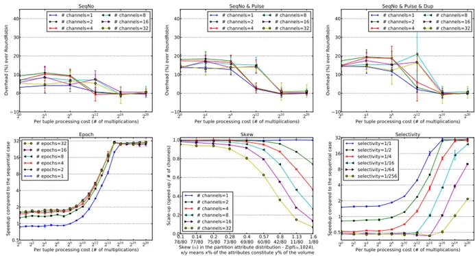
The scalability benchmarks, Fig. 7, demonstrate our runtime’s scalability across a wider range of parallel channels. These experiments use 4 machines (32 cores). When there is a small amount of work per tuple (left side of the -axis), these experiments also show how sensitive the runtime is to having more active parallel channels than exploitable parallelism.

The Stateless scalability experiment has a stream graph with a single stateless operator inside of a parallel region. Because the operator in the parallel region is stateless, the compiler recognizes that the runtime can use the least expen-sive ordering strategy, round-robin. Hence, we observe linear scalability, up to 32 times the sequential case when 32 parallel channels are used with 32 cores available. Just as importantly, when there is very little work—when the amount of work to be done is closer to the parallelization cost—additional paral-lel channels do not harm performance.

The stream graph is the same for the Stateful scalability experiment, but the operator is an aggregator that has local state. The compiler instructs the runtime to use sequence numbers and pulses to ensure proper ordering. The scalability is linear for 2–16 parallel channels, and achieves 31.3 times the sequential case for 32 parallel channels when using 32 cores. However, all cases see some performance improvement with very inexpensive work, with all but the 32-channel cases never dropping below improvement. The 32-channel case never has less than improvement for very inexpensive work. This result indicates that our runtime has little overhead. Note that in the Stateful experiment, inexpensive work exhibits more than improvement for 1–8 channels, which is not the case with the Stateless experiment. Even though the per-tuple cost is the same for both experiments, the aggregation itself adds afixed cost. Hence, operators in the Stateful experi-ment do more work than operators in the Stateless experiexperi-ment. Very inexpensive work in the Stateful experiment is benefiting from both pipeline and data parallelism.

Fig. 8 shows the stream graph for the Shuffle experiment, which has two aggregations partitioned on different keys, requiring a shuffle between them. When there are 32 channels in the Shuffle experiment, there are actually 64 processes (two Fig. 7. Scalability benchmarks.

Aggr Aggr Src Aggr Aggr Aggr Aggr Sink 1 1 1 1 1 1

Fig. 8. Expanded stream graph for a two-way shuf_fle. 4. The parallelized operator uses integer multiplications as a way to

PEs per channel) running on 32 cores. (In the Stateless and Stateful experiments, 32 channels use only 32 processes: one PE per channel.) Hence, the 32-channel case is an over-subscribed system by a factor of 2, and it only scales to . The 16-channel case has 32 PEs, which is a fully subscribed system, and it scales to . As with the Stateful experiment, the inexpensive end of the work spectrum ben-efits from pipeline as well as data parallelism, achieving over

improvement for 4–32 channels.

Note that the effect of pipeline parallelism for low tuple costs is least pronounced in the Stateless experiment, and most pronounced in Shuffle. In the sequential case with low-tuple costs, the one PE worker is the bottleneck; it must receive, process, and send tuples. The splitter only sends tuples. As the number of parallel channels increases, the work on each worker PE decreases, making the splitter the bottleneck. The more costly the work is, the stronger the effect becomes, which is why it is weakest in the Stateless experiment and strongest in the Shuffle experiment.

The Large-scale experiment in Fig. 10 demonstrates the scalability the runtime system is able to achieve with a large number of cores across many machines. This experiment uses a total of 14 machines. One machine (8 cores) is dedicated to the source and sink, which includes the split and merge at the

edges of the parallel region. The other 13 machines (104 cores) are dedicated to the PEs in the parallel region. The stream graph for the stateful experiment is a single, stateful aggrega-tion in a parallel region with 100 parallel channels. The stateful experiment shows near linear scalability, maxing out at improvement.

The shuffle experiment in Fig. 10 has the same stream graph as shown in Fig. 8. Therefore, there are twice as many processes as parallel channels. When there are 50 parallel channels in each of its two parallel regions, the improvement

in throughput maxes out at . The shuffle experiment

cannot scale as high as stateful because with 50 parallel channels, there are 100 PEs.

6.2 Microbenchmarks

Fig. 9 shows the microbenchmarks. The stream graph for the microbenchmarks is a single-operator parallel region.

As described in Section 4.3, adding sequence numbers to tuples and inserting pulses on all channels will incur some overhead. We measured this overhead in Fig. 9, using pure round-robin ordering as the baseline. As expected, as the work-per-tuple increases, the cost of adding a sequence num-ber to each tuple becomes negligible compared to the actual work done. However, even when relatively little work is done, the highest average overhead is only 12%. Pulses add more overhead, but never more than 21%. As with sequence numbers alone, the overhead goes towards zero as the cost of the work increases. Handling duplicates due to prolific re-gions does not add extra overhead on top of pulses, but results in slightly higher variance in the overhead results.

Epochs, as explained in Section 4.3, are the number of tuples on each channel between generating pulses on all channels. The Epoch experiment in Fig. 9 measures how sensitive performance is to the epoch length. An epoch of means that the splitter will send tuples, where is the number of channels, before generating a pulse on each

– – –

Fig. 9. Microbenchmarks.

channel. We scale the epoch with the number of channels to ensure that each channel receives tuples before it receives a single pulse. The default epoch is . Results show that beyond an epoch length of 8, speedup does not vary more than 8% in the range from 8–32.

The Skew experiment in Fig. 9 demonstrates that because our runtime does not yet perform dynamic load balancing, it may be vulnerable to skewed distributions in parallel regions with partitioned state. As explained in Section 4.2, when parallel regions contain partitioned state, tuples are routed based on a hash of the key attributes. Hence, each tuple has a particular channel it must be routed to. The -axis is the amount of skew. The first data point on the -axis means that 78% of the keys constitute 80% of the volume, in other words, there is only very little skew. The last data point on the -axis means that 1% of the attributes constitute 80% of the volume. As expected, when many tuples must be routed to a few channels, speedup suffers. This experiment indicates that our runtime could benefit from dynamic load balancing. While the runtime is unable to change the fact that a particular tuple must be routed to a single channel, it could separate out the heavily loaded attributes into different channels.

In the Selectivity experiment, we fixed the number of parallel channels at 32. Each line in the graph represents a progressively more selective aggregator. So, when selectivity is 1:1, the operator performs an aggregation for every tuple it receives. When selectivity is 1:256, it performs 1 aggregation for every 256 tuples it receives. When per-tuple cost is low, and the selectivity increases, the worker PEs do very little actual work; they mostly receive tuples. However, the cost for the splitter remains constant, as it always has 32 channels. When selectivity is high, the splitter is paying the cost to split to 32 channels, but there is no benefit to doing so, since real work is actually a rare event. As a result, as selectivity increases, there is actually slowdown until the cost of proces-sing one of the selected tuples become large.

The Punctuation experiment in Fig. 11 quantifies the impact of punctuated streamsflowing through parallel regions. As explained in Section 5.4, punctuations are replicated on all channels. As the number of punctuations increases, the inher-ent data parallelism decreases. The -axis varies the amount of punctuations per tuple in a stream. On the left, at 1, there is 1 punctuation for every tuple. On the far right, at 256, there is 1 punctuation for every 256 tuples.

As expected, when the stream has many punctuations, the overhead is high: there is no data parallelism to exploit, but we still pay all of the synchronization overheads. The only exception is for the largest tuple processing cost, for which

the extra cost of having a punctuation for every tuple is negligible. As the number of punctuations in the stream decreases, the performance approaches the same as in the Stateless scalability benchmark.

6.3 Application Kernels

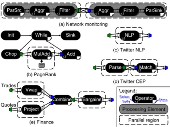
This section further explores performance using five real-world application kernels shown in Fig. 12. All of these application kernels have selective or stateful parallel regions, which require the techniques presented in this paper to be parallelized.

The Network monitoring kernel monitors multiple servers, looking for suspicious user behavior. The filters remove values below a“suspicious” threshold. The left parallel region is partitioned by the server, while the right parallel region is partitioned by users, with a shuffle in the middle. Note, however, that because there are parallel sources on the left and parallel sinks on the right, tuples are not ordered in this application. The compiler recognizes this and informs the runtime that it has only routing responsibilities.

The PageRank kernel uses a feedback loop to iteratively rank pages in a web graph [15]. This application is typically associated with MapReduce, but is also easy to express in a streaming language. Each iteration multiplies the rank vector with the web graph adjacency matrix. In thefirst iteration, MulAddreads the graph from disk. Each iteration uses the parallel channels of MulAdd to multiply the previous rank vector with some rows of the matrix, and uses Add to assemble the next rank vector. The input consists of a synthetic graph of 2 million vertices with a sparsity of 0.001, in other words, 4 billion uniformly distributed edges.

The Twitter NLP kernel uses a natural language processing engine [16] to analyze tweets. The input is a stream of tweet contents, and the output is a list of tuples containing the words used in the message, their lengths, and their frequencies. The stream graph has a parallel region with a single, stateless, prolific operator. The NLP engine is implemented in Java, so tuples that enter the NLP operator must be serialized, copied into the JVM, processed, then deserialized and copied out of the JVM.

The Twitter CEP kernel uses complex event processing to detect patterns across sequences of tweets [17]. The Parse Fig. 11. Punctuation overhead.

Parse Match Vwap Project Combine Bargains Trades Quotes MulAdd Add Chop While Sink Init

ParSrc Aggr Filter Aggr Filter ParSink

NLP

(a) Network monitoring

(b) PageRank (c) Twitter NLP (d) Twitter CEP (e) Finance Operator Processing Element Parallel region Legend: ≤1 ≤1 ≤1 ≤1 ≤1 ≥1 ≤1 ≤1 Selec-tivity State

operator turns an XML tweet into a tuple with author, con-tents, and timestamp. The Match operator detects sequences offive consecutive tweets by the same author with identical hash-tags. This pattern is a pathological case for this input stream, which causes thefinite state machine that implements the pattern matching to generate and check many partial matches for most tuples. Both Parse and Match are paralle-lized, with a shuffle to partition by author before Match. The topology is similar to that of the Network monitoring kernel, but since there is no parallel source or sink, ordering matters.

The Finance kernel detects bargains when a quote exceeds the VWAP (volume-weighted average price) of its stock symbol. The graph has three parallelizable operators. Only the Combine operator, which merges its two input streams in timestamp order, is not parallel.

Fig. 13 shows the parallel speedups of thefive application kernels on a cluster of 4 machines with 8 cores each, for a total of 32 cores. In these experiments, all parallel regions are replicated to the same number of parallel channels. For example, when the number of channels is 32, Twitter CEP has a total of 64 operator instances, thus over-subscribing the cores. Most of the kernels have near-perfect scaling up to 8 channels. The exception is Finance, which tops out at a

speed-up of with 4 channels, at which point the Combine

operator becomes the bottleneck. The other application ker-nels scale well, topping out at either 16 or 32 chanker-nels, with

speedups between and over sequential.

Table 2 shows the average time it takes for all operators in parallel regions to process tuples. The average timings in-cludes a mix of integer and floating point operations that could potentially include cache misses and branch mispredictions.

7

RELATED

WORK

The StreamIt compiler auto-parallelizes operators using round-robin to guarantee ordering [4]. The StreamIt language supports stateful and dynamic operators, but StreamItfission only works for stateless operators with static selectivity. We treat it as a special case of our more general framework, which also fisses operators with partitioned state and dynamic selectivity. Furthermore, unlike StreamIt, we support more general topologies that eliminate bottle-necks, including par-allel sources, shuffles, and parpar-allel sinks.

To achieve our scaling results for stateful operators, we adapt an idea from distributed databases [18], [19]: we parti-tion the state by keys. This same technique is also the main factor in the success of the MapReduce [20] and Dryad [21]

batch processing systems. However, unlike parallel data-bases, MapReduce, and Dryad, our approach works in a streaming context. This required us to invent novel techniques for enforcing output ordering. For instance, MapReduce uses a batch sorting stage for output ordering, but that is not an option in a streaming system. Furthermore, whereas parallel databases rely on relational algebra to guarantee that data parallelism is safe, MapReduce and Dryad leave this up to the programmer. Our system, on the other hand, uses static analysis to infer sufficient safety preconditions.

There are several efforts, including Hive [22], Pig [23] and FlumeJava [24], that provide higher-level abstractions for MapReduce. These projects provide a programming model that abstracts away the details of using a high performance, distributed system. Since these languages and libraries are abstractions for MapReduce, they do not work in a streaming context, and do not have the ordering guarantees that our system does. Efforts on making batch data processing systems more incremental include MapReduce Online, which reports approximate results early [25], and the Percolator which allows observers to trigger when intermediate results are ready [26]. Unlike these hybrid systems, which still experience high latencies, our system is fully streaming.

Spark Streaming is a stream processing framework de-signed to deal with fault tolerance and load balancing in a distributed system [27]. The model, called discretized streams, divides a continuous streaming computation into stateless, deterministic transformations on batches. These transformations are inherently data parallel, as they are state-less and apply to distributed data sets. However, Spark Streaming does not enforce ordering on their records, nor does it have to do any analysis to determine if a transforma-tion can be parallelized.

Storm is an open-source project for distributed stream computing [3]. The programming model is similar to ours— programmers implement asynchronous bolts which can have dynamic selectivity. Developers can achieve data parallelism on any bolt by requesting multiple copies of it. However, such data parallelism does not enforce sequential semantics; safety is left entirely to the developers. S4 is another open-source streaming system [2], which was inspired by both MapReduce and the foundational work behind Streams [28]. In S4, the runtime dynamically instantiates replica PEs for each new value of a key. Creating replica PEs enables data parallel-ism, but S4 has no mechanisms to enforce tuple ordering. Again, safety is left to developers.

There are extensions to the prior work on data-flow par-allelization that are complementary to our work. River [29] and Flux [30], part of the adaptive query processing line of work, perform load-balancing for parallelflows. Both of these leave safety to developers. Microsoft StreamInsight uses a Fig. 13. Performance results for the application kernels.

TABLE 2