MODELING
THE OFFICER RECRUITMENT
AND
MANPOWER PLANNING PROCESS
IN TURKISH LAND FORCES
A THESIS
SUBMITTED TO THE DEPARTMENT OF INDUSTRIAL
ENGINEERING
AND THE INSTITUTE OF ENGINEERING AND SCIENCES
OF BILKENT UNIVERSITY
IN PARTIAL FULFILLMENT OF THE REQUIREMENTS
FOR THE DEGREE OF MASTER SCIENCE
By
Arz Pekmezci
August, 2001
I certify that I have read this thesis and that in my opinion it is fully adequate, in scope and in quality, as a thesis for the degree of Master of Science.
Asst. Prof. Oya Ekin Karaşan (Principal Advisor)
I certify that I have read this thesis and that in my opinion it is fully adequate, in scope and in quality, as a thesis for the degree of Master of Science.
Assoc. Prof. Mustafa Ç. Pınar
I certify that I have read this thesis and that in my opinion it is fully adequate, in scope and in quality, as a thesis for the degree of Master of Science.
Asst. Prof. Yavuz Günalay
Approved for the Institute of Engineering and Sciences
Prof. Mehmet Baray
ABSTRACT
MODELING THE OFFICER RECRUITMENT AND MANPOWER PLANNING PROCESS IN TURKISH LAND FORCES
Arz Pekmezci
M. S. In Industrial Engineering Supervisor : Asst. Prof. Oya Ekin Karaşan
August 2001
The objective of this study is to improve the Turkish Land Forces officer accessions and manpower planning process. A model for planning officer accessions to Turkish Land Forces from sources that have different characteristics is presented. This model takes into account factors such as attritions, involuntary retirements, promotions and transitions to determine the impact of existing policies over the long term and to determine adjustments that might be required to reach authorized strength goals. The annual supply of accessions necessary to meet the strength goal with minimum deviations is determined. This manpower planning model is created using the modeling software GAMS.
ÖZET
TÜRK KARA KUVVETLERİNDE SUBAY ALIMI VE İNSANGÜCÜ PLANLAMASI İŞLEMİ MODELLEMESİ
Arz Pekmezci
Endüstri Mühendisliği Bölümü Yüksek Lisans Tez Yöneticisi : Yrd. Doç. Dr. Oya Ekin Karaşan
Ağustos 2001
Bu çalışmanın amacı, Türk Kara Kuvvetlerinde subay alımı ve insan gücü planlama işleminin geliştirilmesidir. Değişik özelliklere sahip kaynaklardan Türk Silahlı Kuvvetlerine subay tedariki planlaması modeli sunulmaktadır. Bu model, ayrılmalar, mecburi emeklilik, terfiler ve geçişler gibi faktörleri dikkate alarak uzun vadede mevcut personel politikasının etkisini inceler ve kadro hedeflerine ulaşmak için gerekli değişiklikleri belirler. En az sapmalarla kadro hedeflerine ulaşmak için ihtiyaç duyulan yıllık giriş teminine karar verir. Bu insan gücü planlaması modeli GAMS modelleme yazılımı kullanılarak oluşturulmuştur.
ACKNOWLEDGEMENT
I am very grateful to my supervisor Dr. Oya Ekin Karaşan for her guidance, patience, encouragement and understanding in each phase of the study.
I am thankful to Dr. Mustafa Ç. Pınar and Dr. Yavuz Günalay for accepting to read and review this thesis.
I would like to thank Major Adnan Bıçaksız for his corrections in a very limited time and Captain Levent Biber for his understanding and support during the collection of data.
I would like to thank all Industrial Engineering faculty, staff and my friends for their assistance and support during the graduate study.
Finally, I am very thankful to my family for their support, tolerance and patience during every stage of my life.
Contents
1.
Introduction and Review
1
1.1 The Concepts of the Manpower Planning
1
1.2 The Goal of the study
2
1.3
Literature Review
3
2.
Characteristics of The Turkish Land Forces
Personnel System
8
2.1 Personnel Categorization
8
2.2 Ranks
8
2.3 Sources
13
2.3.1 Military Academy 13
2.3.2 Non-Commissioned Officers (Type 1) 13 2.3.3 Non-Commissioned Officers (Type 2) 14 2.3.4 Conscripted Reserve Officers 15
2.3.5 Civilian Accessions 15
2.3.6 Contract Officers 15
2.4 Branches
16
2.5 The Current Manpower Planning Model
17
3. Mathematical Formulation and Analysis of the
Problem
19
3.1 Indices
20
3.2 Initial Data and Parameters
22
3.4 Constraints
27
3.4.1 Attrition constraints 27 3.4.2 Transition constraints 28 3.4.3 Inventory constraints after attritions and transitions 29 3.4.4 Promotion constraints 29 3.4.5 Non-promotion constraints 31 3.4.6 Accession constraints 32 3.4.7 Capacity constraints 34 3.4.8 Inventory constraints 34 3.4.9 Rank constraints 38 3.4.10 Balance constraints 39 3.4.11 Deviation constraints 40 3.4.12 Objective Function 40
3.5 Experimentation
40
3.6 Scenario Analysis
42
4. Conclusions
48
4.1 Decision Support System
48
4.2 Future Work
49
APPENDICES
A.
The accessions for original scenario
53
B.
The percentage deviations for original scenario
65
C.
The accessions for alternative scenario
77
D.
The percentage deviations for alternative scenario
89
E.
Anglo-Turkish Glossary Military Terms
101
List of Figures
3.1 The general figure of the process for combat arms 45 3.2 The general figure of the process for non-combat arms 46 3.3 The recruitment process according to sources and years of
List of Tables :
2.1 The periods of the ranks for commissioned officers 9 2.2 The station ceilings (original) for commissioned officers 10 2.3 The station ceilings (revised) for commissioned officers 10 2.4 The matching of ranks and category cohorts 11 2.5 The rates of normal and early promotions 12 2.6 The distribution of NCOs by years of service at the time of transition to officer (Type 1) 14 2.7 The distribution of NCOs by years of service at the time of transition to officer (Type 2) 15
2.8 The list of Combat arms 17
2.9 The list of Non-Combat arms 17 3.1 The normalization of the authorized strength goals 23 3.2 The factors given to negative and positive deviations 24 3.3 The weights given to negative deviations 25 3.4 The weights given to positive deviations 25 3.5 Minimum required time to reach ranks 42 3.6 The alternative periods of ranks 43 3.7 The costs of original and alternative scenarios 44
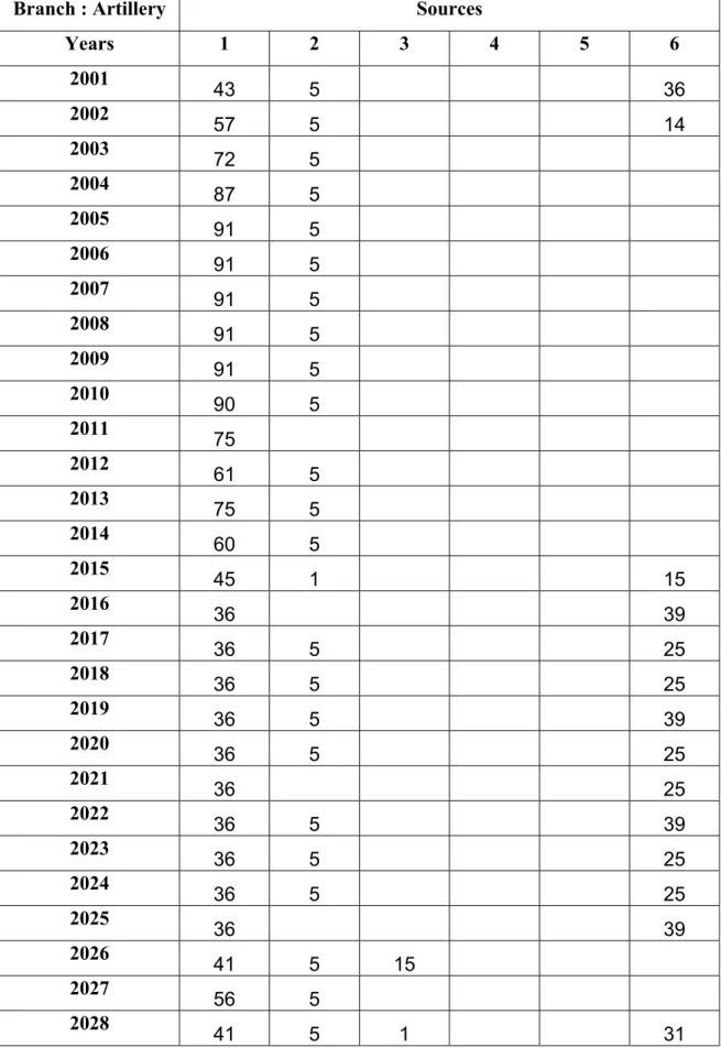
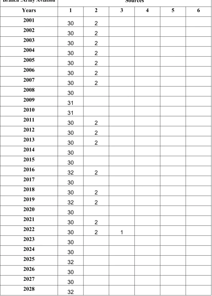
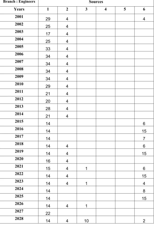
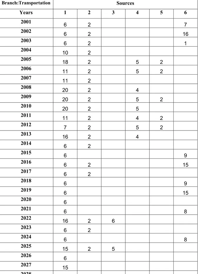
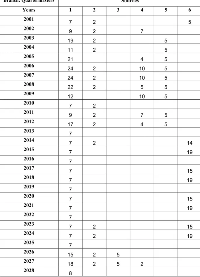
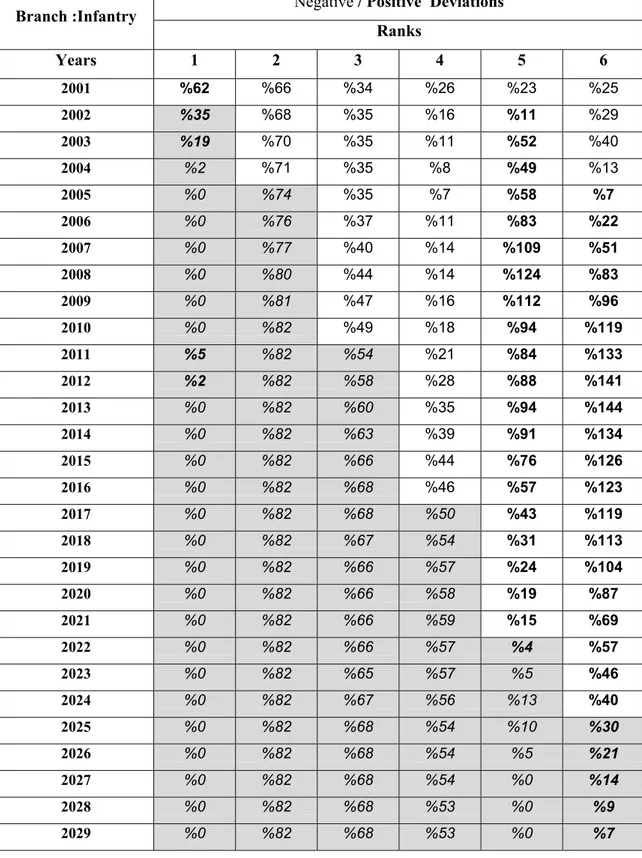
A.3 The number of accessions for Artillery 55 A.4 The number of accessions for Air Defense 56 A.5 The number of accessions for Army Aviation 57 A.6 The number of accessions for Signals 58 A.7 The number of accessions for Engineers 59 A.8 The number of accessions for Ordnance 60 A.9 The number of accessions for Transportation 61 A.10 The number of accessions for Personnel 62 A.11 The number of accessions for Quartermasters 63 A.12 The number of accessions for Finance 64 B.1 The percentage deviations for Infantry 65 B.2 The percentage deviations for Armor 66 B.3 The percentage deviations for Artillery 67 B.4 The percentage deviations for Air Defense 68 B.5 The percentage deviations for Army Aviation 69 B.6 The percentage deviations for Signals 70 B.7 The percentage deviations for Engineers 71 B.8 The percentage deviations for Ordnance 72 B.9 The percentage deviations for Transportation 73 B.10 The percentage deviations for Personnel 74 B.11 The percentage deviations for Quartermasters 75 B.12 The percentage deviations for Finance 76 C.1 The number of accessions for Infantry 77 C.2 The number of accessions for Armor 78 C.3 The number of accessions for Artillery 79
C.4 The number of accessions for Air Defense 80 C.5 The number of accessions for Army Aviation 81 C.6 The number of accessions for Signals 82 C.7 The number of accessions for Engineers 83 C.8 The number of accessions for Ordnance 84 C.9 The number of accessions for Transportation 85 C.10 The number of accessions for Personnel 86 C.11 The number of accessions for Quartermasters 87 C.12 The number of accessions for Finance 88 D.1 The percentage deviations for Infantry 89 D.2 The percentage deviations for Armor 90 D.3 The percentage deviations for Artillery 91 D.4 The percentage deviations for Air Defense 92 D.5 The percentage deviations for Army Aviation 93 D.6 The percentage deviations for Signals 94 D.7 The percentage deviations for Engineers 95 D.8 The percentage deviations for Ordnance 96 D.9 The percentage deviations for Transportation 97 D.10 The percentage deviations for Personnel 98 D.11 The percentage deviations for Quartermasters 99 D.12 The percentage deviations for Finance 100
CHAPTER 1
INTRODUCTION and REVIEW
1.1 Concepts of the Manpower Planning
Stainer [18] describes the aim of manpower planning as to maintain and improve the ability of the organization to achieve corporate objectives, through the development of strategies designed to enhance contribution of manpower at all times in the foreseeable future.
According to Bennison and Casson [1] the manpower planning’s framework involves three steps:
"
1. Estimate the organization’s future manpower needs in terms of the numbers of people required of different skills and occupations at all levels in the organization. 2. The means by which the organization will meet these needs are now examined. In
other words, how is the manpower to be supplied? To arrive at the supply the levels of wastage must be studied, the rate at which people progress through the organization must be studied, and an attempt must be made to quantify the labor markets from which the recruits are drawn.
3. The gap between the needs and the supply should now be evident. Where there are insufficient people of the required ability to fill promotions, other sources of manpower must be investigated. Transfers from other parts of the organization, recruitment of experienced people directly from outside, possibly the promotion of good people from lower levels than normal; all are possible means of closing the gap. At this stage the basic levels of recruitment necessary for the organization to cover its leavers and meet its overall demand for manpower can be determined. Sometimes these calculations show that the wastage levels are not great enough to reduce the number of staff to the overall demand and the organization has to consider redundancy policies. "
Linear programming, markov and renewal models have been designed to help understand and predict the interrelated movements of employees by promotion, recruitment, transfer, and wastage within, to and from a system.
In manpower planning process, the basic factors affecting the decision process are: - the level of demand
- the rate of attrition from the system - the replacement policy
- the promotion policy
In manpower planning process, there are two types of flow; those within the system and those between the system and the environment. The major internal flows are :
- promotions - nonpromotions - transitions
The major flows into and out of the system are: - recruitment
- attrition (resignation, voluntary retirement, discharge, death) - involuntary retirement
1.2 The goal of the study
To meet the officer demand in Turkish Land Forces, there are some projects underway. The authorized strength goal is the number officers required in a rank for each branch, during peace time. The aim of our study is to analyze the current manpower planning system of the Turkish Land Forces and to determine required adjustments for better meeting the authorized strength goal by taking into consideration some critical factors such as attritions, promotions, involuntary retirements,
non-Turkish Land Forces need a new: -efficient -flexible -reliable -optimized -standardized -computer assisted
manpower planning process. Also, the new system should - include all relevant criteria,
- permit application of a flexible promotion system, - facilitate application of alternative personnel policies, - facilitate comparison of the alternatives.
This study has the scope of:
- Analyzing current personnel accession and flow model - Modeling the accession and flow process
- Improving the personnel flow model by adding new criteria or modifying existing criteria
- Determining and applying a convenient goal programming algorithm
- Determining the alternative periods of ranks to achieve the authorized strength goal better.
1.3 Literature Review
Manpower planning first appeared after the turn of the century and especially in 1960’s it has received much attention. The initial manpower planning process concentrated on the problems of effective utilization of manpower on the shop floor. The establishment of the system and techniques in the 1960’s moved the study of planning into office systems. Then, manpower planning has turned to the behavior of individuals since individuals with high motivation make great contribution to the
system’s effectiveness. Hence it is very important to motivate the individuals by supplying them with objectives and goals by emphasizing the necessity of the individual to the achievement of the organization goals and by offering careers that are fair and reasonable.
In 1969, A NATO conference was organized about the manpower planning studies in the military area and the following papers are cited from this conference:
Charnes et al. [3] developed a model for civilian manpower management and planning in the U.S. Navy. The model aims to improve the processes of manpower planning for the U.S. Navy by means of computer assisted mathematical models that combine goal programming and Markov transition processes.
Cotteril [5] developed a simple static model for forecasting officer requirements. The method was employed in the Canadian Forces to calculate what the structure would be if an assumed set of personnel policies were to persist for a long period of time, giving a position of equilibrium. This model helps the personnel manager to examine many more sets of policy options under more sets of assumed conditions than when he had to make these calculations by hand.
Forbes [8] presented a study on the promotion and recruitment policies for the control of quasi-stationary hierarchical systems. This study is a discrete Markov chain model with classes corresponding to the category cohort or age classes of a manpower system.
Lindsay [13] developed a computerized system for projection of long-range military manpower accession requirements and manpower supply. This system permits alternative manpower policies to be evaluated very quickly as requirements, estimated gains and attritions and costs vary.
In 1978, Grinold [19] developed an equilibrium model of a manpower system based on the notion of a career flow. Institutional constraints and measures of system performances are linear functions of the career flow. The optimization problem is a generalized linear program in which columns are generated by solving a shortest path problem.
In 1980, Bres et al. [2] developed a goal programming model for planning officer accessions to the U.S. Navy from various commissioning sources. Present and future requirements for different career branch areas in the Navy are considered in terms of years of commissioned service and related to various choke points where inventories fall short of requirements in officer structure.
In 1980, Holz and Wroth [12] presented a study on improving strength forecasts for army manpower management. It is the military manpower program which contains forecasts of strength, gains, and attritions over a seven-year period, based on both historical time-series data and projected effects of changes in policy and other conditions.
In 1983, Collins et al. [4] developed “The Accession Supply Costing and Requirement Model (ASCAR)” to evaluate the accession needs of the All Volunteer Armed Forces to reach or maintain a given strength and optimize the qualitative mix of new recruits. It uses goal programming and allows the analyst to simulate and analyze the effects of manpower policy and program changes or the size and the composition of the enlisted active duty forces.
In 1986, Holloran and Byrn [11] developed United Airlines station manpower planning system for scheduling shift work at its reservation offices and airports. The system utilizes integer and linear programming and network optimization techniques and encompasses the entire scheduling process from forecasting of requirements to printing employee schedule choices.
In 1988, Gass et al. [10] developed the Army Manpower Long-Range Planning System (MLRPS) that provides the analytical capability to project the strength of the
active U.S. Army for 20 years. The model simulates the interaction of gains, attritions, promotions and retypes to enable the analyst to determine the impact of existing policies over long term, and to determine changes that might be required to reach a desired force.
McClean [14] presented a study on manpower planning models and their estimation which is concerned with models which seek to describe the various manpower flows and the estimation techniques which have been developed in conjunction with these models. It concentrates on the practicalities of describing the entire manpower system and predicting its future development. In particular, it focuses on the use of a Markov chain formulation which implements the mathematically intractable semi-Markov approach by means of a non-parametric estimation procedure.
In 1995, Durso and Donahuel [7] presented an analytical approach to reshaping the U.S. Army, “The Total Army Personnel Life Cycle Model (TAPLIM)”. This model analyzes the impacts on the U.S. Army’s enlisted force of key personnel management policies to meet congressional requirements and support a changing national military strategy. Its versatility and flexibility enhanced a strategic personnel process designed to reshape the US army.
In 1995, Reeves and Reid [16] presented a study on a military reserve manpower planning model. It is a multiple objective model for manpower planning in a company sized military reserve unit. Given resource limitations and the conflicting nature of the objectives, it is not possible to achieve all model objectives completely. So in the study, the reserve officers are used as subjects to participate in a process to identify preferred efficient model solutions interactively.
In 2000, Çandar [6] studied on a goal programming model for promotion system in the Turkish army. It proposed a flexible promotion system that aims to fill job positions with the purpose of incorporating performance criteria. This study is developed and
Our study differentiates from the work of Çandar [6] in the following subjects : 1. His study aims to reach the authorized strength goals by promotion rates and
assumes that the number of officer accessions to branch armor is constant. The number of officer accessions to any branch is not fixed in real world dynamics. It is determined by the military manpower analyst based on the current personnel policy. Hence, in our study, we used the current promotion rates and aimed to reach the authorized strength goals by the number of officer accessions.
2. We developed and analyzed the model for all branches and include the interaction of branches, i.e. transitions from the combat arms to non-combat arms.
3. The differences among officers from different sources are inserted to the model. This is a necessity since officers follow different career paths according to their sources.
4. An alternative policy for the periods of ranks is proposed at the end of our study to improve the manning ratio of the authorized strength goals.
CHAPTER 2
THE CHARACTERISTICS OF THE TURKISH
LAND FORCES PERSONNEL SYSTEM
2.1 Personnel Categorization
The Turkish Army consists of six personnel categories that are commissioned officers (referred to as “officers”), non-commissioned officers (NCOs), specialists, conscripted reserve officers (CROs), enlisted corps, and civilians. Officers, NCOs and specialists make up the Army professionals in uniform. Officers are career soldiers and make up the managerial cadres in the Army. Non-commissioned officers (NCOs) are also career soldiers and make up the lower management cadres or technical cadres of the Army depending on their trades. Specialists are recruited for 2- or 3-year contracts for specific job positions that require expertise and make up the shop-floor foremen or supervisors as those present in the industry. The hierarchical structure, job positions, career paths, sources, basically, all the personnel policies for the officers and non-commissioned officers vary. In this study, we deal with the recruitment and flow model of the officers, the members of the highest hierarchical category in the Turkish Land Forces.
2.2 Ranks
The hierarchical structure of the officers in the army is maintained with a total of six ranks that are from the lowest to the highest:
1. Second Lieutenant 2. First Lieutenant 3. Captain
The officers in the first three ranks are called junior officers, and the officers in the remaining three ranks are called senior officers.
An officer starts his service in the army with the rank of a Second Lieutenant and can not leave the service until the completion of 15 years obligatory service, and can retire from the army after 18 years of service. To promote to the next rank, an officer should serve in the current rank for a certain duration, which is called “the period of rank”. The periods of ranks are as shown in Table 2.1.
Table 2.1 : The periods of ranks for commissioned officers
After the officer completes the period of rank for the colonel rank, he is retired automatically unless promoted to the rank of a brigadier. Since the whole system is different for general officers, they are not in the scope of this study.
There exist some criteria for each rank that force an officer who has not been promoted for a certain period to leave the army. The maximum time that an officer can wait in the same rank is determined by the Law No.926 Armed Forces Personnel Law. These are called as station ceilings in the military literature as shown in Table 2.2.
RANKS PERIODS OF RANKS
Second Lieutenant 3 Years First Lieutenant 6 Years Captain 6 Years
Major 5 Years
Lieutenant Colonel 3 Years Colonel 5 Years
Table 2.2 : The station ceilings (original) for commissioned officers
Individuals who reach the station ceiling are retired from the army automatically. To express the station ceilings in the same unit of measure, we consulted with the military manpower analyst in the Army HQ, and then transformed the age criteria for the first two ranks into years of service and obtained the station ceilings in the same unit of measure as shown in Table 2.3.
Table 2.3 : The station ceilings (revised) for commissioned officers
In military literature, each year of the period of a rank is called "the category cohort". RANKS STATION CEILINGS
Second Lieutenant 41 years old First Lieutenant 46 years old Captain 21 years of service Major 25 years of service Lieutenant Colonel 27 years of service Colonel 31 years of service
RANKS STATION CEILINGS Second Lieutenant 19 years of service First Lieutenant 21 years of service Captain 21 years of service Major 25 years of service Lieutenant Colonel 27 years of service Colonel 31 years of service
RANKS PERIODS CATEGORTY COHORTS
1 2 Second Lieutenant 3 years
3 4 5 6 7 8 First Lieutenant 6 years
9 10 11 12 13 14 Captain 6 years 15 16 17 18 19 Major 5 years 20 21 22 Lieutenant Colonel 3 years
23 24 25 26 27 Colonel 5 years 28 Table 2.4 : The matching of ranks and category cohorts
The station ceilings are the factors which determine retirement process in ranks. However, in rank Colonel, there is an exception. The officers who reach the last category cohort (28), are retired from the army whatever their years of service are. The officers whose years of service become greater than station ceiling of rank Colonel (31 years) are also retired before reaching the last category cohort. Basically, the officers who reach the last category is taken out of the system next year.
Under current conditions, every rank has a period to be completed. When an officer completes the period of rank, he typically promotes to the next rank. Without completing the full required period of rank, it is possible for officers in some ranks (First Lieutenant, Captain, Major) to promote to the next rank with the rate of early promotion. The rates of normal and early promotions according to category cohorts can be seen in Table 2.5.
Combat Arms Non-Combat Arms Category
Cohorts Rate of normal promotion Rate of early promotion Rate of normal promotion Rate of early promotion 8 0.92 0.08 0.96 0.04 14 0.92 0.08 0.96 0.04 19 0.92 0.08 0.96 0.04
• The rates of normal promotions for other category cohorts that are not mentioned in the table, are one.
• The rates of early promotions for other category cohorts that are not mentioned in the table, are zero.
Table 2.5: The rates of normal and early promotions
possible only from the category cohort which is just prior to the last, for ranks, First Lieutenant, Captain, Major.
As it can be understood from the table, the total promotion rate from any category cohort is one, that means the officers promote each year. However, there are exceptions depending on sources of the officers which will be explained in the following section.
2.3 Sources
The Turkish Land Forces acquire officers from six sources which have different capacities and characteristics. The officers from all sources start to work in the first category cohort of rank Second Lieutenant. The sources are the Military Academy, NCOs (type 1), NCOs (type 2), conscripted reserve officers, civilian accessions, and contract officers.
2.3.1. Military Academy
The main source of the army is the military academy. Most of the cadets in the military academy come from the military high schools. A small amount of the cadets are civilian students who graduate from a regular high school and pass a special exam administered by the army. In the last few years, female students are taken to the military academy and they are educated in the same conditions and chances as males. The military academy can provide officers for all branches which we shall analyze.
2.3.2. Non-Commissioned Officers (Type 1)
The non-commissioned officers (NCOs) form another professional category of the army. To motivate the NCOs, there is a career path opportunity to continue their service life as officers. The NCO who graduates from a university takes a military exam and according to the demand and the exam’s result, he may be commissioned as a Second Lieutenant. An officer from this source can lead to the rank of a Colonel. NCOs with a service time of 7 to 12 years may apply for transition up to the commissioned officer
category. NCOs` previous years of service should be taken into account. To accommodate this, we used the rates of NCO transition to officer with regard to years of service which are calculated previously by a research group in Army HQ. Table 2.6 shows the distribution of NCO transitions to officer by their years of service at the time of transition:
Table 2.6: The distribution of NCOs by years of service at the time of transition to officer (Type 1)
2.3.3 Non-Commissioned Officers (Type 2)
The NCOs who have outstanding performance in the army have chances to become officers. Even though a university degree is not required, a military exam must be taken. According to the exam results, demand and previous performance evaluations, some of the NCOs may become officers. However, they can not promote beyond the rank of a captain as opposed to Type 1 transitions. Also they can not have early promotions.
NCOs with a service time of 7 to 9 years may apply for transition up to the commissioned officer category. As done for Type1 NCOs, we used the rates of NCO
Years of Service as NCO at the time of transition
Percent of All NCO transitions in the same group
7 10 % 8 20 % 9 20 % 10 20 % 11 20 % 12 10 %
Table 2.7 : The distribution of NCOs by years of service at the time of transition to officer (Type 2)
2.3.4 Conscripted Reserve Officers (CROs)
The CROs after completing their obligatory service in the army can apply to become officers. According to their performance evaluations and demand, some of them are then accepted to the army as officers.
2.3.5 Civilian Accessions
Any person who has graduated from a university can apply to join and to serve in the army as an officer. According to their professional areas, the applications are screened and the potential candidates are offered to take an exam. Based on the exam results and demand, some may be accepted to the army as officers.
2.3.6 Contract Officers (COs)
In the near future, the personnel policy of the army is to become more professional and well-trained. Hence, recruitment by contract is legislated to implement this policy.
In the long run, the CROs will be replaced by contract officers. The contract term is 3 years. At the end of this period, the contract can be renewed for another 3-year term or
Years of Service as NCO at the time of transition
Percent of All NCO transitions in the same group
7 40 %
8 30 %
can be cancelled depending upon both parties’ wishes. The officers from this source can not have early promotions.
Briefly, the sources have different characteristics. For example the officers from source NCO (Type 2) and contract officers cannot promote beyond the rank of a captain. Also the officers from the contract officers source can leave the army or can be fired from the army or continue their duties with a new contract only at the end of 3 years period. Since an NCO has served in the army before becoming an officer, the total service period in the army as an NCO is taken into account in the model whereas an officer from the other sources enters the model with only 1 years of service.
Even if it seems inconsistent to achieve the authorized strength goals, the personnel policy of the army necessitates that, the military academy should graduate a fixed number of officers for each branch every year, whatever the strength goal of the branch is.
2.4
Branches
The Turkish Land Forces have a number of branches. We shall only deal with the branches that are valid for newly-graduated military academy officers. As a consequence of military tactics, the branches can be divided into two groups :
1. Combat arms: Those which actually conduct war in the battlefield (Table 2.8). 2. Non-Combat arms: Those which support the combat arms in various ways (Table
Table 2.8 : The list of Combat arms
Table 2.9 : The list of Non-Combat arms
Because of the necessity of a professional army, it is preferred to provide the demand of the combat arms only from the military academy, NCOs (both types) and COs.
2.5 The Current Manpower Planning Model
The current accession and flow model of officers is primarily based on the analyst’s intuition. There exist some accumulation factors for each rank and branch. The analyst enters the possible accessions from the sources to obtain the manning ratio by the accumulation factors and see the future inventory and then analyzes the results. If necessary, he enters the new accessions according to the results of the previous analysis.
Combat Arms 1. Infantry 2. Armor 3. Artillery 4. Air Defense 5. Army Aviation 6. Signals 7. Engineers Non-Combat Arms 1. Ordnance 2. Transportation 3. Personnel 4. Quartermasters 5. Finance
After repeating this process and analyzing the results, the analyst reaches a "solution". As it can be understood, this process highly depends on the analyst’s capability and point of view. It is reviewed every 2 years to get more accurate results.
The process focuses primarily on achieving the authorized strength goal of senior officers (Major, Lieutenant Colonel, Colonel). There are some problems about the manning ratios especially in the authorized strength goals of senior officer ranks. Negative deviation (less than desired) causes some job positions that can not be filled through the reserved personnel to be filled with the officers that are in subordinate ranks. Positive deviation (more than desired) in senior officer ranks, however, is completely an undesirable situation for the army.
CHAPTER 3
MATHEMATICAL FORMULATION
and
ANALYSIS OF THE PROBLEM
As with all large-scale mathematical modeling, it is important to determine that the model has been described properly in the computer based system, that the resulting mathematical description is a proper and acceptable representation of the real world problem, and that solutions obtained from the model can be implemented in practice. In each step of the study, the manpower analysts in the headquarters of the army analyzed the phase and directed the study to represent real world dynamics. The solution of the study will be analyzed by the authorized personnel and will then be proposed to the army for implementation.
Because of the size of the problem and GAMS capacity, we can not solve the problem which includes all branches in one model. Hence, we separate the problem into 2 pieces, one for combat arms, called phase 1, and one for non-combat arms, called phase 2. Solving the problem in two phases does not cause any loss of generality, since
- The combat arms have no interaction among themselves and so do non-combat-arms. There exist interaction among branches only by the transitions from combat arms to non-combat arms. In order to take care of this interaction, we calculated the transition-out variables from combat arms to non-combat arms in phase 1, then inserted these variables as transition-in parameters, for non-combat arms.
- The officers in branches acquire from six sources. It may be thought that since they come from the same sources, the capacity of sources would be a problem. However, every source has upper and lower capacities that are marked for each branch separately. Hence there is no problem with regard to sources.
We should observe that the nature of the problem necessitates solving first phase 1 and then phase 2.
Phase 1 :
This phase consists of solving the manpower planning process for the combat arms. Transitions between the branches can be generalized as one-way flow from combat arms to non-combat arms. The officers of combat arms whose medical conditions no longer allow them to serve in these branches are transferred into the non-combat arms. Phase 2 :
This phase consists of solving the manpower planning process for non-combat arms. The transition-out variables that are found at the end of phase 1 are entered into the model as the transition-in parameters in phase 2.
To set the stage for the discussion that follows, we illustrate the aspects of the manpower planning model .
3.1 Indices
T: Set of calendar years S: Set of category cohorts R: Set of ranks
I : Set of branches J: Set of sources
K: Set of years of service N: Set of non-combat arms
Calendar Years t = 2001,2002,...,2029 Category Cohorts s = 1,2,...,28
Branches i = Infantry, Armor, Artillery, Air Defense, Army Aviation, Signals, Engineers (only used in Phase 1)
Branches i = Ordnance, Transportation, Personnel, Quartermasters, Finance (only used in Phase 2)
Sources j= Military Academy, NCOs (Type 1), NCOs (Type 2), CROs, Civilian, COs
Years of service k = 1,2,...,31
Non-Combat Arms n= Ordnance, Transportation, Personnel, Quartermasters, Finance (only used in phase 1)
In mathematical formulation of the model, we have the following assumptions : - The Contract officers do not leave the army in anyway during their contracts. - The officer accessions from all sources occur at the same time.
- The rates of attrition and transition are predetermined.
In the model, in spite of the maximum years of service to be 31 years (station ceiling of rank Colonel), the maximum duration of service as an officer, i.e. no early promotions, is 28 years. The officers from sources military academy, CROs, Civilian, enter the model with years of service 1 and reach the last category cohort at the end of 28 years. The officers from source COs , again, enter the model with years of service 1 and promote to the rank of a captain and stay there until the station ceiling of this rank is completed. The station ceiling of captain rank is 21 years, hence they can remain in the system maximum 21 years. The officers from source NCO (Type1) enter the model with years of service between 7 and 12, and can move up to the rank of a Colonel. The officers from this source, who will stay in the system maximum period are the ones with the smallest years of service (7). They reach the station ceiling of rank Colonel (31 years) after 25 years, so they stay in the system maximum for 25 years. The officers from source NCO (Type2) enter the model with years of service between 7 and 9, and promote to the rank of a captain and stay there until the station ceiling of the rank is
completed. The station ceiling of rank Captain is 21 years, hence they can remain in the system maximum for 14 years. Therefore, to see the full affect of the model, it is enough to run the model for 28 years. Observe that the initial inventory (2001) is given and we start the model from the end of 2001.
As mentioned in Chapter 2, the ranks are divided into 28 category cohorts to accommodate for the year in each rank. Since the officers have different career behavior according to their sources, we define 6 sources. We define years of service 1 to 31 years, since the maximum years of service in the army can be 31 years.
In phase 1, we define 7 combat arms. There exists some transitions from combat arm to non-combat arms because of deterioration of medical conditions and to show these transitions, the non-combat arms should be defined in phase 1.
In phase 2, there is no transition-out process for the non-combat arms, hence it is enough to define just 5 non-combat arms.
3.2 Initial Data and Parameters
Mv(i,s,j,k) Given initial inventory for branch i, category cohort s, source j, with years of service k, in 2001
Capu(i,j) Upper capacity of source j, for branch i Capl(i,j) Lower capacity of source j, for branch i D(i,r) Strength goal of branch i, in rank r
Rpro(s) Normal promotion rate for category cohort s Rbpro(s) Early promotion rate for category cohort s
Rtrano(i,s,n) Rate of transition-out from branch i (combat arms), to branch n (non-combat arms), for category cohort s ( used in Phase 1)
The required data such as strength goals, attrition rates, promotion rates for each rank and military branch is taken from the headquarters of the Turkish Land Forces. The authorized strength goals for each rank of every branch are the ideal numbers of the army during peace time. The rates are determined after a comprehensive statistical study that is undertaken by a research group in the army.
Wn(i,r) Weight given to negative deviation (shortfall) for branch i and rank r Wp(i,r) Weight given to positive deviation (surplus) for branch i and rank r
The authorized strength goals of ranks are different and hence we should normalize them before calculating the weights. The normalization of the authorized strength goals for each rank of every branch can be seen in Table 3.1.
Branches Second. Lieut.
First
Lieut. Capt. Maj.
Liet. Col. Col. Infantry 9.35 1 2.38 4.86 18.78 13.65 Armor 7.12 1 1.63 2.94 10.3 7.49 Artillery 5.72 1 1.37 2.45 5.19 5.55 Air Defense 9.3 1 2.08 3.64 8.4 17.6 Army Aviation 5.92 1 1.49 2.63 13.82 11.2 Signals 7.32 1 1.38 2.98 7.87 5.32 Engineers 7.09 1 1.49 2.67 5.37 6.7 Ordnance 6.68 1 1.02 2.1 3.87 4.48
Transportation 4.49 1 1.54 2.1 4.4 4.4
Personnel 5.64 1 1.02 1.4 2.4 2.4
Quartermasters 5.94 1 1.02 1.58 3.3 3.4
Finance 5.3 1.3 1 1.2 1.87 1.32
Table 3.1 : The normalization of the authorized strength goals
After normalization of the authorized strength goals, we determined the factors that are given one unit negative and positive deviation for each rank of every branch by using the following logic. The authorized strength of senior officers has higher priority, the factors for them should be larger than the junior officers. On the other hand, an officer can serve in a job position marked for an officer superior in rank, but cannot serve in a job position marked for an officer subordinate in rank. Hence the factor given to negative deviation should be larger than the factor given to positive deviation. The factors can be seen in Table 3.2.
Table 3.2 : The factors given to negative and positive deviations
Finally, to calculate the weights given to negative and positive deviations, we Ranks Factor for Neg. Dev. Factor for Pos. Dev.
Second Lieutenant 1 3 First Lieutenant 1 3 Captain 2 4 Major 5 8 Lieutenant Colonel 6 9 Colonel 7 10
Branches Second. Lieut.
First
Lieut. Capt. Maj.
Liet. Col. Col. Infantry 9,35 1 4,76 24,3 112,68 95,55 Armor 7,12 1 3,26 14,7 61,8 52,43 Artillery 5,72 1 2,74 12,25 31,14 38,85 Air Defense 9,3 1 4,16 18,2 50,4 123,2 Army Aviation 5,92 1 2,98 13,15 82,92 78,4 Signals 7,32 1 2,76 14,9 47,22 37,24 Engineers 7,09 1 2,98 13,35 32,22 46,9 Ordnance 6,68 1 2,04 10,5 23,22 31,36 Transportation 4,49 1 3,08 10,5 26,4 30,8 Personnel 5,64 1 2,04 7 14,4 16,8 Quartermasters 5,94 1 2,04 7,9 19,8 23,8 Finance 5,3 1,3 2 6 11,22 9,24
Table 3.3 : The weights given to negative deviations (shortfall)
Branches Second. Lieut.
First
Lieut. Capt. Maj.
Liet. Col. Col. Infantry 28,05 3 9,52 38,88 169,02 136,5 Armor 21,36 3 6,52 23,52 92,7 74,9 Artillery 17,16 3 5,48 19,6 46,71 55,5 Air Defense 27,9 3 8,32 29,12 75,6 176 Army Aviation 17,76 3 5,96 21,04 124,38 112 Signals 21,96 3 5,52 23,84 70,83 53,2 Engineers 21,27 3 5,96 21,36 48,33 67 Ordnance 20,04 3 4,08 16,8 34,83 44,8
Transportation 13,47 3 6,16 16,8 39,6 44
Personnel 16,92 3 4,08 11,2 21,6 24
Quartermasters 17,82 3 4,08 12,64 29,7 34
Finance 15,9 3,9 4 9,6 16,83 13,2
Table 3.4 : The weights given to positive deviations (surplus)
Bf (i) Scalars to balance accessions to branch i from the source military academy Balance factors that are used in balance constraints to prevent highly-varied accessions from the source military academy are determined after consulting with military manpower analyst, according to the capacity of the military academy marked for branch i.
3.3 Variables
Inv (t,i,s,j,k) Inventory at the beginning of year t , for branch i , category cohort s , from source j , with years of service k
Invas (t,i,s,j,k) Inventory after attritions and transitions at the end of year t , for branch i , category cohort s ,from source j , with years of service k
Invtot (t,i,s) Total inventory at the beginning of year t , for branch i , category cohort s
Rinv (t,i,r) Inventory at the beginning of year t , for branch i , rank r
Attr (t,i,s,j,k) Attritions during year t , for branch i ,category cohort s , source j, with years of service k
Prot (t,i,s,j,k) Promotions to category cohort s , at the beginning of year t , for branch i , source j , with years of service k
Notprof (t,i,s,j,k) Non-promotions from category cohort s , at the beginning of year t , for branch i , source j , with years of service k
Trano (t,i,s,j,k,n) Transitions from branch i (combat arms), to branch n (non-combat arms) , during year t , in category cohort s , for source j , with years of service k (used in phase 1)
Tranto (t,i,s,j,k) Total transitions from branch i (combat arms), during year t , in category cohort s , for source j , with years of service k (used in phase 1)
Gn (t,i,r) The amount under the authorized strength goal in year t , for branch i , rank r Gp (t,i,r) The amount over the authorized strength goal in year t , for branch i , rank r
3.4 Constraints
3.4.1 Attrition constraints
For all t,i,s,k, j=1,2,3,4,5
Attr(t,i,s,j,k) = Inv (t,i,s,j,k)*ratt(i,s)
The attrition during year t and for sources, military academy (j=1), NCO(Type 1) (j=2), NCO(Type 2) (j=3), CROs (j=4), Civilian (j=5), is equal to the rate of attrition times the inventory at the beginning of year t.
For all t,i,s, j=6
Inv(t,i,s,j,k)*ratt(i,s), if k=3,6,.,30 Attr(t,i,s,j,k)=
0 , otherwise The officers accessed to the army by contract can leave the army only at the end of the contract and the contracts are for 3 years. Hence the attrition during year t, for source COs (j=6), is equal to the rate of attrition times the inventory at the beginning of year t, only for years of service k which are multiples of three.
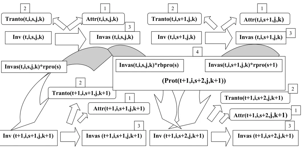
The attrition process can be seen in Figures 3.1 and 3.2 as the regions labelled 1.
3.4.2 Transition constraints (For Phase 1)
For all t,i,s,j,k,n
Trano(t,i,s,j,k,n) = Inv(t,i,s,j,k)*rtrano(i,s,n) Transition-out from branch i (combat arm), to branch n (non-combat arm) , during year t is equal to the inventory at the beginning of year t times rate of transitions out from branch i (combat arm), to branch n (non-combat arm).
For all t,i,s,j,k Tranto(t,i,s,j,k) =
∑
n
Trano(t,i,s,j,k,n)
Total transition-out from branch i (combat arm) is equal to sum of the transitions out over n , from branch i (combat arm).
The total transition-out process for combat arms (phase 1) can be seen in Figure 3.1 as the regions labelled 2.
3.4.3 Inventory constraints after attritions and transitions
(For Phase 1)For all t,i,s,j,k
Invas(t,i,s,j,k) = Inv Attr (t,i,s,j,k)-Tranto(t,i,s,j,k)
The inventory at the end of year t is equal to the inventory at the beginning of year t, minus the attritions during year t minus total transitions out from branch i (combat arm), during year t.
This process can be seen in Figure 3.1 as the regions labelled 3. (For Phase 2)
For all t,i,s,j,k
Invas(t,i,s,j,k) = Inv (t,i,s,j,k)- Attr (t,i,s,j,k)+ Tranti(t,i,s,j,k)
The inventory at the end of year t is equal to the inventory at the beginning of year t , minus the attritions during year t plus total transitions into branch i (non-combat arm), during year t .In phase 2, total transitions into branch i (non-combat arm) is parameter that is found from the arrangement of transition out variables in phase 1, according to non-combat arms. This parameter can be seen in Figure 3.2 as the regions labelled 2. This inventory process can be seen in Figure 3.2 as the regions labelled 3.
3.4.4 Promotion constraints
As mentioned before, the officers from sources NCO (Type 2) and contract officers can not promote beyond the rank of a captain (category cohort 15), therefore we branched the promotion constraints according to sources. In some special ranks, there
may be early promotions from the category cohort which is prior to the last. These are 8th category cohort for First Lieutenant, 14th category cohort for Captain, 19th category cohort for Major. Also, observe that the officers who promote early can skip only one category cohort.
For all t,i,s and j=1,2,4,5
Prot (t+1,i,s,j,k+1) = Invas (t,i,s-1,j,k)*rpro (s-1) + Invas (t,i,s-2,j,k)* rbpro (s-2)
The promotions to category cohort s, at the beginning of year t+1, for sources, Military academy(j=1), NCOs (Type 1) (j=2), CROs (j=4), Civilian (j=5), with years of service k+1 is equal to the number of promoted officers from one category cohort below plus the number of early-promoted officers from two category cohorts below.
For all t,i, 1 < s ≤ 15 and j= 3,6 Prot (t+1,i,s,j,k+1) = Invas (t,i,s-1,j,k)
The promotions to category cohort s greater than 1 and less than or equal to 15, at the beginning of year t+1, for sources NCOs (Type2) (j=3) and COs (j=6), with years of service k+1 is equal to the inventory after attritions and transitions at the end of year t, in one category cohort below. Because the officers from sources NCOs (Type 2) and COs can not benefit from early promotions and all officers in one category cohort below promote to the next category cohort, since the promotion rate is one.
For all t,i, s > 15 and j=3,6 Prot (t+1,i,s,j,k) = 0
Remember that the officers from sources, NCOs (Type 2) (j=3), COs (j=6) can not promote beyond the rank of a captain (category cohort 15). Hence the promotion to higher category cohorts than 15, for sources NCOs (Type2) and COs is zero.
The promotions to any category cohort with year of service 1 is zero. Because an officer with year of service1 is just in category cohort 1 and no promotion is available to category cohort 1.
The promotion process with general features can be seen in Figures 3.1 and 3.2 as the regions labelled 4.
3.4.5 Non-promotion constraints
Again, because of the different source characteristics, the non-promotion constraints are branched.
For all t,i,j,k, s =15
Invas(t,i,s,j,k) , if j=3,6
Notprof(t+1,i,s,j,k+1) =
0 , if j=1,2,4,5 The non-promotion from category cohort 15 , at the beginning of year t+1 with years of service k+1 is equal to the inventory after attritions and transitions, at the end of year t, since the officers from sources NCOs (Type 2) (j=3), COs (j=6) can not promote beyond the rank of a captain (category cohort 15).
For all t,i,j,k, s ≠ 15 Notprof(t+1,i,s,j,k) = 0
The non-promotions from other category cohorts should all be zero, since the total promotion rate (early promotion rate + normal promotion rate), from other category cohorts is 1.
For all t,i,s,j k=1 Notprof (t+1,i,s,j,k) = 0
3.4.6 Accession constraints
For all t,i, j=1,4,5,6 and k ≠ 1 Acc(t,i,j,k) = 0
The accession to the army, at the end of year t, from sources, Military academy (j=1), CROs (j=4), Civilian (j=5), COs (j=6), is only valid with years of service 1. Hence for other values of k, it is zero.
For all t,i, j=2 and k ≠ 7,8,9,10,11,12 Acc(t,i,j,k) = 0
The accession to the army, at the end of year t, from source NCOs (Type 1) (j=2), is only valid with years of service 7,8,9,10,11,12. Hence for other values of k, it is zero.
For all t,i, j=3 and k ≠ 7,8,9 Acc(t,i,j,k) = 0
The accession to the army, at the end of year t, from source NCOs (Type 1) (j=3), is only valid with years of service 7,8,9. Hence for other values of k, it is zero.
For all t,i,j Tacc(t,i,j) =
∑
k
Acc(t,i,j,k)
The total accession to the army from source j to branch i, at the end of year t is the sum of accessions over all k.
The accession and total accession variables are integer, hence we express the constraints in such a way that the constraints assign these variables to closest integer values.
For all t,i, j=2 and k=7,12 Acc(t,i,j,k) ≥ 0.1*Tacc(t,i,j)-1 Acc(t,i,j,k) ≤ 0.1*Tacc(t,i,j)+1
The accession to the army, from source NCOs (Type 1) (j=2), with years of service 7,12 is equal to % 10 of total accession from the same source.
For all t,i, j=2 and k=8,9,10,11 Acc(t,i,j,k) ≥ 0.2*Tacc(t,i,j)-1 Acc(t,i,j,k) ≤ 0.2*Tacc(t,i,j)+1
The accession to the army, from source NCOs (Type 1) (j=2), with years of service 8,9,10,11 is equal to % 20 of total accession from the same source.
For all t,i, j=3 and k=7 Acc(t,i,j,k) ≥ 0.4*Tacc(t,i,j)-1
Acc(t,i,j,k) ≤ 0.4*Tacc(t,i,j)+1
The accession to the army, from source NCO (Type 2) (j=3), with years of service 7 is equal to % 40 of total accession from the same source.
For all t,i, j=3 and k=8,9 Acc(t,i,j,k) ≥ 0.3*Tacc(t,i,j)-1 Acc(t,i,j,k) ≤ 0.3*Tacc(t,i,j)+1
The accession to the army, from source NCO (Type 2) (j=3), with years of service 8, 9 is equal to % 30 of total accession from the same source.
3.4.7 Capacity constraints
For all t,j
∑
k
Acc(t,i,j,k)) ≤ capu(i,j)
The total accessions from source j, at the end of year t, to branch i is less than or equal to the upper capacity of source j, marked for branch i.
For all t,i,j
∑
k
Acc(t,i,j,k)) ≥ capl(i,j)
The total accessions from source j, at the end of year t, to branch i is greater than or equal to the lower capacity of source j, marked for branch i .
3.4.8 Inventory constraints
An officer from any source starts to work in the army in the first category cohort. That means the accession to the army is only possible by the accession to the first category cohort.
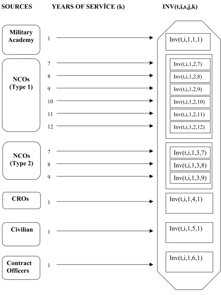
The accession process according to sources and years of service that summarizes the following three constraints can be seen in the Figure 3.3.
For all t,i,k, s=1 and j= 1,4,5,6
Acc(t,i,j,k) , if k =1 Inv(t+1,i,s,j,k)=
0 , otherwise
The accession from sources, Military academy (j=1), CROs (j=4), Civilian(j=5) and COs (j=6) is only possible with years of service 1. The inventory in category cohort 1, at the beginning of year t+1, is equal to the accessions at the end of year t, with years of
For all t,i,k, s = 1 and j = 2
Acc(t,i,j,k), if k=7,8,9,10,11,12 Inv(t+1,i,s,j,k) =
0 , otherwise
The accession from source NCOs (Type 1) (j=2) is only possible with years of service 7,8,9,10,11,12. The inventory in category cohort 1, at the beginning of year t+1 , with years of service k is equal to the accessions at the end of year t, with years of service 7,8,9,10,11,12. Since no accession is possible from this source, for other years of service values, the inventory in category cohort 1 for other years of service values, is zero.
For all t,i,k, s=1 and j=3
Acc(t,i,j,k) , if k=7,8,9 Inv(t+1,i,s,j,k) =
0 , otherwise
The accession from source NCOs (Type 2) (j=3) is only possible with years of service 7,8,9. The inventory in category cohort 1, at the beginning of year t+1 , with years of service k is equal to the accessions at the end of year t, with years of service 7,8,9. Since no accession is possible from this source, for other years of service values, the inventory in category cohort 1, for other years of service values is zero.
For all t, i, j, s > 1 and k=1 Inv(t+1,i,s,j,k) = 0
In any category cohort greater than 1, there cannot be any officers with years of service 1, hence under these conditions the inventory is zero.
The station ceilings in the ranks that are mentioned in Chapter 2 are used in the following inventory constraints to implement involuntary retirement process in the ranks.
For all t,i,j,k, 1 < s ≤ 3
Prot(t,i,s,j,k)+Notprof(t,i,s,j,k),if k ≤ 19 Inv (t,i,s,j,k)=
0 , otherwise
The inventory at the beginning of year t, in category cohort s greater than 1 and less than or equal to 3 (equivalent to rank Second Lieutenant), is equal to the promotions to category cohort s, plus the non-promotions from category cohort s.
The officers in Second Lieutenant rank with years of service greater than 19, are retired automatically since the station ceiling in this rank is 19 years of service. Hence the inventory whose years of service is greater than 19, at the beginning of year t is zero.
For all t,i,j,k, 3 < s ≤ 9 ;
Prot(t,i,s,j,k)+Notprof(t,i,s,j,k),if k ≤ 21 Inv (t,i,s,j,k) =
0 , if k > 21
Following a similar logic, the inventory at the beginning of year t, in category cohort s greater than 3 and less than or equal to 9 (equivalent to rank First Lieutenant), is calculated with the station ceiling 21 years.
For all t,i,j,k, 9 < s ≤ 15 ;
Following a similar logic, the inventory at the beginning of year t, in category cohort s greater than 9 and less than or equal to 15 (equivalent to rank Captain), is calculated with the station ceiling 21 years.
For all t,i,j,k, 15 < s ≤ 20 ;
Prot(t,i,s,j,k)+Notprof(t,i,s,j,k),if k≤ 25
Inv (t,i,s,j,k)=
0 , if k > 25 Following a similar logic, the inventory at the beginning of year t, in category cohort s greater than 15 and less than or equal to 20 (equivalent to rank Major), is calculated with the station ceiling 25 years.
For all t,i,j,k, 20 < s ≤ 23 ;
Prot(t,i,s,j,k)+Notprof(t,i,s,j,k) ,if k ≤ 27 Inv (t,i,s,j,k)=
0 , if k > 27
Following a similar logic, the inventory at the beginning of year t, in category cohort s greater than 20 and less than or equal to 23 (equivalent to rank Lieutenant Colonel), is calculated with the station ceiling 27 years.
For all t,i,j,k, 23 < s ≤ 28 ;
Prot(t,i,s,j,k)+Notprof(t,i,s,j,k), if k ≤ 31 Inv(t,i,s,j,k)=
0 , if k > 31
Following a similar logic, the inventory at the beginning of year t, in category cohort s greater than 23 and less than or equal to 28 (equivalent to rank Colonel), is calculated with the station ceiling 31 years.
For all t,i,k and s > 15 and j=3,6 Inv(t+1,i,s,j,k) =e= 0
The officers from sources NCOs (Type 2) (j=3) and CO (j=6) can not promote beyond at a rank of a captain( category cohort 15). The inventory at the beginning of year t+1 , in category cohort s greater than 15, is zero.
For all t, i, s Invtot(t,i,s) =
∑∑
j k
Inv (t,i,s,j,k)
For simplicity in further calculations , we calculated the total inventory at the beginning of year t for a specific branch and category cohort, which is equal to sum of individual inventories over all sources and years of services.
3.4.9 Rank constraints
As mentioned before, in the model, the ranks are divided into 28 category cohorts according to their current periods. Now we adjust the category cohorts to see the variables by ranks.
For all t,i, r = 1 Rinv(t,i,r) =
∑
3
1
Invtot(t,i,s)
The total inventory of Second Lieutenant rank is equal to the sum of total inventory over s less than or equal 3.
For all t,i, r = 2 Rinv(t,i,r) =
∑
9
4
For all t,i, r = 3 Rinv(t,i,r) =
∑
15
10
Invtot (t,i,s)
The total inventory of Captain rank is equal to the sum of total inventory over s greater than 9 and less than or equal to 15.
For all t,i, r = 4 Rinv(t,i,r) =
∑
2016
Invtot(t,i,s)
The total inventory of Major rank is equal to the sum of total inventory over s greater than 15 and less than or equal to 20.
For all t,i, r = 5 Rinv(t,i,r) =
∑
2321
Invtot(t,i,s)
The total inventory of Lieutenant Colonel rank is equal to the sum of total inventory over s greater than 20 and less than or equal to 23.
For all t,i, r = 6 Rinv(t,i,r) =
∑
2824
Invtot(t,i,s)
The total inventory of Colonel rank, in year t, for branch i is equal to the sum of total inventory over s greater than 23 and less than or equal to 28.
3.4.10 Balance constraints
The model can determine a solution with highly-varied accessions from the sources. However, the personnel policy does not permit big changes on number of accessions through years, especially from the source military academy. Hence we express the balance constraints to prevent high deviations among accessions from the military academy.
For all t,i, j=1
The total accessions at the end of year t+1, for source Military academy (j=1), is less than or equal the total accessions at the end of year t plus balance factor of branch i.
For all t,i,j=1
Tacc(t+1,i,j) ≥ Tacc(t,i,j)- Bf(i)
The total accessions at the end of year t+1, from source Military academy(j=1), is less than or equal the total accessions at the end of year t minus balance factor of branch i.
3.4.11
Deviation constraints
For all t,i,r
d(i,r) = Rinv(t,i,r)+ gn(t,i,r)- gp(t,i,r)
The authorized strength goal is equal to the total rank inventory in year t , plus the amount under the authorized strength goal in year t, minus the amount over the authorized strength goal in year t.
3.4.12 Objective Function
Z =
∑ ∑
∑
r t i r i t Gn r i wn(, )* ( , , )+
∑ ∑
∑
r t i r i t Gp r i wp( , )* ( , , )The objective function is to minimize the weighted sums of the values of all the negative and positive deviation variables (shortage and surplus).
3.5 Experimentation
In phase 1, we consider seven combat arms. In order to see the result for each branch in detail, we run the model for each branch one by one. This does not affect the model’s accuracy and generality, since there is no interaction among combat arms and the upper and lower capacity of sources are determined according to each branch separately. In average, for each run, there are 1261 constraints and 1455 variables and the CPU time to solve the model is 124.5 seconds. Because of the personnel policy, we do not wish to supply officers in combat arms from sources CROs, Civilian, COs. To hold this, we assign the upper capacity of these sources(capu(i,j)) to zero for all combat arms. For each branch, we assign a lower capacity for source military academy, since every year, a fixed number of officers for each branch should graduate from military academy without paying attention to the authorized strength goals. At the end of each run, we take the values of transition-out variables from combat arms to non-combat arms and after arrangement, feed them in phase 2 as transition-in parameters for non-combat arms.
In phase 2, we run the model for five non-combat arms one by one. In average, for each run, there are 1763 constraints and 1975 variables and the CPU time to solve the model is 152.1 seconds. Because of the logic as in phase 1, this does not cause any loss from the model’s accuracy and generality. However, at the beginning of each run, we enter the values of transition-in parameters. As opposed to combat arms, the non-combat arms can be provided from all sources based on the demand. As done for phase 1, the lower capacity values of each branch for source military academy are assigned.
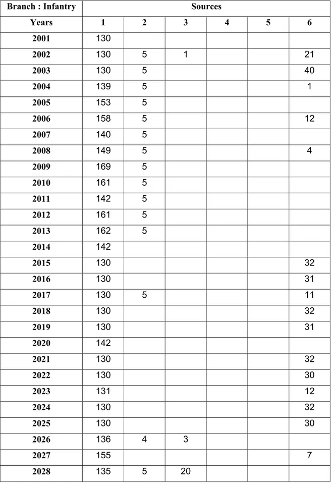
The results of the model can be seen in Appendices. Appendix A shows the accessions at the end of each year for each branch according to sources. Appendix B shows the percentage deviations from the authorized strength goal at the beginning of each year. The bold characters represent the positive deviations, others represent the negative deviations. The accessions that are determined by the model do not affect all the ranks immediately, since they enter the model from the first category cohort of first rank (Second Lieutenant). Hence, it requires some time to see the affect of the accessions on the ranks. Table 3.5 shows the minimum required time from initial year (2001) to reach the first category cohort of each rank with normal promotion.
Ranks Minimum required time Second Lieutenant 1 year (2002) First Lieutenant 4 years (2005)
Captain 10 years (2011)
Major 16 years (2017)
Lieutenant Colonel 21 years (2022)
Colonel 24 years (2025)
Table 3.5 : Minimum required time to reach ranks
After the accessions reach the first category cohort of a rank, the deviations in the rank for each branch are represented in shaded form in Appendix B, in order to see the affect of the accessions to the model.
There are high deviations for branches, Air Defense and Army Aviation (Tables B.4 and B.5) in their last ranks. This is because the huge differences between the authorized strength goal of the last rank and the authorized strength goals of previous ranks.
3.6 Scenario Analysis
As we mentioned before, the period of ranks are determined by the army. On the other hand, there are some projects about reorganizing the period of ranks to achieve the authorized strength goal and to benefit from the young officers on the battle field. After observing the negative and positive deviations in the ranks for the initial inventory and analyzing the differences among the authorized strength goals of the ranks with military manpower analysts, we proposed another alternative policy which determines to reduce the period of some ranks in which the positive deviation exists and to increase the
There may be some better alternative policy for the periods of ranks, however, because of the other social, economical and bureaucratic reasons, it may not have any chance to be implemented. The alternative policy is determined after taking into consideration these factors. One of them is the period of the junior officer(Second Lieutenant, First Lieutenant, Captain) and senior officer(Major, Lieutenant Colonel, Colonel) ranks. In the original scenario, the period of junior officer ranks is 15 years and the period of senior officer ranks is 13 years. Observe that they remain the same in the alternative scenario.
Here are the alternative periods of ranks.
Table 3.6 : The alternative periods of ranks
To see the affect of the alternative policy, first, we run the model under the original constraints and then under new constraints and finally, make a comparison between these two policies.
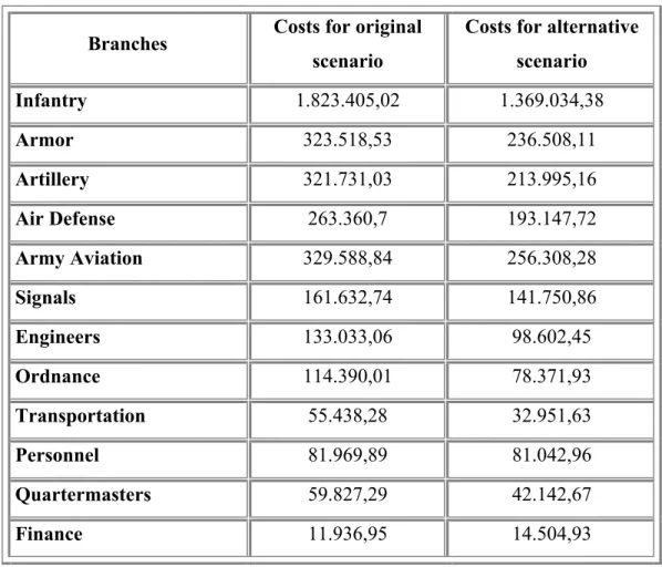
The cost of deviations for the original and alternative scenarios for each branch can be seen in Table 3.7.
RANKS ALT. PERIOD OF RANKS
Second Lieutenant 2 Years (3 years in original) First Lieutenant 7 Years (6years in original) Captain 6 Years (6 years in original) Major 6 Years (5 years in original) Lieutenant Colonel 3 Years (3 years in original) Colonel 4 Years (5 years in original)