Rotational surfaces generated by cubic hermitian and cubic bezier curves

(1)

POLİTEKNİK DERGİSİ

JOURNAL of POLYTECHNIC

ISSN: 1302-0900 (PRINT), ISSN: 2147-9429 (ONLINE) URL: http://dergipark.gov.tr/politeknik

Rotational surfaces generated by cubic

hermitian and cubic bezier curves

Kübik hermityen ve kübik bezier eğrileri

tarafından oluşturulan dönel yüzeyler

Yazar(lar) (Author(s)): Hakan GÜNDÜZ

1

_{, Ahmet KAZAN}

2

_{, H. Bayram KARADAĞ}

3

ORCID

1

_{: 0000-0003-0645-5658}

ORCID

2

_{: 0000-0002-1959-6102}

ORCID

3

_{: 0000-0001-6474-877X}

Bu makaleye şu şekilde atıfta bulunabilirsiniz(To cite to this article): Gündüz H., Kazan A. and Karadağ

H. B., “Rotational surfaces generated by cubic Hermitian and cubic bezier curves”, Politeknik Dergisi,

22(4): 1075-1082, (2019).

Erişim linki (To link to this article): http://dergipark.gov.tr/politeknik/archive

(2)

Kübik Hermityen ve Kübik Bezier Eğrileri Tarafından

Oluşturulan Dönel Yüzeyler

Araştırma Makalesi / Research Article

Hakan GÜNDÜZ1*_{, Ahmet KAZAN}2_{, H. Bayram KARADAĞ}3

1_{Faculty of Art and Science, Department of Mathematics, Inonu University, Turkey}

2_{Doğanşehir Vahap Küçük Vocational School of Higher Education, Department of Computer Technologies, Malatya Turgut Özal}

University, Turkey

3_{Faculty of Art and Science, Department of Mathematics, Inonu University, Turkey}

(Geliş/Received : 21.03.2019 ; Kabul/Accepted : 05.04.2019) ÖZ

Dönel yüzeylerin şekillerinin ayarlanmasında geometrik tasarımın istenilen şekilde olması için, ilk olarak iki yerel şekil parametreli kübik Hermityan ve kübik Bezier eğrileri kullanılarak dönel yüzeyler oluşturuldu. Oluşturulan bu yeni dönel yüzeylerin, yerel şekil parametrelerinin değiştirilmesi ile yüzeylerin şekillerinin ayarlanması konusunda iyi bir performansa sahip olduğu görüldü. Ayrıca, kübik Hermityan ve kübik Bezier eğrileri tarafından oluşturulan dönel yüzeyler, ilgi çekici yüzeylerin tasarımı için değerli bir yol sağlamaktadır. Bu bağlamda, bu dönel yüzeylerin ortalama ve Gauss eğrilikleri elde edilerek, bu yüzeyler için bazı karakterizasyonlar verildi.

Anahtar Kelimeler: Hermityen eğrileri, bezier eğrileri, dönel yüzeyler, şekil parametresi.

Rotational Surfaces Generated by Cubic Hermitian and

Cubic Bezier Curves

ABSTRACT

To tackle the geometric design in adjusting shapes of rotation surfaces, firstly the rotation surfaces have been constructed by using cubic Hermitian and cubic Bezier curves with two local shape parameters. It has been seen that, the new rotational surfaces which have been constructed have a good performance on adjusting their shapes by changing the local shape parameters. Also, the rotational surfaces generated by cubic Hermitian and cubic Bezier curves have provided a valuable way for the design of interesting surfaces. In this context, some characterizations have been given for these rotational surfaces obtaining the mean and Gaussian curvatures of them.

Keywords: Hermitian curves, bezier curves, rotational surfaces, shape parameter.

1. INTRODUCTION

Geometry of curves plays an important role in industrial design and engineering as well as being an important branch of mathematics. In recent years, many authors such as G. Farin, J. Hoschek and A. Saxena have worked on the structure of curves for mathematical modelling [5,6,10]. The most important of these curves are the Hermitian curves, Ferguson curves, Bezier curves and etc. The De Casteljau algorithm has shown that, Bezier curves are written as linear combinations of Bernstein polynomials (for detail about these curves, see [6,9,10]). Also, the geometry of surfaces such as, rotational surfaces, ruled surfaces, rational Bezier surfaces, rational B-spline surfaces, non-uniform rational B-spline surfaces, discrete surfaces and etc. have been studied by geometers and engineers widely in Euclidean space, Minkowski space, Galilean space, pseudo-Galilean space and etc [1,2,3,4,5,7,8].

For example, E. Octafiatiningsih and I. Sujarwo have used Quadratic Bezier curve on rotational and

symmetrical lampshade in [9]. So, by using this work we have constructed the present paper which is divided into three steps as follows:

i. Recalling cubic Hermitian and cubic Bezier curves; ii. rotating cubic Hermitian curve and cubic Bezier

curve about an axis to produce geometric surface designs;

iii. giving some characterizations for these rotational

surfaces obtaining the mean and Gaussian curvatures of them.

Consequently, the aim of this study is modelling some industrial objects by constructing and rotating cubic Hermitian and cubic Bezier curves and also giving new ideas for producers about object modelling industry.

2. PRELIMINARIES

A cubic Hermitian curve is a cubic polinomial curve segment constrained to a given position 𝑝 and a tangent vector 𝑣 at each endpoints.

*Sorumlu Yazar (Corresponding Author) e-posta : gunduz.haqan@hotmail.com

(3)

Hakan GÜNDÜZ, Ahmet KAZAN, H. Bayram KARADAĞ / POLİTEKNİK DERGİSİ, Politeknik Dergisi,2019;22(4): 1075-1082

Figure 1. Cubic Hermitian curve created with two control

points and two tangent segments

First, we’ll recall the parametric expression of a cubic Hermitian curve [6,10].

A parametric cubic curve 𝑃(𝑢) in Euclidean 3-space is deﬁned as P(u) = (x(u), y(u), z(u)), where

𝑥(𝑢) = 𝑎𝑥+ 𝑏𝑥𝑢 + 𝑐𝑥𝑢2+ 𝑑𝑥𝑢3,

𝑦(𝑢) = 𝑎𝑦+ 𝑏𝑦𝑢 + 𝑐𝑦𝑢2+ 𝑑𝑦𝑢3, (1)

𝑧(𝑢) = 𝑎𝑧+ 𝑏𝑧𝑢 + 𝑐𝑧𝑢2+ 𝑑𝑧𝑢3,

with parameters bounded in intervals 0 ≤ 𝑢 ≤ 1. Then, we can write it as

𝑃(𝑢) = (𝑥(𝑢), 𝑦(𝑢), 𝑧(𝑢)) = 𝑎 + 𝑏𝑢 + 𝑐𝑢2_{+ 𝑑𝑢}3_{. (2)}

Then, for 𝑢 = 0 and 𝑢 = 1, we have 𝑃(𝑢 = 0) = 𝑎,

𝑃(𝑢 = 1) = 𝑎 + 𝑏 + 𝑐 + 𝑑, (3) 𝑃′_{(𝑢 = 0) = 𝑏,}

𝑃′_{(𝑢 = 1) = 𝑏 + 2𝑐 + 3𝑑}

with 𝑎𝑥, 𝑏𝑥, 𝑐𝑥 and 𝑑𝑥 are algebraic scalar coeﬃcients.

Figure 2. Control points and tangent segments of cubic

Hermitian curve for u = 0 and u = 1

If the system (3) is solved, then the values of the vectors

a, b, c and d are obtained by

𝑎 = 𝑃(0),

𝑏 = 𝑃′(0), (4) 𝑐 = −3𝑃(0) + 3𝑃(1) − 2𝑃′(0) − 𝑃′(1),

𝑑 = 2𝑃(0) − 2𝑃(1) + 𝑃′(0) + 𝑃 ′(1).

If we use the equations (4) in (2), then the Hermitian curve is obtained as:

𝑃(𝑢) = 𝑃(0)𝐻1(𝑢) + 𝑃(1)𝐻2(𝑢) + 𝑃′(0)𝐻3(𝑢) + 𝑃′(1)𝐻4(𝑢), (5)

where 𝐻1(𝑢), 𝐻2(𝑢), 𝐻3(𝑢) and 𝐻4(𝑢) are the base

functions (or blending functions) of Hermitian curve given by

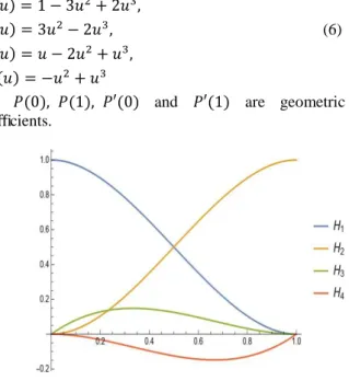
𝐻1(𝑢) = 1 − 3𝑢2+ 2𝑢3,

𝐻2(𝑢) = 3𝑢2− 2𝑢3, (6)

𝐻3(𝑢) = 𝑢 − 2𝑢2+ 𝑢3,

𝐻4(𝑢) = −𝑢2+ 𝑢3

and 𝑃(0), 𝑃(1), 𝑃′(0) and 𝑃′(1) are geometric coeﬃcients.

Figure 3. Hermitian blending functions

For the blending functions of Hermitian curve we have the following: At 𝑢 = 0 and 𝑢 = 1, we get 𝐻1= 1, 𝐻2= 𝐻3= 𝐻4= 0; 𝑃(0) = 𝑃0, 𝐻1′= 𝐻2′ = 𝐻4′ = 0, 𝐻3′ = 1; 𝑃′(0) = 𝑇0, and 𝐻1= 𝐻3= 𝐻4= 0, 𝐻2= 1; 𝑃(1) = 𝑃1, 𝐻1′= 𝐻2′ = 𝐻3′ = 0, 𝐻4′ = 1; 𝑃′(1) = 𝑇1,

respectively. This gives us the endpoints and tangent vectors at endpoints by using blending functions. Also, by putting the blending functions we can give the matrix form of cubic Hermitian curves as follows: 𝐻 = [𝐻1(𝑢), 𝐻2(𝑢), 𝐻3(𝑢), 𝐻4(𝑢)] = [𝑢3_𝑢2_{𝑢 1] [} 2 −3 0 1 −2 3 0 0 1 −2 1 0 1 −1 0 0 ] = 𝑈𝑀𝐻, (7)

where 𝑀𝐻 is called the Hermitian characteristic matrix.

Collecting the Hermitian geometric coeﬃcients into a geometric vector 𝐵, we have a matrix formulation for the Hermitian curve 𝑃(𝑢) as 𝑃(𝑢) = 𝑈𝑀𝐻𝐵, (8) where 𝐵 = [ 𝑃(0) 𝑃(1) 𝑃′(0) 𝑃′(1) ] .

𝑀𝐻 transforms geometric coordinates from the Hermitian

(4)

Next, let us recall some notations about the cubic Bezier curve [6,10].

𝑛-th degree of Bezier curve is deﬁned as (n+1) control points’ weighted linear combination using Bernstein polynomials. A Bezier curve can be expressed by

𝑃(𝑢) = ∑𝑛𝑖=0𝐶𝑖𝑛(1 − 𝑢)𝑛−𝑖𝑢𝑖𝑃𝑖 = ∑𝑛𝑖=0𝐵𝑖𝑛(𝑢)𝑃𝑖, 0 ≤ 𝑢 ≤ 1,

where 𝐵_𝑖𝑛(𝑢) is called Bernstein polynomials. More speciﬁcally, we can examine the behavior of Bezier curve for 3rd degree polynomials as follows:

Let 𝑃(𝑢) be the cubic Bezier curve lying on 𝑥𝑧-plane. It has 4 control points 𝑃_𝑖 (𝑖 = 0, 1, 2, 3) and four base functions 𝑓𝑖(𝑢) (𝑖 = 0, 1, 2, 3) with parameters bounded

in intervals 0 ≤ u ≤ 1. Then we can write it as

𝑃(𝑢) = ∑ 𝑓𝑖(𝑢)𝑃𝑖= 𝑓0(𝑢)𝑃0+ 𝑓1(𝑢)𝑃1 3

𝑖=0

+𝑓2(𝑢)𝑃2+𝑓3(𝑢)𝑃3

with the base functions 𝑓0(𝑢) = 1 − 3𝑢 + 3𝑢2− 𝑢3,

𝑓1(𝑢) = 3𝑢 − 6𝑢2+ 3𝑢3, (9)

𝑓2(𝑢) = 3𝑢2− 3𝑢3,

𝑓3(𝑢) = 𝑢3.

Figure 4. Cubic Bezier Base Functions

Also, according to the base functions, we can give the matrix form of cubic Bezier curve as follows:

𝐵 = [𝑓1(𝑢), 𝑓2(𝑢), 𝑓3(𝑢), 𝑓4(𝑢)] = [𝑢3_𝑢2_{𝑢 1] [} −1 3 −3 1 3 −6 3 0 −3 3 0 0 1 0 0 0 ] = 𝑈𝑀𝐵, (10)

where 𝑀𝐵 is called the Bezier matrix.

Collecting the Bezier geometric coeﬃcients into a geometric vector 𝐺 which is deﬁned by the user, is an array of data points. Here, we have a matrix formulation for the Bezier curve 𝑃(𝑢) as

𝑃(𝑢) = 𝑈𝑀𝐵𝐺, (11) where 𝐺 = [ 𝑃0 𝑃1 𝑃2 𝑃3 ] .

Note that the curve does not pass through the points 𝑃1 and 𝑃2. In cubic Bezier segments, in order to change

the curve’s shape we may relocate any of control points 𝑃0, 𝑃1, 𝑃2 or 𝑃3. We also know that, for Hermitian

segments, we have to specify end slopes for a particular shape and this situation is diﬃcult for researchers. Furthermore, Bezier curve is easier to specify the shape of control polyline than Hermitian curve.

For more details about Hermitian and Bezier curves, we refer to [6,9,10].

Now, let us investigate the rotational surfaces according to the axes of rotation in 𝐸3_.

Rotation is the change of an object coordinates into the new position by moving the whole coordinate points deﬁned in the initial form with an angle about an axis of rotation. The coordinate system 𝐸3 has three rotation

axes. First suppose that the axis of rotation is the 𝑧-axis. Let 𝐴 be a 3 × 3 regular matrix and 0 ≠ 𝜉 ∈ 𝐸3_{be a}

vector. If 𝐴 satisﬁes the following conditions, then it is said that 𝐴 denotes a rotation in positive direction

i. 𝐴𝜉 = 𝜉, ii. 𝐴𝐼𝐴𝑡= 𝐼, iii. det 𝐴 = 1,

where 𝐼 is the 3 × 3 unit matrix.

From this definition, it can be seen that the rotation matrix which fixes the 𝑧-axis is the set of 3 × 3 matrices defined by

𝐴(𝑣) = [cos 𝑣 − sin 𝑣 0sin 𝑣 cos 𝑣 0

0 0 1] , 𝑣 ∈ ℝ Then, by rotating the curve

𝛼(𝑢) = (𝛼1(𝑢), 𝛼2(𝑢), 𝛼3(𝑢)) about the 𝑧-axis, the

rotational surface 𝑀 can be parametrized by

Ψ(𝑢, 𝑣) = (𝛼1(𝑢) cos 𝑣 − 𝛼2(𝑢) sin 𝑣 , 𝛼1(𝑢) sin 𝑣

+𝛼2(𝑢) cos 𝑣, 𝛼3(𝑢)). (12)

By rotating the curve 𝛼 about the 𝑥-axis and 𝑦-axis, one can write the rotational surfaces similarly.

3. CONSTRUCTION OF ROTATIONAL SURFACES GENERATED BY CUBIC HERMITIAN CURVE

In this section, we’ll construct the rotational surface generated by cubic Hermitian curve by using the structure of a tube deformation.

Suppose given a tube of radius 𝑟, where 𝑟 ∈ [𝑎, 𝑏], i.e. the minimum radius of the tube is 𝑎 and the maximum of the radius is 𝑏. Also, let we deﬁne the height of the tube as ℎ, where ℎ ∈ [𝑐, 𝑑], i.e. the minimum height of the tube is 𝑐 while the maximum of the radius is 𝑑. The selection of the value of 𝑟 and ℎ in the interval aims to diﬀ erences in size of shape components of geometric design.

Firstly, we determine a center point on the tube base circle (𝑥1, 𝑦1, 𝑧1) = (0,0,0). Then, for this center point

and 𝑣 = 0 the tube base circle using the circle equation is built and the point 𝑃(0) is given by

(5)

Also, let the center point on the tube roof circle be (𝑥1, 𝑦1, 𝑧1) = (0,0, ℎ). Then, for 𝑣 = 0, we can build

tube roof circle using the circle equation and obtain the point, namely 𝑃(1) as

(𝑥1+ 𝑟2𝑐𝑜𝑠 𝑣, 𝑦1+ 𝑟2𝑠𝑖𝑛 𝑣 , 𝑧1) = (𝑟2, 0, ℎ). (14)

Then, for controlling the curvatures of the Hermitian curve, we can determine the control points 𝑃′(0) and 𝑃′(1) as follows: 𝑃′(0) = (𝑥, 0,0) (15) and 𝑃′(1) = (𝑥, 0, 𝑧), (16) where −2𝑟 ≤ 𝑥, 𝑧 ≤ 2ℎ and 𝑥, 𝑧 ∈ ℝ.

Figure 5. Representation of a tube deformation for Hermitian

curve

Further by using (13)-(16) in the equation 𝑃(𝑢) = 𝑃(0)𝐻1(𝑢) + 𝑃(1)𝐻2(𝑢) + 𝑃′(0)𝐻3(𝑢) + 𝑃′(1)𝐻4(𝑢),

the Hermitian curve is obtained by 𝑃(𝑢) = (𝑟1𝐻1(𝑢) + 𝑟2𝐻2(𝑢) + 𝑥𝐻3(𝑢) +

𝑥𝐻4(𝑢), 0, ℎ𝐻2(𝑢) + 𝑧𝐻4(𝑢)), 0 ≤ 𝑢 ≤ 1 (17)

with the blending functions (6).

3.1. Some Characterizations of Rotational Surfaces Generated By Cubic Hermitian Curve

In this subsection, ﬁrstly we’ll give some examples for rotational surface generated by cubic Hermitian curve by obtaining the parametric expression of it. Also, we’ll give some characterizations for it with the aid of the mean and Gaussian curvatures.

By rotating the Hermitian curve (17) around 𝑧-axis, we get the rotational surface as

𝑃(𝑢, 𝑣) = ([𝑟1(1 − 3𝑢2+ 2𝑢3) + 𝑟2(3𝑢2− 2𝑢3)

+ 𝑥(𝑢 − 3𝑢2_{+ 2𝑢}3_{)] cos 𝑣,}

[𝑟1(1 − 3𝑢2+ 2𝑢3) + 𝑟2(3𝑢2− 2𝑢3)

+ 𝑥(𝑢 − 3𝑢2_{+ 2𝑢}3_{)] sin 𝑣,}

ℎ(3𝑢2_{− 2𝑢}3_{) + 𝑧(−𝑢}2_{+ 𝑢}3_{)). (18)}

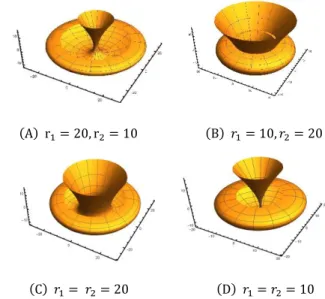
In the following ﬁgures, one can see the rotational surface (18) for 𝑥 = 100, ℎ = 15, 𝑧 = 150 and diﬀ erent radius 𝑟1 and 𝑟2:

(A) r1= 20, r2= 10 (B) 𝑟1= 10, 𝑟2= 20

(C) 𝑟1= 𝑟2= 20 (D) 𝑟1= 𝑟2= 10

Figure 6. Rotational surface (18) for diﬀ erent radius

Now, by taking 𝑟1= 𝑟2= 𝑟 in (18), we can write the

rotational surface generated by cubic Hermitian curve as

𝑃(𝑢, 𝑣) = ([𝑟 + 𝑥(𝑢 − 3𝑢2_{+ 2𝑢}3_{)] cos 𝑣,}

[𝑟 + 𝑥(𝑢 − 3𝑢2_{+ 2𝑢}3_{)] sin 𝑣,}

ℎ(3𝑢2_{− 2𝑢}3_{) + 𝑧(−𝑢}2_{+ 𝑢}3_{)). (19)}

In the following ﬁgures, one can see the Hermitian curve and rotational surface (19) generated by this cubic Hermitian curve for 𝑟 = 10, 𝑥 = 300, ℎ = 15, 𝑧 = 400:

(𝐴) Hermitian curve (𝐵) Rotational surface

Figure 7. Hermitian curve and rotational surface (19)

The coeﬃcients of the ﬁrst and second fundamental forms of the rotational surface (19) are obtained as 𝐸 = 𝑥2_{(1 − 6𝑢 + 6𝑢}2₎2 +[6ℎ𝑢(1 − 𝑢) + 𝑧𝑢(−2 + 3𝑢)]2_, 𝐹 = 0, (20) 𝐺 = [𝑟 + 𝑥(𝑢 − 3𝑢2_{+ 2𝑢}3_)]2 and 𝐿 = 2𝑥 √𝐷[3ℎ(1 − 2𝑢) − 𝑧(1 − 3𝑢 + 3𝑢 2₎_], 𝑀 = 0, (21) 𝑁 = 1 √𝐷[𝑟 + 𝑥(𝑢 − 3𝑢 2_{+ 2𝑢}3_)]_× [6ℎ𝑢(1 − 𝑢) + 𝑧𝑢(−2 + 3𝑢)],

(6)

respectively. Here, the unit normal of the surface is 𝑁(𝑢, 𝑣) = 1 √𝐷(−[6ℎ𝑢(1 − 𝑢) + 𝑧𝑢(−2 + 3𝑢)] cos 𝑣, −[6ℎ𝑢(1 − 𝑢) + 𝑧𝑢(−2 + 3𝑢)] sin 𝑣, 𝑥(1 − 6𝑢 + 6𝑢2₎₎ and 𝐷 = [6ℎ𝑢(1 − 𝑢) + 𝑧𝑢(−2 + 3𝑢)]2 +𝑥2_{(1 − 6𝑢 + 6𝑢}2₎2_.

So, we can give the following Theorem:

Theorem 1. The mean curvature and Gaussian curvature

of the rotational surface (19) are

𝐻 = 2𝑥[𝑟 + 𝑥(𝑢 − 3𝑢2_{+ 2𝑢}3_)]_× [3ℎ(1 − 2𝑢)− 𝑧(1 − 3𝑢 + 3𝑢2₎_]₊ [𝑥2₍_{1 − 6𝑢 + 6𝑢}2₎2₊_[_6ℎ𝑢₍_{1 − 𝑢}₎_{+ 𝑧𝑢}₍_{−2 + 3𝑢}_)]2_]_× [6ℎ𝑢(1 − 𝑢)+ 𝑧𝑢(−2 + 3𝑢)] 2[𝑥2₍_{1 − 6𝑢 + 6𝑢}2₎2₊_[_6ℎ𝑢₍_{1 − 𝑢}₎_{+ 𝑧𝑢}₍_{−2 + 3𝑢}_)]2_]32× [𝑟 + 𝑥(𝑢 − 3𝑢2_{+ 2𝑢}3₎] and (22) 𝐾 = 2𝑥[3ℎ(1 − 2𝑢)− 𝑧(1 − 3𝑢 + 3𝑢2₎_]_× [6ℎ𝑢(1 − 𝑢)+ 𝑧𝑢(−2 + 3𝑢)] [𝑥2₍_{1 − 6𝑢 + 6𝑢}2₎2₊_[_6ℎ𝑢₍_{1 − 𝑢}₎_{+ 𝑧𝑢}₍_{−2 + 3𝑢}_)]2_]2_× [𝑟 + 𝑥(𝑢 − 3𝑢2_{+ 2𝑢}3₎_] , (23) respectively.

The following ﬁgures show the Gaussian and mean curvatures functions’ graphics of the rotational surface (19) for 𝑟 = 10, 𝑥 = 300, ℎ = 15, 𝑧 = 400 and the variations of Gaussian and mean curvatures on this surface:

(𝐴) Gaussian curvature (𝐵) Mean curvature function’s graphic function’s graphic

(C) Variation of Gaussian (D) Variation of mean curvature curvature on surface on surface

Figure 8. Gaussian and mean curvatures’ graphics and the

variations of Gaussian and mean curvatures on surface

Now, let us take 𝑧 = 2ℎ in the equations (19)-(23). Then, we have

𝑃(𝑢, 𝑣) = ([𝑟 + 𝑥(𝑢 − 3𝑢2_{+ 2𝑢}3_{)] cos 𝑣,}

[𝑟 + 𝑥(𝑢 − 3𝑢2_{+ 2𝑢}3_{)] sin 𝑣, ℎ𝑢}2_{). (24)}

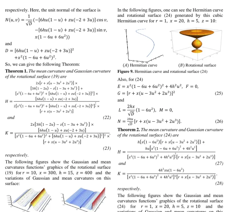
In the following ﬁgures, one can see the Hermitian curve and rotational surface (24) generated by this cubic Hermitian curve for 𝑟 = 1, 𝑥 = 20, ℎ = 5, 𝑧 = 10:

(𝐴) Hermitian curve (𝐵) Rotational surface

Figure 9. Hermitian curve and rotational surface (24)

Also, for (24) 𝐸 = 𝑥2_{(1 − 6𝑢 + 6𝑢}2₎2_{+ 4ℎ}2_𝑢2_{, 𝐹 = 0,} 𝐺 = [𝑟 + 𝑥(𝑢 − 3𝑢2_{+ 2𝑢}3_)]2 ₍₂₅₎ and 𝐿 =2ℎ𝑥 √𝐷 (1 − 6𝑢 2_{), 𝑀 = 0,} 𝑁 =2ℎ𝑢_√𝐷 [𝑟 + 𝑥(𝑢 − 3𝑢2_{+ 2𝑢}3_{)]. (26)}

𝐻 = ℎ{𝑥(1 − 6𝑢2_)[_{𝑟 + 𝑥}₍_{𝑢 − 3𝑢}2_{+ 2𝑢}3_)]}₊ ℎ𝑢[𝑥2_{(1 − 6𝑢 + 6𝑢}2₎2 + 4ℎ2_𝑢2_] [𝑥2_{(1 − 6𝑢 + 6𝑢}2₎2_{+ 4ℎ}2_𝑢2]32[𝑟 + 𝑥(𝑢 − 3𝑢2+ 2𝑢3)] and (27) 𝐾 = 4ℎ 2_{𝑥𝑢(1 − 6𝑢}2₎ [𝑥2_{(1 − 6𝑢 + 6𝑢}2₎2_{+ 4ℎ}2_𝑢2_]2_[_{𝑟 + 𝑥}₍_{𝑢 − 3𝑢}2_{+ 2𝑢}3_)] , (28) respectively.

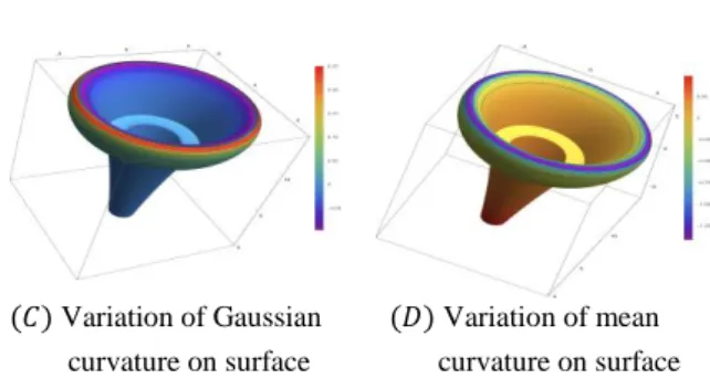
The following ﬁgures show the Gaussian and mean curvatures functions’ graphics of the rotational surface (24) for 𝑟 = 1, 𝑥 = 20, ℎ = 5, 𝑧 = 10 and the variations of Gaussian and mean curvatures on this surface:

(𝐴) Gaussian curvature’s (𝐵) Mean curvature’s

graphic graphic

(C) Variation of Gaussian (D) Variation of mean curvature on surface curvature on surface

(7)

Now, from (27) and (28) we can give the following characterizations:

Corollary 1. Let M be the rotational surface (24) which

is generated by cubic Hermitian curve.

i. Then, the mean curvature of surface cannot vanish at the initial point of the Hermite curve.

ii. Then, the mean curvature of surface vanishes at the ending point of the Hermite curve if and only if the equation 5ℎ𝑟𝑥 = 𝑥2+ 4ℎ2 holds.

iii. If the mean curvature of surface vanishes at the ending point of the Hermite curve, then the control point of 𝑃′(1) cannot be on the z-axis or the control point of 𝑃′(0) cannot be on the origin.

Corollary 2. Let M be the rotational surface (24) which

is generated by cubic Hermitian curve. Then, the Gaussian curvature of surface

i. vanishes at the initial point of the Hermite curve;

ii. vanishes on the parametric curve 𝑃(1

√6, 𝑣) of 𝑀;

iii. vanishes, if the control point of 𝑃′(1) is on the 𝑧-axis or the control point of 𝑃′(0) is on the origin.

4. CONSTRUCTION OF ROTATIONAL

SURFACES GENERATED BY CUBIC BEZIER CURVE

In this section, we’ll construct the rotational surface generated by cubic Bezier curve by using the structure of a tube deformation.

Suppose given a tube of radius 𝑟1 and 𝑟2, where

𝑟1, 𝑟2∈ [𝑎, 𝑏]. Also, let we deﬁne the height of the

tube as ℎ, where ℎ ∈ [𝑐, 𝑑]. The selection of the value of 𝑟1, 𝑟2 and ℎ in the interval aims to diﬀ erences in size

of shape components of geometric design.

Firstly, we determine a center (initial) point on the tube base circle (𝑥1, 𝑦1, 𝑧1) = (0,0,0). Then, for this center

(initial) point and 𝑣 = 0 the tube base circle using the circle equation is built and the point 𝑃0 is given by

𝑃0= (𝑥1+ 𝑟1cos 𝑣, 𝑦1+ 𝑟1sin 𝑣 , 𝑧1) = (𝑟1, 0,0). (29)

Also, let the center (ending) point on the tube roof circle be (𝑥1, 𝑦1, 𝑧1) = (0,0, ℎ). Then, for 𝑣 = 0, we can build

tube roof circle using the circle equation and obtain the point, namely 𝑃3 as

𝑃3= (𝑥1+ 𝑟2cos 𝑣, 𝑦1+ 𝑟2sin 𝑣 , 𝑧1) = (𝑟2, 0, ℎ). (30)

Then, the other two control points 𝑃1 and 𝑃2 of the cubic

Bezier curve can be deﬁned as follows:

𝑃1= (𝑥1, 0, 𝑧1) (31)

and

𝑃2= (𝑥2, 0, 𝑧2). (32)

Figure 11. Representation of a tube deformation for Bezier

curve

Further by using (29)-(32) in the equation

𝑃(𝑢) = 𝑓0(𝑢)𝑃0+ 𝑓1(𝑢)𝑃1+ 𝑓2(𝑢)𝑃2+ 𝑓3(𝑢)𝑃3,

the Bezier curve is obtained by

𝑃(𝑢) = (𝑟1𝑓0(𝑢) + 𝑥1𝑓1(𝑢) + 𝑥2𝑓2(𝑢) + 𝑟2𝑓3(𝑢), 0,

𝑧1𝑓1(𝑢) + 𝑧2𝑓2(𝑢) + ℎ𝑓3(𝑢)), 0 ≤ 𝑢 ≤ 1 (33)

with the base functions (9).

4.1. Some Characterizations of Rotational Surfaces Generated By Cubic Bezier Curve

In this subsection, ﬁrstly we’ll give some examples for rotational surface generated by cubic Bezier curve by obtaining the parametric expression of it. Also, we’ll give some characterizations for it with the aid of the mean and Gaussian curvatures.

By rotating the Bezier curve (33) around z-axis, we get the rotational surface 𝑃(𝑢, 𝑣) with two local shape parameters as ([𝑟1(1 − 3𝑢 + 3𝑢2− 𝑢3) + 𝑥1(3𝑢 − 6𝑢2+ 3𝑢3) + 𝑥2(3𝑢2− 3𝑢3) + 𝑟2𝑢3] cos 𝑣, [𝑟1(1 − 3𝑢 + 3𝑢2− 𝑢3) + 𝑥1(3𝑢 − 6𝑢2+ 3𝑢3) + 𝑥2(3𝑢2− 3𝑢3) + 𝑟2𝑢3] sin 𝑣, 𝑧1(3𝑢 − 6𝑢2+ 3𝑢3) + 𝑧2(3𝑢2− 3𝑢3) + 𝑢3ℎ). (34)

In the Figure 12, one can see the rotational surface (34) for diﬀ erent values of 𝑟1, 𝑟2, 𝑥1, 𝑥2,, 𝑧1, 𝑧2 and ℎ which

have been choosed as following, respectively:

(𝐴) 𝑟1= 2, 𝑟2= 0, 𝑥1= 5, 𝑥2= 10, 𝑧1= 10, 𝑧2= 2 and ℎ = 0.1; (𝐵) 𝑟1= 1, 𝑟2= 2, 𝑥1= 10, 𝑥2= 5, 𝑧1= 25, 𝑧2= 10 and ℎ = 1; (𝐶) 𝑟1= 1, 𝑟2= 2, 𝑥1= 20, 𝑥2= 5, 𝑧1= 20, 𝑧2= 5 and ℎ = 20; (𝐷) 𝑟1= 1, 𝑟2= 2, 𝑥1= 50, 𝑥2= 35, 𝑧1= 40, 𝑧2= 25 and ℎ = 90.

(8)

(𝐴) (𝐵)

(𝐶) (𝐷)

Figure 12. Rotational surface (34) for diﬀ erent values of

𝑟1, 𝑟2, 𝑥1, 𝑥2,, 𝑧1, 𝑧2 and ℎ

The ﬁrst derivative of the surface (34) with respect to u and v are 𝑃𝑢(𝑢, 𝑣) = ([𝑟1(−3 + 6𝑢 − 3𝑢2) + 𝑥1(3 − 12𝑢 + 9𝑢2) + 𝑥2(6𝑢 − 9𝑢2) + 3𝑢2𝑟2] 𝑐𝑜𝑠 𝑣, [𝑟1(−3 + 6𝑢 − 3𝑢2) + 𝑥1(3 − 12𝑢 + 9𝑢2) + 𝑥2(6𝑢 − 9𝑢2) + 3𝑢2𝑟2] sin 𝑣, 𝑧1(3 − 12𝑢 + 9𝑢2) + 𝑧2(6𝑢 − 9𝑢2) + 3𝑢2ℎ) 𝑃𝑣(𝑢, 𝑣) = (−𝜌 sin 𝑣, 𝜌 cos 𝑣, 0) where 𝜌 = 𝑟1(1 − 3𝑢 + 3𝑢2− 𝑢3) + 𝑥1(3𝑢 − 6𝑢2+ 3𝑢3_{) + 𝑥} 2(3𝑢2− 3𝑢3) + 𝑟2𝑢3, 0 ≤ 𝑢 ≤ 1. So the

coeﬃcients of ﬁrst fundamental form of rotational surface (34) are obtained as

𝐸 = 𝛽2_{+ 𝜃}2_, 𝐹 = 0, (35) 𝐺 = 𝜌2_, where 𝛽 = 𝑟1(−3 + 6𝑢 − 3𝑢2) + 𝑥1(3 − 12𝑢 + 9𝑢2) + 𝑥2(6𝑢 − 9𝑢2) + 3𝑢2𝑟2, 𝜃 = 𝑧1(3 − 12𝑢 + 9𝑢2) + 𝑧2(6𝑢 − 9𝑢2) + 3𝑢2ℎ.

Also, the unit normal of the surface can be found as

𝑁(𝑢, 𝑣) = 1

√𝜃2_{+ 𝛽}2(−𝜃 cos 𝑣, −𝜃 sin 𝑣 , 𝛽).

The second derivatives of 𝑃(𝑢, 𝑣) are given by 𝑃𝑢𝑢(𝑢, 𝑣) = ([𝑟1(6 − 6𝑢) + 𝑥1(−12 + 18𝑢) + 𝑥2(6 − 18𝑢) + 6𝑢𝑟2] cos 𝑣, [𝑟1(6 − 6𝑢) + 𝑥1(−12 + 18𝑢) + 𝑥2(6 − 18𝑢) + 6𝑢𝑟2] sin 𝑣, 𝑧1(−12 + 18𝑢) + 𝑧2(6 − 18𝑢) + 6𝑢ℎ), 𝑃𝑢𝑣(𝑢, 𝑣) = (−𝛽 sin 𝑣, 𝛽 cos 𝑣 , 0), 𝑃𝑣𝑣(𝑢, 𝑣) = (−𝜌 cos 𝑣, −𝜌 sin 𝑣, 0).

Then, the coeﬃcients of second fundamental form of rotational surface are obtained by

𝐿 =−𝜎𝜃 + 𝜇𝛽 √𝜃2_{+ 𝛽}2, 𝑀 = 0, (36) 𝑁 = 𝜌𝜃 √𝜃2_{+ 𝛽}2, respectively. Here, 𝜎 = 𝑟1(6 − 6𝑢) + 𝑥1(−12 + 18𝑢) + 𝑥2(6 − 18𝑢) + 6𝑢𝑟2 and 𝜇 = 𝑧1(−12 + 18𝑢) + 𝑧2(6 − 18𝑢) + 6𝑢ℎ.

We have the following theorem.

𝐻 =𝜃(𝛽2+𝜃2)+𝜌(𝜇𝛽−𝜎𝜃) 2𝜌(𝛽2_+𝜃2₎32 (37) and 𝐾 =_𝜌(𝛽𝜃(𝜇𝛽−𝜎𝜃)₂_+𝜃₂₎₂ , (38) respectively.

In the following ﬁgures, one can see the cubic Bezier curve and rotational surface (34) generated by this cubic Bezier curve for 𝑟₁= 1, 𝑟₂= 2, 𝑥₁= 5, 𝑥₂= 10, 𝑧1= 25, 𝑧2= 10, ℎ = 10:

(𝐴) Bezier curve (𝐵) Rotational surface (34)

Figure 13. Bezier curve and rotational surface (34)

The following ﬁgures show the Gaussian and mean curvatures functions’ graphics of the rotational surface (34) and the variations of Gaussian and mean curvatures on this surface:

(𝐴) Gaussian curvature (𝐵) Mean curvature function’s graphic function’s graphic

(9)

(𝐶) Variation of Gaussian (𝐷) Variation of mean curvature on surface curvature on surface

variations of Gaussian and mean curvatures on surface

Now, from (37) and (38), let us give some characterizations for rotational surface (34) generated by cubic Bezier curve.

Corollary 3. Let 𝑀 be the rotational surface (34) which

is generated by cubic Bezier curve.

i. If the control point of 𝑃1 is on the 𝑥-axis, then the

mean curvature of the surface cannot vanish at the initial point of the Bezier curve.

ii. If the control point of 𝑃1 is on the origin, then

the mean curvature of the surface cannot vanish at the initial point of the Bezier curve.

iii. If the control point of 𝑃₁ is on the 𝑥-axis, then the

Gaussian curvature of the surface vanishes at the initial point of the Bezier curve.

iv. If the control point of 𝑃2 is on the origin, then the

Gaussian curvature of the surface cannot vanish at the initial point of the Bezier curve.

v. If the control points of 𝑃₂ and 𝑃₃ are on the 𝑥-axis, then the mean curvature of the surface cannot vanish at the ending point of the Bezier curve.

vi. If the control points of 𝑃₂ and 𝑃₃ are on the

𝑥-axis, then the Gaussian curvature of the surface vanishes at the ending point of the Bezier curve.

vii. If the control point of 𝑃2 is on the origin and

the equation 𝑥₁ℎ = 𝑧₁𝑟₂, then the Gaussian curvature of the surface vanishes at the ending point of the Bezier curve.

5. CONCLUSION

In the present study, we have used Hermitian and Bezier curves in the cubic structure and applied a rotation to these curves. Based on these curves, we have obtained geometric shapes as the result of rotating surfaces. Industrial objects such as lampshades, vases, bullets, etc. provide less costly, more convenient and more reliable results through the use of these structures. In this context, by changing the values of constants 𝑟₁, 𝑟₂, 𝑥₁, 𝑥₂, 𝑧₁, 𝑧₂ and ℎ, diﬀ erent curves and rotational surfaces generated by these curves can be obtained. In the geometric sense, some characterizations which have been obtained with

the aid of mean and Gaussian curvatures of the rotational surfaces generated by these curves have been examined. The beneﬁts of this study for industrial design are: 1. With the help of computer, some new procedure for modelling some industrial objects can be obtained. 2. New ideas for producers about some object models industry in the form of geometric surface design so as to increase the choice of existing models previously can be provided.

Furthermore, by deﬁning the cubic Hermitian and cubic Bezier curves in diﬀ erent spaces, such as Lorentz-Minkowski space, Galilean space and pseudo Galilean space, these curves and rotational surfaces can be investigated as a future work.

REFERENCES

[1] Arslan K., Bulca B. and Kosova D., “On Generalized Rotational Surfaces in Euclidean Spaces”, J. Korean

Math. Soc., (2017).

[2] Baikoussis C. and Blair D.E., “On the Gauss map of ruled surfaces”, Glasgow Math. J., 34: 355-359, (1992). [3] Bobenko A. and Pinkall U., “Descrete sothermic

Surfaces”, J. reine angev, Math, 475: 187-208, (1996). [4] Chen B.Y., Choi M. and Kim Y.H, “Surfaces of

revolution with pointwise 1-type Gauss map”, J. Korean

Math. Soc., 42(3): 447-455, (2005).

[5] Dietz R., Hoschek J. and Juettler B., “An algebraic approach to curves and surfaces on the sphere and on other quadrics”, Computer Aided Geometric Design, 10: 211-229, (1993).

[6] Farin G., “Curves and Surfaces for CAGD: A Practical Guide”, Academic Press Inc, San Diego (2002). [7] Kazan A. and Karadağ H. B., “A classification of

Surfaces of Revolution in Lorentz-Minkowski Space”,

Int. J. Contemp. Math. Sciences, 6(39): 1915-1928,

(2011).

[8] Kazan A. and Karadağ H. B., “Weighted Minimal and Weighted Flat Surfaces of Revolution in Galilean 3-Space with Density’’, Int. J. of Analysis and

Applications, 16(3): 414-426, (2018).

[9] Octafiatiningsih E. and Sujarwo I., “The Application of Quadratic Bezier Curve on Rotational and Symmetrical Lampshade”, Cauchy-Journal of Pure and Applied

Mathematics, 4(2): 100-106, (2016).

[10] Saxena A. Saxena Sahay B., “Computer Aided

Engineering Design”, Anamaya Publishers, New Delhi,