Evidence of Possible Recharge Zones for Lake Salda (Turkey)

– to permeabilize the cells for optimal probe target interaction – to maintain cell morphology. • Cannot detect small mutations. • Probes are not yet commercially available for all

Electric Vehicle Routing Problem with Time Windows and Stochastic Waiting Times at Recharging Stations 5.1.. Related

So, in the case the EV is recharged only once during its route then: (i) if the customer is inserted between the depot and the station the insertion only affects the arrival state

Our aim in this study was to determine current conditions of zooplankton fauna of Abant Lake, which was studied seasonally, and could provide resources for future

Aşırı Turizm Kapsamında Salda Gölü’nün Fiziksel Taşıma Kapasitesinin Belirlenmesi (Determining the Physical Carrying Capacity of Salda Lake in the Scope of Overtourism).. *

‘Aşırı turizmin etkileri’ olarak adlandırılan bu ana tema içerisinde ziyaretçilerin Salda Gölü’ne yönelik yaptıkları değerlendirmeler “Çevre Kirliliği ve

Due to non-existence of ground lake level measurements following the lakes level falling below gage in 2004, WSE had to be calculated using LAB in which; AL/w bathymetry is used

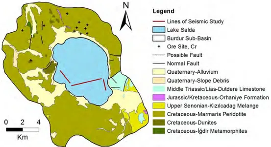
The agricultural areas and handicapped forests are potential threats for the soil erosion and river pollution particularly at the steep slopes of the river

References

Altınlı, I˙. E. (1955). The Geology of Southern Denizli. I˙stanbul University Journal of Science Faculty, 1(2), 1–45.
Baykal, B. B., Go¨nenc¸, I. E., Meric¸, M., Tanik, A., Tunay, O., et al. (1996). An alternative approach for evaluation of lake water
(12)
quality: Lake Sapanca—A case study from Turkey. Water Science and Technology, 34(12), 73–81.
Bielsa, C. P., Lamba´n, L. J., Plata, J. L., Rubio, F. M., Soto, R., et al. (2012). Characterization of a karstic aquifer using magnetic resonance sounding and electrical resistivity tomography: A case-study of Estan˜a Lakes (northern Spain). Hydrogeology Journal, 20, 1045–1059.
Bodinier, J. L., & Godard, M. (2014). Reference module in earth systems and environmental science. Treatise on Geochemistry, 3, 103–167.
Bonansea, M., Rodriquez, M. C., Pinotti, L., Ferrero, S., et al. (2015). Using multi-temporal Landsat imagery and linear mixed models for assessing water quality parameters in Rio Tercero reservoir (Argentina). Remote Sensing of Environment, 158, 28–41. Braithwaite, C. J. R., & Zedef, V. (1994). Living hydromagnesite
stromatolites from Turkey. Sedimentary Geology, 92, 1–5. Caldirak, H., Kurtulus, B., Canoglu, M. C., Tunca, E., et al. (2017).
Heavy metal contamination profiles and accumulation patterns in Lake Salda, Turkey. Fresenius Environmental Bulletin, 26(12A), 8047–8061.
Canog˘lu, M. C. (2015). An investigation on the surface water effect in landslide susceptibility mapping: An example from Yenice (Karabu¨k) basin. Ph.D. thesis, Institue of Science of Hacettepe University.
Chile`s, J.-P., & Delfiner, P. (2012). Geostatistics: Modeling spatial uncertainty (2nd ed.). Hoboken: Wiley.
Crescentini, M., Bennati, M., Tartagni, M., et al. (2012). Design of integrated and autonomous conductivity–temperature–depth (CTD) sensors. International Journal of Electronics and Com-munications, 66, 630–635.
Du, C., Ren, H., Qin, Q., Meng, J., Zhao, S., et al. (2015). A practical split-window algorithm for estimating land surface temperature from Landsat 8 data. Remote Sensing, 7, 647–665.
Ersoy, S¸. (1989). Geology of the Guney Mountain and Kelebek Mountain located between Fethiye (Mug˘la)–Go¨lhisar (Burdur) area. Ph.D. Thesis, Istanbul University Institute of Graduate Studies in Science.
ESRI. (2013). ArcGIS desktop: Release 10.2. Redlands, CA: Envi-ronmental Systems Research Institute.
Finzgar, N., Jez, E., Voglar, D., & Lestan, D. (2014). Spatial distribution of metal contamination before and after remediation in the Meza Valley, Slovenia. Geoderma, 217–218, 135–143. Kazancı, N., So¨nmez, G., Du¨gel, M., et al. (2004). On the limnology
of Salda Lake, A large and deep soda lake in southwestern
Turkey: Future management proposals. Aquatic Conservation: Marine and Freshwater Ecosystems, 14, 151–162.
Kocaefe, S., & Ataman, G. (1976). Seismotectonic events in Anatolia-1: Investigation of the area within the Antalya–Fethiye–Denizli triangle. Bulletin for Earth Sciences, 1(1), 55–70.
Krivoruchko, K. (2011). Spatial statistical data analysis for GIS users (p. 928). Redlands, CA: ESRI Press.
Markham, B. L., & Barker, J. K. (1985). Spectral characteristics of the LANDSAT Thematic Mapper sensors. International Journal of Remote Sensing, 6, 697–716.
MTA. (2010). 1/:100000 Scale Geological Maps of Turkey. Report No.: 16 Second Edition Publication of Mineral Research and Exploration Institute of Turkey.
Mu¨ller, G., Irion, G., Fo¨rstner, U., et al. (1972). Formation and diagenesis of inorganic Ca–Mg carbonates in the lacustrine environment. The Science of Nature, 59, 158–164.
Poisson, A. (1977). Geological Research in Western Taurides (Turkey). Ph.D. Thesis, Paris-Sud (Orsay) State University. Russell, M. J., Ingham, J. K., Zedef, V., Maktav, D., Sunar, F., Hall,
A. J., et al. (1999). Search for signs of ancient life on Mars: Expectations from hydromagnesite microbialites, Salda Lake, Turkey. Geological Society of London Journal, 156, 869–888. Sarp, H. (1976). Etude geoloqique et petropraphique du Cortege
Ophiolitique de la Region Situee au Nord-Ouest de Yes¸ilova (Burdur-Turkey). Thesis, University of Geneve.
Thuizat, R., Whitechurch, H., Montigny, R., & Juteau, T. (1981). K-Ar dating of some infraophiolitic metamorphic soles from the Eastern Mediterranean. New Evidence for oceanic thrusting before obduction, Earth and Planetary Science Letters, 52, 302–310.
Trescott, A., & Park, M. H. (2014). Remote sensing models using Landsat satellite data to monitor algal blooms in Lake Cham-plain. Water Science and Technology, 67, 1113–1120. Tunca, E., Ucuncu, E., Kurtulus¸, B., Ozkanc, A. D., Atasagun, S.,
et al. (2013). Accumulation effects and trends of some heavy metal (Al, Cu, Fe, Ni, Zn) and a metalloid (As) in the freshwater crayfish. Ecology and Chemistry, 29, 754–769.
Vlassova, L., Perez-Cabello, F., Nieto, H., Martı´n, P., Rian˜o, D., de la Riva, J., et al. (2014). Assessment of methods for land surface temperature retrieval from Landsat-5 TM images applicable to multiscale tree-grass ecosystem modeling. Remote Sensing, 6, 4345–4368.
Wetzel, R. G. (2001). Limnology. Lake and river ecosystems. San Diego: Elsevier Academic Press.
Şekil
Fig. 1 Studied domain: location of study area, topographic relief map, observation points and streamsLegend
Fig. 2 Geological map of the region [modified from MTA