Tarım Bilimleri Dergisi
Tar. Bil. Der.
Dergi web sayfası: www.agri.ankara.edu.tr/dergi
Journal of Agricultural Sciences
Journal homepage: www.agri.ankara.edu.tr/journal
TARIM BİLİMLERİ DERGİSİ
—
JOURNAL OF AGRICUL
TURAL SCIENCES
21 (2015) 123-131
A New Approach for Determination of Seed Distribution Area in
Vertical Plane
Sefa ALTIKATa, Alper GÜLBEb, Ahmet ÇELİKc
aIğdır University, Faculty of Agriculture, Department of the Biosystem Engineering, Iğdır, TURKEY
bIğdır University, Technical Sciences Vocational School, Department of Computer Programming, Iğdır, TURKEY c Atatürk University, Faculty of Agriculture, Department of the Agricultural Machinery, Erzurum, TURKEY
ARTICLE INFO
Research Article
Corresponding Author: Sefa ALTIKAT, E-mail: [email protected], Tel: +90 (476) 226 20 12 Received: 14 May 2014, Received in Revised Form: 22 July 2014, Accepted: 20 August 2014
ABSTRACT
The objective of this study was to develop a new method to evaluate the seed distribution area in vertical plane and compare it with the other methods. For this purpose, the different calculation methods of seed distribution area namely, standard deviational ellipse, voronoi polygons with delaunay triangulation, integral method, and developed one, the concave hull algorithm was considered and compared in this study. Three different types of no-till seeders equipped with hoe (NS1), single disc (NS2) and winged hoe (NS3) type openers were used and operated at three different tractor
forward speeds (0.75 m s-1, 1.25 m s-1 and 2.25 m s-1). According to the results obtained from the study, it was found
that the newly developed seed distribution evaluation procedure, concave hull, provided the smaller area values of the distributed seeds as compared to others. The influences of seeders were tested and it was found that the no-till seeder which has disc type furrow opener spread the seeds into larger areas. However, maximum variations of sowing depth values were observed at the no-till seeder with single disc furrow opener. Increasing tractor forward speeds resulted in an increased variation of sowing depth.
Keywords: Ellipse; Voronoi; Integral; Concave hull algorithm; No-till seeder; Tractor forward speed
Düşey Düzlemdeki Tohum Dağılım Alanının Belirlenmesinde Yeni Bir
Yaklaşım
ESER BİLGİSİ
Araştırma Makalesi
Sorumlu Yazar: Sefa ALTIKAT, E-posta: [email protected], Tel: +90 (476) 226 20 12 Geliş Tarihi: 14 Mayıs 2014, Düzeltmelerin Gelişi: 22 Temmuz 2014, Kabul: 20 Ağustos 2014
ÖZET
Bu araştırmanın amacı, tohum dağılım alanının değerlendirilmesine yeni bir yaklaşım geliştirmektir. Bu amaçla, standart sapmalı elips, delaunay üçgenlemesiyle voronoi poligonları ve integral metodu gibi farklı tohum dağılım alanı hesaplama yöntemleri karşılaştırılmış ve içbükey zarf adı verilen yeni bir yöntem geliştirilmiştir. Araştırmada, çapa (NS1),
124
Ta r ı m B i l i m l e r i D e r g i s i – J o u r n a l o f A g r i c u l t u r a l S c i e n c e s 21 (2015) 123-1311. Introduction
Seed distribution as an important factor affecting seed emergence and productivity is expressed in lateral and vertical plane during sowing process. The factors affecting uniform seed distribution in horizontal plane are the distribution of seed spacing in a row and deviations from the furrow.
The purpose of sowing is to place seeds into preferred depth and distance within the row. The coefficient of variation which is the standard deviation of the sowing depths expressed as percentage of the mean seeding depth can be used to indicate the uniformity of the seeding depth. A coefficient of variation (CV%) value under 30% represents acceptable sowing depth (ISO 1984).
Karayel & Özmerzi (2001) have stated that the seed distribution in vertical plane relevant to seed distribution area depends on the sowing depth. Besides, Wilkins et al (1991) have stated that the “Stampede” peas had yield rise with spacing uniformity but “Bolero” peas had no sensitivity on uniformity of plant spacing. That is, some plants require uniform seed distribution during sowing or planting.
There are three accepted methods to calculate the seed distribution area; the standard deviational ellipse (SDE), integral method (IM), voronoi polygons with delaunay triangulation (VPDT). Karayel & Özmerzi (2007) used first two methods in calculation of vertical and lateral seed distribution. Karayel (2010) used the third method to evaluate seed distribution in the horizontal plane and plant growing area for row seeding.
Standard deviational ellipse (SDE) method forms an ellipse from the standard deviation of seeds
from the row center (Sa) and standard deviation of
sowing depth (Sb) and calculates the area of the
seeds distributed with the formula A=Sa·Sb·π. Integral method divides the seeds into two groups one on the left of the row and the other on the right of the row. A cubic function of curve fitted by least squares estimation for each group is conducted from the seed coordinates in the groups and the area between the curves is calculated using the difference of integrals of both functions. The ellipse conducted by SDE method and the curved area by integral method (IM) are imaginary and may not envelop all the seeds. However Voronoi polygons with Delaunay triangulation (VPDT) method encloses all the seeds in a convex polygon and the voronoi polygons are established. Then, with delaunay triangulation the polygon is divided into proper triangles.
New criterion which is presented for evaluation of seed distribution area in this study is concave hull method. It resembles to convex hull which it was derived from. However, Duckham et al (2008) claimed that the convex hull which voronoi polygons use can never provide good characterization of the sets of points with a pronounced non-convex distribution. Park & Oh (2012) advise to use concave hull for geometrical evaluation because the convex hull cannot fully reflect the geometrical characteristics of a dataset. Srivatsan et al (1998) defined the concave hull of a set of curves that is the smallest bounding area envelope that is convex or concave.
The purpose of this study is to add a new and closer viewpoint to evaluate the seed distribution area. While presenting concave hull method, it was compared to three other methods; each experiment was assessed by four of methods mentioned for seeder performances and tractor forward speeds. tek diskli (NS2) ve kanatlı çapa (NS3) tip gömücü ayaklara sahip üç farklı anıza doğrudan ekim makinası, üç farklı
ilerleme hızında (0.75 m s-1, 1.25 m s-1 ve 2.25 m s-1) kullanılmıştır. Elde edilen sonuçlara göre yeni geliştirilen tohum
dağılımı değerlendirme yönteminin diğerleriyle karşılaştırıldığında daha küçük dağılım alanları verdiği belirlenmiştir. Gömücü ayakların tohum dağılımına olan etkileri incelendiğinde, tek diskli gömücü ayağa sahip ekim makinasının tohumları daha geniş alana dağıttığı ve bu makina ile ekim yapılan parsellerde ekim derinliğindeki varyasyonun diğer makinalara göre daha fazla olduğu belirlenmiştir. Araştırmada traktör ilerleme hızlarının artışına paralel olarak ekim derinliği varyasyon değerlerinde de artış gözlemlenmiştir.
Anahtar Kelimeler: Elips; Voronoi; İntegral; İç bükey zarf algoritması; Anıza doğrudan ekim; Traktör ilerleme hızı © Ankara Üniversitesi Ziraat Fakültesi
Düşey Düzlemdeki Tohum Dağılım Alanının Belirlenmesinde Yeni Bir Yaklaşım, Altıkat et al
125
Ta r ı m B i l i m l e r i D e r g i s i – J o u r n a l o f A g r i c u l t u r a l S c i e n c e s 21 (2015) 123-131
2. Material and Methods
The region where the field experiments took place displays the characteristics of the continental climate; winter temperature is cold enough to support a fixed period of snow and short hot period during summer. The texture classification of the soil in the experimental field was loam.
Winter wheat was reaped from the field in August with a combined harvester which its stubble height was adjusted to 12 cm, then the field was left for the winter. Summer vetch was sown on the same area in April using the no-tillage method. Table 1 illustrates the physical properties of the soil in the experimental field.
Table 1- Some important soil physical properties in the experiment area (0-10 cm)
Çizelge 1- Deneme alanı toprağının bazı fiziksel özellikleri (0-10 cm)
Soil physical properties Value
Bulk density 1.47 Mg m-3
Moisture content 18.21% Penetration resistance 0.89 MPa Field surface stubble covering rate 90.3%
Stubble height 12 cm
Soil texture class Loam
Sand 48.44%
Clay 12.06%
Silt 39.5%
A randomized complete block design was used for the layout of the experiment, with a factorial arrangement of treatments that included three tractor forward speeds and three different no-till seeders and at the sowing with three replications. The width
and length of the one experiment plot were 3 m and 30 m respectively.
Three no-till seeder types used in the experiment were different from each other for their furrow opener types; hoe (NS1), single disc (NS2) and winged hoe (NS3) (Figure 1). Table 2 illustrates some of the important technical properties of no-till seeders.
Table 2- Some technical properties of no-till seeders Çizelge 2- Anıza doğrudan ekim makinalarının bazı teknik özellikleri
Technical properties NS1 NS2 NS3
Types of furrow opener Hoe Disc Winged hoe Total weight, kg 1400 1000 534 Number of openers, 16 15 8 Seeder weight per furrow
opener, kg 87.5 66.6 66.7
Tractor forward speeds used in the study were; V1: 0.75 m s-1, V2: 1.25 m s-1, V3: 2.25 m s-1. Tillage
implements were pulled by a Massey Ferguson 365 S tractor. A True Ground Speed radar and a DJCMS 100 monitor made by Tracktometer were used to achieve the tractor forward speed. Ebena type summer vetch was sown for the experiment with
140 kg ha-1 seed rate and at 50 mm sowing depth.
Sowing depth was determined by measuring the mesocotyl length of summer vetch (Chen et al 2004). Distances in the transverse direction of plants to a straight line parallel to the row were measured to determine lateral seed scatter (Karayel & Özmerzi 2005). Sowing depth and lateral seed scatter of 40 seeds were measured in the field after sowing for all treatments and replications.
Hoe type furrow opener (NS1) Disc type furrow opener (NS2) Winged hoe type furrow opener (NS3)
Figure 1- Furrow opener of no-till seeders
A New Approach for Determination of Seed Distribution Area in Vertical Plane, Altıkat et al
126
Ta r ı m B i l i m l e r i D e r g i s i – J o u r n a l o f A g r i c u l t u r a l S c i e n c e s 21 (2015) 123-131Four different criteria were used to evaluate of seed distribution areas in this study. These are integral method (IM), standard deviational ellipse (SDE), voronoi diagram with delaunay triangulation (VPDT) and concave hull (CH) methods.
In integral criteria, points in every block were sorted by sowing depth. Then, each set of points was split into two groups whether below or above the optimal sowing depth. A cubic polynomial of a curve fitted by least squares estimate was derived for each group by using LINEST command of Microsoft Excel 2013 (Figure 2).
Figure 2- Polynomial functions derived from two sets of points in a block
Şekil 2- Bir bloktaki iki nokta kümesinden türetilen polinom fonksiyonları
Areas between each polynomial function and y=a (line of the optimal sowing depth) were calculated by definite integral using following equation. For this purpose a short VBA module was implemented as a user defined function and called to compute the area between curves. Sum of the areas were the resulting seed distribution area evaluated by IM (Karayel & Özmerzi 2007).
Figure 2-Polynomial functions derived from two sets of points in a block Şekil 2- Birbloktakiikinoktakümesindentüretilenpolinomfonksiyonları
Areas between each polynomial function and y=a(line of the optimal sowing depth) were calculated by definite integral using following equation. For this purpose a short VBA module was implemented as a user defined function and called to compute the area between curves. Sum of the areas were the resulting seed distribution area evaluated by IM (Karayel& Özmerzi, 2007).
𝑎𝑎3𝑥𝑥3+ 𝑎𝑎2𝑥𝑥2+𝑎𝑎1𝑥𝑥 + 𝑎𝑎0 𝑑𝑑𝑥𝑥 𝑐𝑐 𝑏𝑏 − 𝑎𝑎𝑑𝑑𝑥𝑥 𝑐𝑐 𝑏𝑏 = 𝑎𝑎0− 𝑎𝑎 𝑐𝑐 − 𝑏𝑏 +𝑎𝑎21 𝑐𝑐2− 𝑏𝑏2 +𝑎𝑎32 𝑐𝑐3− 𝑏𝑏3 +𝑎𝑎43 𝑐𝑐4− 𝑏𝑏4 (1)
Where; a3, a2, a1 and a0 are the coefficients of polynomial function,a is the optimal sowing depth, b and c are
the deviations of the leftmost and rightmost seeds respectively from the row.
At the standard deviational ellipse (SDE) criteria, seed points were plotted on a chart and their distribution fitted into an ellipse (Figure 3). Semi-length of major axis of ellipse was standard deviation from row center of seeds and semi-length of minor axis of ellipse was the standard deviation of sowing depth. In this criterion the seed distribution area was calculated as followed (Karayel& Özmerzi 2007).
Figure 3-Determination of seed distribution area using with standard deviational ellipse (SDE) criterion. Şekil 3-Standartsapmalıelipsyönteminegöretohumdağılımalanınınbelirlenmesi
𝐴𝐴 = 𝑆𝑆𝑎𝑎∙ 𝑆𝑆𝑏𝑏∙ 𝜋𝜋 (2)
Where; A is seed distribution area (mm2),S
a is standard deviation from row center of seedsand Sb is standard
deviation of sowing depth.
The third method used to calculate the distribution area is, voronoi diagram with delaunay triangulation (VPDT) (Figure 4) (Karayel 2010).
(1) Where; a3, a2, a1 and a0 are the coefficients of polynomial function, a is the optimal sowing depth, b and c are the deviations of the leftmost and rightmost seeds respectively from the row.
At the standard deviational ellipse (SDE) criteria, seed points were plotted on a chart and their distribution fitted into an ellipse (Figure 3).
Semi-length of major axis of ellipse was standard deviation from row center of seeds and semi-length of minor axis of ellipse was the standard deviation of sowing depth. In this criterion the seed distribution area was calculated as followed (Karayel & Özmerzi 2007).
Figure 3- Determination of seed distribution area using standard deviational ellipse (SDE) criterion. Şekil 3- Standart sapmalı elips yöntemine göre tohum dağılım alanının belirlenmesi
Figure 2-Polynomial functions derived from two sets of points in a block Şekil 2- Birbloktakiikinoktakümesindentüretilenpolinomfonksiyonları
Areas between each polynomial function and y=a(line of the optimal sowing depth) were calculated by definite integral using following equation. For this purpose a short VBA module was implemented as a user defined function and called to compute the area between curves. Sum of the areas were the resulting seed distribution area evaluated by IM (Karayel& Özmerzi, 2007).
𝑎𝑎3𝑥𝑥3+ 𝑎𝑎2𝑥𝑥2+𝑎𝑎1𝑥𝑥 + 𝑎𝑎0 𝑑𝑑𝑥𝑥 𝑐𝑐 𝑏𝑏 − 𝑎𝑎𝑑𝑑𝑥𝑥 𝑐𝑐 𝑏𝑏 = 𝑎𝑎0− 𝑎𝑎 𝑐𝑐 − 𝑏𝑏 +𝑎𝑎12 𝑐𝑐2− 𝑏𝑏2 +𝑎𝑎23 𝑐𝑐3− 𝑏𝑏3 +𝑎𝑎34 𝑐𝑐4− 𝑏𝑏4 (1)
Where; a3, a2, a1 and a0 are the coefficients of polynomial function,a is the optimal sowing depth, b and c are
the deviations of the leftmost and rightmost seeds respectively from the row.
At the standard deviational ellipse (SDE) criteria, seed points were plotted on a chart and their distribution fitted into an ellipse (Figure 3). Semi-length of major axis of ellipse was standard deviation from row center of seeds and semi-length of minor axis of ellipse was the standard deviation of sowing depth. In this criterion the seed distribution area was calculated as followed (Karayel& Özmerzi 2007).
Figure 3-Determination of seed distribution area using with standard deviational ellipse (SDE) criterion. Şekil 3-Standartsapmalıelipsyönteminegöretohumdağılımalanınınbelirlenmesi
𝐴𝐴 = 𝑆𝑆𝑎𝑎∙ 𝑆𝑆𝑏𝑏∙ 𝜋𝜋 (2)
Where; A is seed distribution area (mm2),S
a is standard deviation from row center of seedsand Sb is standard
deviation of sowing depth.
The third method used to calculate the distribution area is, voronoi diagram with delaunay triangulation (VPDT) (Figure 4) (Karayel 2010).
(2)
Where; A is seed distribution area (mm2), S
a is
standard deviation from row center of seeds and Sb
is standard deviation of sowing depth.
The third method used to calculate the distribution area is, voronoi diagram with delaunay triangulation (VPDT) (Figure 4) (Karayel 2010).
Figure 4- Voronoi polygons with Delaunay triangulation (dashed lines, convex hull enclosing all points; dash-dot lines, Delaunay triangulation; solid lines, Voronoi polygons; circles, seeds)
Şekil 4- Delaunay üçgenlemesiyle Voronoi poligonları (kesik çizgiler, tüm noktaları kapsayan dış bükey zarf; kesik noktalı çizgiler, Delaunay üçgenleri; sürekli çizgiler, Voronoi poligonları; daireler, tohumlar)
Düşey Düzlemdeki Tohum Dağılım Alanının Belirlenmesinde Yeni Bir Yaklaşım, Altıkat et al
127
Ta r ı m B i l i m l e r i D e r g i s i – J o u r n a l o f A g r i c u l t u r a l S c i e n c e s 21 (2015) 123-131
Delaunay Triangulation covers all the nodes with a convex polygon and connects all the nodes with the nearest two neighbors to make up the smallest triangle. The 3D points obtained from the field measurements to determine the location of the seeds were saved into separate CSV files (Comma-Seperated Values file format used by many Spreadsheet and database management software). A Visual LISP program was implemented to read the data into AutoCAD. The average of intra-row spacing values (y-coordinates) was calculated and all the y-coordinates of the points were set to the average value by the program, so the points were flattened to 2D form. The points were sorted according to the vertical coordinates (z-coordinates). The outmost polygons covering all the other points were drawn by the Visual LISP program (Figure 5).
Figure 5- Convex Hull algorithm for a sample set of 2D points
Şekil 5- İki boyutlu örnek bir nokta kümesi için dışbükey zarf algoritması
Finally the area was calculated by AutoCAD’s AREA command. The Delaunay Triangulation method connects the points with the shortest side lengths, so the smallest angle values.
The area of the i-th triangle whose sides have lengths ai, bi, and ci (Heron’s method) is calculated with the equation below:
Figure 4-Voronoi polygons with Delaunay triangulation (dashed lines, convex hull enclosing all points; dash-dot lines, Delaunay triangulation; solid lines,Voronoi polygons; circles, seeds)
Şekil 4- Delaunay üçgenlemasiyleVoronoipoligonları (kesikçizgiler,tümnoktalarıkapsayandışbükey zarf;kesiknoktalıçizgiler, Delaunay üçgenleri;sürekliçizgiler, Voronoipoligonları;daireler,tohumlar)
Delaunay Triangulation covers all the nodes with a convex polygon and connects all the nodes with the nearest two neighbors to make up the smallest triangle. The 3D points obtained from the field measurements to determine the location of the seedswere saved into separate CSV files (Comma-Seperated Values file format used by many Spreadsheet and database management software). A Visual LISP program was implemented to read the data into AutoCAD. The average of intra-rowspacing values (y-coordinates) was calculated and all the y-coordinates of the points were set to the average value by the program, so the points were flattened to 2D form. The points were sorted according to the vertical coordinates (z-coordinates). The outmost polygons covering all the other points were drawn by the Visual LISP program (Figure 5).
Figure 5-Convex Hull algorithm for a sample set of 2D points Şekil 5-İkiboyutluörnekbirnoktakümesiiçindışbükey zarf algoritması
Finally the area was calculated by AutoCAD’s AREA command. The Delaunay Triangulation method connects the points with the shortest side lengths, so the smallest angle values.
The area of the i-th triangle whose sides have lengths ai, bi, and ci(Heron’s method) is calculated with the
equation below:
𝐴𝐴𝑖𝑖 = 𝑢𝑢𝑖𝑖(𝑢𝑢𝑖𝑖− 𝑎𝑎𝑖𝑖)(𝑢𝑢𝑖𝑖− 𝑏𝑏𝑖𝑖)(𝑢𝑢𝑖𝑖− 𝑐𝑐𝑖𝑖) (3)
𝑢𝑢𝑖𝑖 =𝑎𝑎𝑖𝑖+𝑏𝑏𝑖𝑖+𝑐𝑐𝑖𝑖2 (4)
The sides “a”, “b”, and “c” are |BC|, |AC|, and |AB| respectively.
𝐴𝐴𝐵𝐵 = (𝑥𝑥𝐴𝐴− 𝑥𝑥𝐵𝐵)2+ (𝑦𝑦𝐴𝐴− 𝑦𝑦𝐵𝐵)2+ (𝑧𝑧𝐴𝐴− 𝑧𝑧𝐵𝐵)2 (5)
(3)
Figure 4-Voronoi polygons with Delaunay triangulation (dashed lines, convex hull enclosing all points; dash-dot lines, Delaunay triangulation; solid lines,Voronoi polygons; circles, seeds)
Şekil 4- Delaunay üçgenlemasiyleVoronoipoligonları (kesikçizgiler,tümnoktalarıkapsayandışbükey zarf;kesiknoktalıçizgiler, Delaunay üçgenleri;sürekliçizgiler, Voronoipoligonları;daireler,tohumlar)
Delaunay Triangulation covers all the nodes with a convex polygon and connects all the nodes with the nearest two neighbors to make up the smallest triangle. The 3D points obtained from the field measurements to determine the location of the seedswere saved into separate CSV files (Comma-Seperated Values file format used by many Spreadsheet and database management software). A Visual LISP program was implemented to read the data into AutoCAD. The average of intra-rowspacing values (y-coordinates) was calculated and all the y-coordinates of the points were set to the average value by the program, so the points were flattened to 2D form. The points were sorted according to the vertical coordinates (z-coordinates). The outmost polygons covering all the other points were drawn by the Visual LISP program (Figure 5).
Figure 5-Convex Hull algorithm for a sample set of 2D points Şekil 5-İkiboyutluörnekbirnoktakümesiiçindışbükey zarf algoritması
Finally the area was calculated by AutoCAD’s AREA command. The Delaunay Triangulation method connects the points with the shortest side lengths, so the smallest angle values.
The area of the i-th triangle whose sides have lengths ai, bi, and ci(Heron’s method) is calculated with the
equation below:
𝐴𝐴𝑖𝑖 = 𝑢𝑢𝑖𝑖(𝑢𝑢𝑖𝑖− 𝑎𝑎𝑖𝑖)(𝑢𝑢𝑖𝑖− 𝑏𝑏𝑖𝑖)(𝑢𝑢𝑖𝑖− 𝑐𝑐𝑖𝑖) (3)
𝑢𝑢𝑖𝑖 =𝑎𝑎𝑖𝑖+𝑏𝑏2𝑖𝑖+𝑐𝑐𝑖𝑖 (4)
The sides “a”, “b”, and “c” are |BC|, |AC|, and |AB| respectively.
𝐴𝐴𝐵𝐵 = (𝑥𝑥𝐴𝐴− 𝑥𝑥𝐵𝐵)2+ (𝑦𝑦𝐴𝐴− 𝑦𝑦𝐵𝐵)2+ (𝑧𝑧𝐴𝐴− 𝑧𝑧𝐵𝐵)2 (5)
(4) The sides “a”, “b”, and “c” are |BC|, |AC|, and |AB| respectively.
Figure 4-Voronoi polygons with Delaunay triangulation (dashed lines, convex hull enclosing all points; dash-dot lines, Delaunay triangulation; solid lines,Voronoi polygons; circles, seeds)
Şekil 4- Delaunay üçgenlemasiyleVoronoipoligonları (kesikçizgiler,tümnoktalarıkapsayandışbükey zarf;kesiknoktalıçizgiler, Delaunay üçgenleri;sürekliçizgiler, Voronoipoligonları;daireler,tohumlar)
Delaunay Triangulation covers all the nodes with a convex polygon and connects all the nodes with the nearest two neighbors to make up the smallest triangle. The 3D points obtained from the field measurements to determine the location of the seedswere saved into separate CSV files (Comma-Seperated Values file format used by many Spreadsheet and database management software). A Visual LISP program was implemented to read the data into AutoCAD. The average of intra-rowspacing values (y-coordinates) was calculated and all the y-coordinates of the points were set to the average value by the program, so the points were flattened to 2D form. The points were sorted according to the vertical coordinates (z-coordinates). The outmost polygons covering all the other points were drawn by the Visual LISP program (Figure 5).
Figure 5-Convex Hull algorithm for a sample set of 2D points Şekil 5-İkiboyutluörnekbirnoktakümesiiçindışbükey zarf algoritması
Finally the area was calculated by AutoCAD’s AREA command. The Delaunay Triangulation method connects the points with the shortest side lengths, so the smallest angle values.
The area of the i-th triangle whose sides have lengths ai, bi, and ci(Heron’s method) is calculated with the
equation below:
𝐴𝐴𝑖𝑖 = 𝑢𝑢𝑖𝑖(𝑢𝑢𝑖𝑖− 𝑎𝑎𝑖𝑖)(𝑢𝑢𝑖𝑖− 𝑏𝑏𝑖𝑖)(𝑢𝑢𝑖𝑖− 𝑐𝑐𝑖𝑖) (3)
𝑢𝑢𝑖𝑖 =𝑎𝑎𝑖𝑖+𝑏𝑏𝑖𝑖+𝑐𝑐𝑖𝑖2 (4)
The sides “a”, “b”, and “c” are |BC|, |AC|, and |AB| respectively.
𝐴𝐴𝐵𝐵 = (𝑥𝑥𝐴𝐴− 𝑥𝑥𝐵𝐵)2+ (𝑦𝑦𝐴𝐴− 𝑦𝑦𝐵𝐵)2+ (𝑧𝑧𝐴𝐴− 𝑧𝑧𝐵𝐵)2 (5)(5)
The total area of the convex polygon is sum of triangles.The total area of the convex polygon is sum of triangles. 𝐴𝐴 = 𝑛𝑛𝑖𝑖=1𝐴𝐴𝑖𝑖 (6)
The last method used to compute the seed distribution area is Concave Hull algorithm. The algorithm uses Convex Hull algorithm to set up the outer layer of bound of the points (dashed lines in Figure 6). The points on the outer layer are removed from the original point list. Another set of Convex Hull points are determined from the remaining points as the second layer bound (Dash-dot combination in Figure 6-a). The next step is to test outer connections with the inner alternatives: if there are smaller linesconnecting outer point with an inner point than a lineconnecting the two nodes on the outer hull (The lines between Point 3 - Point 4 and Point 4 – Point 5 are smaller than the line between Point 3 – Point 5 in Figure 6-a). If there exists such a connection, then thelarger outer connection (the line connecting Point 3 and Point 5 in Figure 6-a) is omittedand two new smaller connections (the lines between Point 3 – Point 4 and Point 4 – Point 5 in Figure 6-a) are established. The encapsulated points are removed from the original point list and put into boundary point list.After testing all the connections the algorithm builds another inner set of convex boundary points as a third layer bound (Dash-dot combination in Figure 6-b). Then the method carries on building smaller connections until no other convex polygon exists. Figure 6-c and 6-d show the next two iterations. The area is calculated as in the second method described above.
(a) (b)
(b) (d)
Figure 6-The first four iterations of the concave hull algorithm for a sample set of points. (dashed lines, convex hull enclosing all points; dash-dot lines, inner layer convex hull; solid lines, concave hull enclosing all points) Şekil 6-Örnekbirnoktakümesiiçiniçbükey zarf algoritmasının ilk dörtötelemesi (kesikçizgilertümnoktalarıkapsayandışbükey zarf;kesiknoktalıçizgilerdışbükey zarf içkatmanı;sürekliçizgilertümnoktalarıkapsayaniçbükey zarf)
A Visual LISP program implemented was used to obtain the results. The smallest possible concave hull according to the algorithm was constructed. Then the area of the concave polygon was calculated by the AutoCAD’s AREA command.
The ANOVA procedure, appropriate for randomized complete block design, was the procedure used to analyze the variance of the obtained data. Means were compared by using Duncan’s multiple range tests. 3. Results and Discussion
3.1. Sowing uniformity
In measurements conducted in order to ascertain the sowing depth uniformity, deviation amounts of the measured amounts from the target sowing depth were determined. Coefficient of variation is valid only ratio scale as which area values are stated since negative areas are meaningless. When the results related to these
(6)
The last method used to compute the seed distribution area is Concave Hull algorithm. The algorithm uses Convex Hull algorithm to set up the outer layer of bound of the points (dashed lines in Figure 6). The points on the outer layer are removed from the original point list. Another set of Convex Hull points are determined from the remaining points as the second layer bound (Dash-dot combination in Figure 6-a). The next step is to test outer connections with the inner alternatives: if there are smaller lines connecting outer point with an inner point than a line connecting the two nodes on the outer hull (The lines between Point 3 - Point 4 and Point 4 – Point 5 are smaller than the line between Point 3 – Point 5 in Figure 6-a). If there exists such a connection, then the larger outer connection (the line connecting Point 3 and Point 5 in Figure 6-a) is omitted and two new smaller connections (the lines between Point 3 – Point 4 and Point 4 – Point 5 in Figure 6-a) are established. The encapsulated points are removed from the original point list and put into boundary point list. After testing all the connections the algorithm builds another inner set of convex boundary points as a third layer bound (Dash-dot combination in Figure 6-b). Then the method carries on building smaller connections until no other convex polygon exists. Figure 6-c and 6-d show the next two iterations. The area is calculated as in the second method described above.
The total area of the convex polygon is sum of triangles. 𝐴𝐴 = 𝑛𝑛𝑖𝑖=1𝐴𝐴𝑖𝑖 (6)
The last method used to compute the seed distribution area is Concave Hull algorithm. The algorithm uses Convex Hull algorithm to set up the outer layer of bound of the points (dashed lines in Figure 6). The points on the outer layer are removed from the original point list. Another set of Convex Hull points are determined from the remaining points as the second layer bound (Dash-dot combination in Figure 6-a). The next step is to test outer connections with the inner alternatives: if there are smaller linesconnecting outer point with an inner point than a lineconnecting the two nodes on the outer hull (The lines between Point 3 - Point 4 and Point 4 – Point 5 are smaller than the line between Point 3 – Point 5 in Figure 6-a). If there exists such a connection, then thelarger outer connection (the line connecting Point 3 and Point 5 in Figure 6-a) is omittedand two new smaller connections (the lines between Point 3 – Point 4 and Point 4 – Point 5 in Figure 6-a) are established. The encapsulated points are removed from the original point list and put into boundary point list.After testing all the connections the algorithm builds another inner set of convex boundary points as a third layer bound (Dash-dot combination in Figure 6-b). Then the method carries on building smaller connections until no other convex polygon exists. Figure 6-c and 6-d show the next two iterations. The area is calculated as in the second method described above.
(a) (b)
(b) (d)
Figure 6-The first four iterations of the concave hull algorithm for a sample set of points. (dashed lines, convex hull enclosing all points; dash-dot lines, inner layer convex hull; solid lines, concave hull enclosing all points) Şekil 6-Örnekbirnoktakümesiiçiniçbükey zarf algoritmasının ilk dörtötelemesi (kesikçizgilertümnoktalarıkapsayandışbükey zarf;kesiknoktalıçizgilerdışbükey zarf içkatmanı;sürekliçizgilertümnoktalarıkapsayaniçbükey zarf)
A Visual LISP program implemented was used to obtain the results. The smallest possible concave hull according to the algorithm was constructed. Then the area of the concave polygon was calculated by the AutoCAD’s AREA command.
The ANOVA procedure, appropriate for randomized complete block design, was the procedure used to analyze the variance of the obtained data. Means were compared by using Duncan’s multiple range tests. 3. Results and Discussion
3.1. Sowing uniformity
In measurements conducted in order to ascertain the sowing depth uniformity, deviation amounts of the measured amounts from the target sowing depth were determined. Coefficient of variation is valid only ratio scale as which area values are stated since negative areas are meaningless. When the results related to these
Figure 6- The first four iterations of the concave hull algorithm for a sample set of points (dashed lines, convex hull enclosing all points; dash-dot lines, inner layer convex hull; solid lines, concave hull enclosing all points)
Şekil 6- Örnek bir nokta kümesi için içbükey zarf algoritmasının ilk dört ötelemesi (kesik çizgiler tüm noktaları kapsayan dış bükey zarf; kesik noktalı çizgiler dış bükey zarf iç katmanı; sürekli çizgiler tüm noktaları kapsayan iç bükey zarf)
128
Ta r ı m B i l i m l e r i D e r g i s i – J o u r n a l o f A g r i c u l t u r a l S c i e n c e s 21 (2015) 123-131A Visual LISP program implemented was used to obtain the results. The smallest possible concave hull according to the algorithm was constructed. Then the area of the concave polygon was calculated by the AutoCAD’s AREA command.
The ANOVA procedure, appropriate for randomized complete block design, was the procedure used to analyze the variance of the obtained data. Means were compared by using Duncan’s multiple range tests.
3. Results and Discussion
3.1. Sowing uniformity
In measurements conducted in order to ascertain the sowing depth uniformity, deviation amounts of the measured amounts from the target sowing depth were determined. Coefficient of variation is valid only ratio scale as which area values are stated since negative areas are meaningless. When the results related to these deviation values expressed as variation coefficient are examined, it is seen that no-till seeder having hoe furrow openers (NS1) had the lowest variation coefficient with 13.43% and
this seeder was followed by winged hoe type seeder with 14.8% and disc type seeder with 18.29%. The increase of tractor forward speed increased the variation coefficient of sowing depth as well. The variation coefficient, being 13.39% in 0.75
ms-1 speed, increased to 17.15% in 2.25 ms-1 speed
(Figure 7).
Karayel (2011) has also shown that increasing seeder forward speed caused a rise in the precision for the distribution of seeds along the length of the row and in the coefficient of variation of depth. The best emergence values were obtained with the lowest speed of seeders (Karayel 2009). This situation bears a resemblance to the results of this study.
3.2. Comparison of methods
The analysis shows that differences of the areas calculated by four methods are statistically significant. The difference between SDE and VPDT methods has no importance. However the area values of the CH and IM criteria is significantly different from each other and CH shows similarity with VPDT (Table 3). 42.82 m m 39.25 m m 42.63 m m 13.43 % 18.29 % 14.8 % 0 10 20 30 40 50 60 0 2 4 6 8 10 12 14 16 18 20 NS1 NS2 NS3 Sow ing de pt h ( m m ) Var iat io n co ef fici en t(C V %) No till seeders Sowing depth (mm) CV % 43.39 m m 42.03 m m 39.77 m m 13.39 % 14.95 % 17.15 % 0 10 20 30 40 50 60 0 2 4 6 8 10 12 14 16 18 20 0,75 1,25 2,25 Sow ing de pt h ( m m ) Var iat io n co ef fici en t(C V %)
Tractor forward speeds (ms-1)
Sowing depth (mm) CV %
(m s-1)
Figure 7- Effects of no-till seeders and tractor forward speeds on the sowing uniformity Şekil 7- Anıza doğrudan ekim makinaları ve tractör ilerleme hızlarının ekim düzgünlüğüne etkileri
Düşey Düzlemdeki Tohum Dağılım Alanının Belirlenmesinde Yeni Bir Yaklaşım, Altıkat et al
129
Ta r ı m B i l i m l e r i D e r g i s i – J o u r n a l o f A g r i c u l t u r a l S c i e n c e s 21 (2015) 123-131
Table 3- Effects of evaluation methods on seed distribution area
Çizelge 3- Tohum dağılım alanı belirleme yöntemlerinin etkileri
Method distribution area (mmAverage seed 2)
Integral method (IM) 359.85 a
Standard deviational ellipse (SDE) 256.41 b
Voronoi diagram with delaunay
triangulation (VPDT) 233.52 bc
Concave hull methods (CH) 149.83 c
P: 0.0014
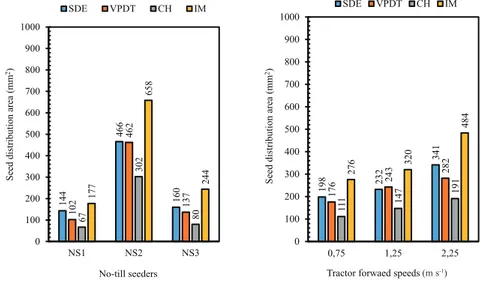
(a, b, c) means with the same letter are not significantly different From no-till seeder perspective, (NS1) and (NS3) sprinkled the seeds without distributing into a large area although (NS2) spread the seeds. For all the seeders the concave hull method calculated the smallest seed distribution areas. The NS2 machine spread the seeds about 3 times with respect to the other two machines.
All of the methods are dependent on the forward speed of the tractor. For the VPDT method area-speed relation seems to be distorted depending on the large areas produced by NS2 seeder. This
method has no filtering mechanism on the areas; voronoi polygons delaunay triangulation method tries to find the convex polygon enclosing all the points. When the seeds are widely spread on both horizontal and vertical axis, the area of the polygon will be larger. All of the experiments increasing the tractor forward speeds were increased seed distribution area (Figure 8).
Interaction values were given in Figure 9 and Figure 10. When examining the figures, maximum seed distribution area values were observed at the
sowing with NS2 no-till seeder and 2.25 ms-1 tractor
forward speed in all of the seed distribution area calculation methods.
For all the blocks, seeders and speed combinations, the concave hull algorithm resulted in the smallest area values. IM raised the widest areas almost in all blocks. Although in some cases SDE areas were smaller than the VPDT areas, VPDT generally brought about second smallest area values. The definition of concave hull foresees that area of the concave polygons would be smaller or equal to the areas of the convex polygons. Figure 10 illustrates some sets of seeds distributed.
144 466 160 102 462 137 67 302 80 177 658 244 0 100 200 300 400 500 600 700 800 900 1000 NS1 NS2 NS3 Se ed di str ibut ion a re a (m m 2) No-till seeders SDE VPDT CH IM 198 232 341 176 243 282 111 147 191 276 320 484 0 100 200 300 400 500 600 700 800 900 1000 0,75 1,25 2,25 Se ed di str ibut ion a re a (m m 2)
Tractor forwaed speeds (ms-1)
SDE VPDT CH IM
(m s-1)
Figure 8- Effects of no till seeders and tractor forward speeds on the seed distribution area Şekil 8- Anıza doğrudan ekim makinaları ve traktör ilerleme hızlarının tohum dağılım alanlarına etkileri
130
Ta r ı m B i l i m l e r i D e r g i s i – J o u r n a l o f A g r i c u l t u r a l S c i e n c e s 21 (2015) 123-131 79 177 332 485 694 814 206 223 266 0 100 200 300 400 500 600 700 800 900 1000 0,75 1,25 2,25 Se ed di str ibut ion a re a (m m 2)Tractor forward speeds (ms-1)
NS1 NS2 NS3
Integral (IM) method
(m s-1) 47 130 253 418 427 583 145 154 158 0 100 200 300 400 500 600 700 800 900 1000 0,75 1,25 2,25 Se ed di str ibut ion a re a (m m 2)
Tractor forward speeds (ms-1)
NS1 NS2 NS3
Standard deviational ellipse (SDE) method
(m s-1)
Figure 9- Effects of interactions on the seed distribution area for integral and standard deviation ellipse methods Şekil 9- İntegral ve elips yöntemine göre tohum dağılım alanına interaksiyonların etkileri
NS1 / V1 VPDT: 40.39 mm2 CH: 25.01 mm2 NS1 / V2 VPDT: 88.75 mm2 CH: 58.00 mm2 NS1 / V3 VPDT: 168.20 mm2 CH: 87.79 mm2 NS2 / V1 VPDT: 337.33 mm2 CH: 167.89 mm2 NS2 / V2 VPDT: 379.05 mm2 CH: 248.85 mm2 NS2 / V3 VPDT: 631.84 mm2 CH: 455.82 mm2 NS3 / V1 VPDT: 128.00 mm2 CH: 91.50 mm2 NS3 / V2 VPDT: 169.54 mm2 CH: 98.98 mm2 NS3 / V3 VPDT: 111.02 mm2 CH: 67.34 mm2
Figure 10- Effects of interactions on the seed distribution area for Voronoi and concave hull methods (dashed lines, convex hull used in VPDT method; continuous lines, concave hull; small circles, seeds) Şekil 10- Voronoi ve iç bükey zarf algoritması yöntemine göre interaksiyonların tohum dağılım alanına etkileri (kesik çizgiler Voronoi methoduna göre tohum dağılım alanı; sürekli çizgiler iç bükey zarf algoritması yöntemine göre tohum dağılım alanı; çemberler, tohumlar)
Düşey Düzlemdeki Tohum Dağılım Alanının Belirlenmesinde Yeni Bir Yaklaşım, Altıkat et al
131
Ta r ı m B i l i m l e r i D e r g i s i – J o u r n a l o f A g r i c u l t u r a l S c i e n c e s 21 (2015) 123-131
4. Conclusions
The coefficients of variation of the seeding depths of the seeders are all in acceptable limits. This means that No-till seeder with disc type furrow opener has the highest CV values while no-till seeder with hoe type furrow opener has the lowest ones. Increase in the tractor forward speed also causes an increase in the coefficients of variation of seeding depth.
No-till seeder with hoe type and winged hoe type furrow openers produced better results from the perspective of seed distribution area. Tractor forward speed also showed an important influence on seed distribution area; since speed increase created seed scattering, this rise on velocity raised area in which seeds distributed.
There exists three methods to evaluate seed distribution area; IM, SDE and VPDT. This research tried to show that the characteristic or concave hull method used in many other fields can be determinant of seed distribution area. CH method displays the characteristic of the distribution of points and the shape of the region and closer approach to the evaluation of seed distribution area. In the experiments, CH method produced the smallest seed distribution area values as expected.
Abbreviations and Symbols
NS1 no-till seeder with hoe type furrow opener
NS2 no-till seeder with disc type furrow opener
NS3 no-till seeder with winged hoe type fur-row opener
SDE standard deviational ellipse method IM integral method
VPDT Voronoi polygons with Delaunay triangu-lation method
CH concave hull method
References
Chen Y, Monero FV, Lobb D, Tessier S & Cavers C. (2004). Effects of six tillage methods on residue incorporation and crop performance in a heavy clay soil. Transactions of the ASAE 47(4): 1003−1010 Duckham M, Kulik L, Worboys M & Galton A (2008).
Efficient generation of simple polygons for characterizing the shape of a set of points in the plane.
Pattern Recognition 41: 3224 - 3236
ISO (1984). Sowing equipment, Test methods, Part 1: Single seed drills
Karayel D & Özmerzi A (2001). Effect of forward speed and seed spacing on seeding uniformity of a precision vacuum metering unit for melon and cucumber seeds.
Akdeniz University Journal of Faculty of Agriculture
14(2): 63–67
Karayel D & Özmerzi A (2007). Comparison of vertical and lateral seed distribution of furrow openers using a new criterion. Soil & Tillage Research 95: 69–75 Karayel D & Özmerzi A. (2005). Hassas ekimde
gömücü ayakların tohum dağılımına etkisi. Akdeniz
Üniversitesi Ziraat Fakültesi Dergisi 18(1): 139-150
Karayel D (2009). Performance of a modified precision vacuum seeder for no-till sowing of maize and soybean. Soil & Tillage Research 104: 121–125 Karayel D (2010). Sıraya Ekimde Yatay Düzlemdeki
Tohum Dağılımı ve Bitki Yaşam Alanının Voronoi Poligonlarıyla Değerlendirilmesi. Tarım Bilimleri
Dergisi-Journal of Agricultural Sciences 16: 97-103
Karayel D (2011). Direct Seeding of Soybean Using a Modified Conventional Seeder. Soybean Applications
and Technology, Rijeka - Croatia 3-18
Park J & Oh S (2012). A New Concave Hull Algorithm and Concaveness Measure for n-dimensional Datasets.
Journal of Information Science and Engineering 28:
587-600
Srivatsan RA, Viswanath AV & Ramanathan M (1998). Concave hull of freeform planar curves.
Chennai-600036
Wilkins D E, Kraft J M & Klepper B L (1991). Influence of plant spacing on pea yield. Transactions of the