Classification with overlapping feature intervals

(1)

3 2 . S - ¥

<îı;i· "? ;f,w Л - !.. Í.:· s ■ r- i йг* üJ» . - i ·&^ H-i t ^ij· SlS L·, I ύ'Ύ L Ш Ц I E..^.

a »iM Ψ * - іЦ uf· “ i !· ilâ

J flj . . M V *U(>· ** 4ıi>· ■■

" ΊΐΓ ИЛІ i ϊ 1 .T_• _bíH_{·ρ-3·.ί·} _{·.»· '*■}, 'Χ_,ς^ Λ I : ä :: ::: :« " ; > ■■·.- ·=: _■_J_^_J»_' _!_ц_5·_{It Ы.^4»·· :}_iu3_.1ІІГ.Ц, _{4<-â-i-¥r·}2?: ■:' M d t e s s iŞ fîi 4;i

■'! ',fî^‘J.: ;;ір^іу;іГ;ГІ1· i·:·' ı;l^-■-:'.;-î Ώ'ΙΪΙ'ϊ- ί

Лі· ■ ■ ІІ ЯІ'ІЯЬ ■ · И·· * я ··» -■«' ·ν·- *3· · ■■ .«■.·«·. · .«Μ: '<.· i*n « « ‘Otr·'···'» Μ >*■'«·«·-' ' ' . .*1^1.14.««»». . ‘«»|·, ·4β< Я **

(2)

CLASSIFICATIO N W IT H

O V E R L A P P IN G FEATUR E

INTERVALS

A THESIS

SUBMITTED TO THE DEPARTMENT OF COMPUTER ENGINEERING AND INFORMATION SCIENCE AND THE INSTITUTE OF ENGINEERING AND SCIENCE

OF BILKENT UNIVERSITY

IN PARTIAL FULFILLMENT OF THE REQUIREMENTS FOR THE DEGREE OF

MASTER OF SCIENCE

b y

Hakime Unsal Koç

(3)

j , ; : _

Assoc. Prof. H. Altay Güvenir (Advisor)

I certify that I have read this thesis and that in my opinion it is fully adequate, in scope and in quality, as a thesis for the degree of Master of Science.

Asst. Prof. Kemal Oflazer

I certify that I have read this thesis and that in my opinion it is fully adequate, in scope and in quality, as a thesis for the degree of Master of Science.

Asst. Prof. Ilyas Çiçekli

Approved for the Institute of Engineering and Science:

Prof. Mehmet BiâP^y Director of the Institute

(4)

G. -K63 1ЭЭ5

(5)

C L A S S IF IC A T IO N W IT H O V E R L A P P IN G F E A T U R E IN T E R V A L S

M .S . in Computer Engineering and Information Science Advisor: Assoc. Prof. H. A ltay Güvenir

January, 1995

This thesis presents a new form of exemplar-based learning method, based on overlapping feature intervals. Classification with Overlapping Feature Intervals (COFI) is the particular implementation of this technique. In this incremental, inductive and supervised learning method, the basic unit of the representation is an interval. The COFI algorithm learns the projections of the intervals in each class dimension for each feature. An interval is initially a point on a class dimension, then it can be expanded through generalization. No specialization of intervals is done on class dimensions by this algorithm. Classification in the COFI algorithm is based on a majority voting among the local predictions that are made individually by each feature.

Keywords: machine learning, supervised learning, inductive learning, incre mental learning, overlapping feature intervals, concept description

(6)

ÖZET

Ç A K IŞ IK Ö Z E L L İK A R A L IK L A R I İLE S IN IF L A N D IR M A

Bilgisayar ve Enformatik Mühendisliği, Yüksek Lisans Danışman: Doç. Dr. H. A ltay Güvenir

Ocak 1995

Bu tezde örnek-tabanh öğrenme için çakışık özellik aralıklarına dayalı yeni bir teknik sunulmuştur. Çakışık Özellik Aralıkları ile Sınıflandırma (COFI) bu yöntemin özel bir uygulamasıdır. Bu çıkarımsal, artımlı ve yönlendirilmiş öğrenme tekniğinde en temel gösterim birimi aralıktır. COFI algoritması tüm özelliklere ait her sınıf eksenindeki aralıkların izdüşümünü öğrenir. Aralıklar ilk olcU'cik sınıf eksenlerinde birer noktadırlar, daha sonra tüm bir eksen boyunca genelleştirmeyle genişlerler. Bu algoritmada herhangi bir özelleştirme gerçek leştirilmez. Öğrenme işleminden sonra, tahmin etme işlemi özelliklerin kendi adlarına yajDtığı tahminler arasındaki oy çokluğuna dayanır.

Anahtar Sözcükler: öğrenme, yönlendirilmiş öğrenme, çıkarımsal öğrenme, artımlı öğrenme, çakışık özellik aralıkları, sınıf tanımı

(7)

I would like to thank all people, especially to my family, who supported and encouraged me throughout this work. I would not have managed to finish this study and reach my goal without unfailing support and help of my fam ily. I would like to thank Anatolian University, Industrial Engineering, and Electrical L· Electronics Engineering Departments for providing me comfort able environment for my studies. I would like to express my gratitude to my advisor Assoc. Prof. H. Altay Güvenir for his valuable comments and endless help. Fincilly, special thanks to my husband. Özgür Koç, who has provided a motivating support and helped me to prepare and follow effective studying principles.

(8)

List of Figures

2.1 Classification of exemplai’-based learning algorithms. 10

2.2 An example concept description in the IBL algorithms in a do

main with two features. 11

2.3 An example concept description of the EACH Algorithm in a domain with two features... 15 2.4 An example concept description of the CFP Algorithm in a do

main with two features. 17

2.5 Constructing segments in CFP by changing the order of the

training dataset. 19

2.6 Constructing intervals in the COFI Algorithm with using same dataset as used in Figure 2.5 . 20

2.7 The NBC Algorithm. 26

2.8 Computing the a posteriori probabilities in the NBC Algorithm. 28 2.9 The NN* Algorithm... 30

3.1 An example of construction of the intervals in the COFI Algo rithm... 36 3.2 An example of construction of the intervals in the COFI Algo

rithm with the order of the training instances is changed. 37

(11)

3.4 Updating generalization distances in the COFI Algorithm. . . . 44

3.5 Training process in the COFI Algorithm. 46 3.6 Prediction process in the COFI Algorithm. 50 3.7 An example of execution of the prediction process in the COFI Algorithm. 51 3.8 An example of execution of the prediction process in the COFI Algorithm when test instance does not fall into any intervals. 53 3.9 An example concept description of the COFI Algorithm... 55

4.1 The concept description of the noise-free artificial dataset by the COFI Algorithm. 66 4.2 The concept description of the artificial dataset by the COFI Algorithm with one irrelevant feature. 67 4.3 Accuracy results of the COFI, the NN* and the NBC algorithms on domains with irrelevant attributes. 69 4.4 Memory requirement of the COFI, the NN* and the NBC algo rithms on domains with irrelevant attributes. 70 4.5 Accuracy results of the the COFI, the NN* and the NBC algo rithms on domains with unknown attribute values. 72 4.6 Memory requirement of the the COFI, the NN* and the NBC algorithms on domains with unknown attribute values... 73

A .l Concept description of the iris dataset... 91

A .2 Concept description of the glass dataset... 92

A.3 Concept description of the glass dataset - continued... 93

(12)

A .4 Concept description of the glass dataset - continued... 94

A .5 Concept description of the horse-colic dataset... 95

A .6 Concept description of the horse-colic dataset - continued. 96 A .7 Concept description of the horse-colic dataset - continued. 97 A .8 Concept description of the horse-colic dataset - continued. 98 A .9 Concept description of the ionosphere dataset... 99

A. 10 Concept description of the ionosphere dataset - continued. . . . 100

A .13 Concept description of the hungarian dataset... 103

A .14 Concept description of the hungarian dataset - continued...104

A. 15 Concept description of the Cleveland dataset...105

A .16 Concept description of the Cleveland dataset - continued...106

A. 17 Concept description of the wine dataset... 107

(13)

4.1 An overview of the real-world datasets. 7 5

4.2 Required memory and execution time of training for the COFI

Algorithm. 76

4.3 Accuracy results (%) of the algorithms for real-world datasets using leave-one-out evaluation technique. 77 4.4 Average memory requirements of the algorithms for real-world

datasets. 78

(14)

List of Symbols and Abbreviations

AI COFI c Ci Ct C4 C4.5 D f Deh e e-i E E j Rn f h 9 EACH GA GA-CFP H H f H f flower E f ¡upper i IBL IBl IB2 IB3 IB4 IBS Artificial Intelligence

Classification by Overlapping Feature Intervals Index of a class

Label of the zth class

Time constant of the training process of the COFI algorithm Decision tree algorithm

Decision tree algorithm

Generalization distance for feature / in the COFI algorithm Euclidean distance between example E and exemplar H An example

¿th example in the dataset An example

/t h feature value of the example E n-dimensional Euclidean space Index of a feature

¿th feature

Generalization ratio

Exemplar-Aided Constructor of Hyperrectangles Genetic Algorithm

Hybrid CFP Algorithm Hyperrectangle

/t h feature value of the exemplar H

Lower end of the range for the exemplar H for feature / Upper end of the range for the exemplar H for feature / Index of a training instance

Instance-based learning

Instance-based learning algorithm Instance-based learning algorithm Instance-based learning algorithm Instance-based learning algorithm : Instance-based learning algorithm

(15)

ID3 k KA log m max f mtUf ML n NBC n d i(f) NGE NN NN* P ( x k i ) P{Wc) P{wc\x)

R(ai,x)

V V / X Xi ^i,f W f Wh IR

A

\(ai,W j)

: Decision tree algorithm

Number of classes in the dataset Knowledge Acquisition

Logarithm in base 2

Number of training instcinces Maximum value for the feature / Minimum value for the feature / Machine Learning

Number of features in the dataset Naive Bayesian Classifier

Number of disjoint intervals for feature / Nested-Generalized Exemplars

Nearest Neighbor Algorithm

Special case of the Nearest Neighbor Algorithm

Conditional probability density function for x conditioned on given wj Prior probability of being class c for an instance

The posterior probability of an instance being class c given the observed feature value vector x

Conditional risk Vote vector

Vote vector of the feature /

The vote given to class c by feature / Instance vector

Value vector of Rh instance Value of feature / of instance i Weight of feature /

Weight of exemplar H

System whose input is training examples and output is 1-rule Weight adjustment rate of the CEP algorithm

(16)

Chapter 1 Introduction

Learning refers to a wide spectrum of situations in which a learner increases his knowledge or skill in accomplishing certain tasks. The learner applies inferences to soine material in order to construct an appropriate representation of some relevant aspect of reality. The process of constructing such a representation is a crucial step of in any form of learning [59].

One of the central insights of AI is that intelligence involves search, and that effective search is constrained by domain specific knowledge. This framework can be applied to problem solving, language understanding and learning from experience. One can even apply this search metaphor to machine learning as a field of scientific study [.38]. In this framework, machine learning researchers are exploring a vast space of possible learning methods, searching for techniques with useful characteristics and looking for relations between these methods.

Machine learning is one of the oldest and most intriguing areas of artificial intelligence and cognitive science. It has developed especially in 80’s, and has emerged as a subfield of AI that deals with techniques for improving the performance of a computational system. It is now distinguished from studies of human learning and from specific knowledge acquisition tools.

The aim of the machine learning and the statistical pattern recognition is to determine which category or class a given sample belongs to. Through an observation or measurement process, a set of values (usually numbers) which make up the observation vector serves as the input to a decision rule which

(17)

assigns the observed instance to one of the given classes [22]. In the statistical pattern recognition field, probabilistic approaches are used.

There are two kinds of major directions of AI research, symbolic and subsymbolic models. The most active research area in recent years has continued to be symbolic empirical learning. This area is concerned with creating with and/or modifying general symbolic descriptions, whose structure is unknown a -priori. Symbolic models are good in high-level reasoning, however they are weak in handling imprecise and uncertain knowledge. Subsymbolic models, such as neural networks and genetic algorithms, are powerful in lower-level rea soning especially imprecise classification and recognition problems. However, they are weak in high-level reasoning. Both of these models are important for understanding intelligent systems.

Learning fx'orn examples has been one of the primary paradigms of machine learning research since the early days of AI. Many researchers have observed and documented the fact that human problem solving performance improves with experience. In some domains, the principle source of expertise seems to be a memory for a large number of important examples. Attempts to build an intelligent (i.e., at the level of human) system have often faced the problem of memory for too many specific patterns. Researchers expect to solve this difficulty by building machines that can learn using limited resources. This reasoning has motivated many machine learning projects [48].

Inducing a general concept description from examples and counterexamples is one of the most widely studied method for symbolic learning. The goal is to develop a description of a concept from which all previous positive instances can be rederived while none of the previous negative instances can be rederived by the same process of rederivation of positive instances. Classificcition systems require only a minimal domain theory and they are based on the training instances to learn an appropriate classification function.

In this thesis, we propose a new symbolic model for concept learning, based on the representation of overlapping feature intervals. The Classification with Overlapping Feature Intervals algorithm is the particular implementation of this technique. In this new technique, overlapping concept descriptions are allowed, that is there may exist different classes for the same feature values. No specialization is done on the concept descriptions.

(18)

CHAPTER 1. INTRODUCTION

In the overlapping feature intervals technique, the basic unit of the rep resentation is an interval. Each interval is represented by four parameters: lower and upper bounds, the representativeness count, which is the number of instances that the interval represents and the associated class value o f the in terval. The intervals are constx'ucted through class dimensions for each feature. Initially, an interval is a point, that is, its lower and upper bounds are equal to initial feature values of the first instance for each feature. Then a point inter viú can be extended to a range interval such that its lower and upper bounds are not equal. This process is based on generalization through close interval heuristic [63]. During the training process, the set of values for each feature for each concept (class) is partitioned into segments (intervals) corresponding to concepts. That is, the concept description is the collection of intervals of each class dimension and the projection of these concept descriptions are learned by the COFI algorithm.

The ability to generalize from examples is widely recognized as an essential capability of any learning system. Generalization involves observing a set of training examples of some general concept, identifying the essential features common to these examples, then formulating a concept definition based on these common features. The generalization process can thus be viewed as a search through a vast space of possible concept definitions, in search for a cor rect definition of the concept to be learned. Because this space of possible conceiDt definition is vast, the heart of the generalization problem lies in utiliz ing whatever training data, assumptions and knowledge available to constrain this search.

Generalization is the main process of the training phase of the COFI algo rithm. The COFI algorithm does not use any specialization heuristic. In order to avoid overgeneralization of intervals, generalization is limited with a use of specified parameter. Therefore, the generalization of an interval to include a new training instance depends on the external variable, called generalization ratio and the maximum and the minimum feature value up to current exam ple. By using this generalization ratio and these local maximum and minimum feature values a generalization distance is calculated. Whether a feature Vcilue is joined to an existing interval or it constructs a separate point interval is determined by this generalization distance. Small generalization ratios cause many number of small intervals to be constructed, whereas hirge generalization

(19)

ratios cause small number of large intervals.

The prediction process is simply a search for the intervals corresponding to the test instance’s each feature value on the related class dimensions. If the test instance’s current feature value falls within an interval in at least one class dimension, then a prediction can be made. Otherwise, no prediction is made and the final prediction is UNDETERMINED.

In the prediction phase of the COFI algorithm, local knowledge of each feature is important and this knowledge is maintained in a vote vector. For each feature a vote vector, whose elements represent the vote given to each class by that feature,is constructed. The vote is the relative representativeness count., which is the ratio of the representativeness count of the matched interval to the total number of instances which have the same class value as the test instance. Then, each feature’s vote vector is summed for the final prediction. A voting is performed among the elements of this final vote vector, whose result is the class that receives the maximum vote in the final prediction of the COFI algorithm.

The COFI algorithm handles unknown attribute and class values in a straight forward way. Similar to human behavior, it just ignores these unknown attribute and class values. Most of the learning systems, usually overcome this problem by either filling in missing values with most probable vcilue or a value determined by exploiting interrelationships among the values of different at tributes or by looking at the probability distribution of known feature values [46|.

Here, we have firstly given the introduction of machine learning and de fined briefly the concept learning problem. Then an overview of the COFI algorithm has been presented. In Chapter 2, we will present some of the ex isting concept learning models. Then the detailed explanation about our new algorithm, COFI, will be given in Chapter 3. In Chapter 4, we evaluate the COFI algorithm by giving the complexity analysis and the results of empirical evaluation on artificial and real-world datasets. Finally, in Chapter 5, we will discuss the results of this study and conclude by giving general evaluation of the algorithm.

(20)

Chapter 2 Concept Learning Models

The field of machine learning (ML) is as difficult to define as its parent field artificial intelligence. One might describe it as the field of inquiry concerned with the processes by which intelligent systems improve their performance over time. However, such hard and fast definitions are no more successful at de scribing scientific disciplines than they are useful in characterizing everyday concepts. The best may be to describe the central tendency of the field, a tendency that may itself change as the field develops. For instance, machine learning shares with Artificial Intelligence (AI) a bias towards symbolic rep resentations rather than numeric ones, although symbolic representcition does not exclude the numeric one. Similarly, most machine learning research em ploys heuristic approaches to learning rather than algorithmic ones. These dimensions separate artificial and cognitive science from mainstream computer science and pattern recognition, and machine learning is much more closely associated with the former two areas than with the latter two.

Carbonell defines machine learning as follows [8]:

Perhaps the tenacity of ML researchers in light of the undisputed difficulty of their ultimate objectives, and in light of early disap pointments, is best explained by the very nature of the learning process. The ability to learn, to adapt, to modify behavior is an inalienable component of human intelligence.

Despite the name machine learning, a significant fraction of the field has 5

(21)

always been concerned with modeling human behavior, starting with Feigen- baum’s EPAM model of verbal learning [18]. There is also considerable inter est in applied machine learning research, focusing on the automatic construc tion of knowledge-based systems. For instance, Michalski and Chilausky have worked on a knowledge base from examples [36]. Since learning is a central phenomenon in human cognition, the researchers evaluate machine learning methods in terms of their ability to explain human learning.

A number of different themes can be identified within the machine learning community, each corresponding to central goals of its parent field, artificial in telligence. For instance, many AI researchers are concerned with implementing knowledge-intensive systems, nevertheless those often take many man-years to construct. Machine learning may provide methods for automating this pro cess, promising considerable savings in time and effort. Similarly, many AI researchers view artificial intelligence as a scientific discipline rather than an engineering one, and hope to formulate general principles of intelligent behav ior that hold accros a variety of domains. Since machine learning focuses on the acquisition of domain specific knowledge rather than the knowledge itself, it holds considerable potential for such general principles.

In the literature, two forms of learning can be distinguished: Knowledge Acquisition (K A) and Refinement o f Skills Through Experience [59].

1. Knowledge Acquisition: Briefly, knowledge acquisition, like machine

learning, describes techniques for increasing the functionality of a computer system. Knowledge acquisition focuses on the identification of knowledge for use in expert systems. Since this knowledge can be acquired in many ways, a wide variety of techniques have been studied. Knowledge acquisition and machine learning have been closely linked by their common application field, namely building up knowledge bases for knowledge-based systems. Learning and KA can be seen as two processes that construct a model of a task domain, including the systematic patterns of interaction of an agent situated in a task environment.

2. Refinement of Skills Through Experience: Learning in this per

spective, consist of gradually correcting deviations between observed and de sired behavior through repeated practice. This form of human learning covers

(22)

CHAPTER 2. CONCEPT LEARNING MODELS

mental, motor and sensory processes. For example, learning a musical instru ment is a good illustration of this process. Skill refinement is poorly under stood, and few AI systems have attempted to simulate it to date.

As scientific databases continue to grow, the analysis of scientific data be comes an increasingly important apj^lication area for machine learning research. Much of the research on scientific data is directed towards predicting properties of a physical process. Such processes are often described in terms of a function defined over the attributes of the domain or a stochastic model. First, the best machine learning technique is selected for the problem domain. It has been argued that instead of producing a description of the problem domain in terms of logical rules, functional descriptions or a complex statistical model, it is possible to store a collection of memories (cases) and perform prediction by interpolating from them. It is shown that memory-based reasoning meth ods [47] are as effective as the more complex approaches, such as probabilistic approaches.

Many decision-making problems fall into the general category of classifica tion. Empirical learning techniques for classification span roughly two cate gories: statistical pattern recognition [14, 22] and machine learning techniques for induction o f decision trees [43] or production rules. Although a technique from either category is applicable to the same set of problems, the two cate gories of procedures can differ radically in their underlying models and final format of their solution. Both approaches to learning can be used to chissify a sample pattern or example into a specific class.

Another distinction, symbolic and subsymbolic learning models concerns the level at which one represents instances and acquired knowledge. Many researchers in machine learning employ symbolic representations to describe both instances and rules [53]. In some cases, these involve complex logical or relational expressions, but a significant fraction of the work on inductive learning has employed attribute-value or feature representations of knowledge. However, inductive techniques also play a central role in subsymbolic learn ing paradigm, such as neural networks and evolutionary computing techniques [21, 40, 62]. In many cases, the inputs given to “subsymbolic” techniques are equivalent to the inputs provided to “inductive” methods.

(23)

symbolic induction methods. Their learning algorithms and representations of knowledge differ in significant ways, and their inductive biases also appear to be quite different. However, all can be applied to the same class of induction tasks, and they can be compared to one another both experimentally and analytically. In the following sections, we will explain some of the basic machine learning and statistical pattern recognition techniques applied to concept learning tasks.

Concept Learning

The most widely studied method for symbolic learning is one of inducing a general concept description from examples and usually known counterexamples of the concept. The task is to build a concept description from which cill pre vious i^ositive instances can be rederived by universal instantiation while none of the previous negative instances (counterexample) can be rederived by the same process [8]. Until recently “learning” referred almost exclusively to clas sification mechanisms, focusing on programs that learn concept descriptions from a series of examples and counterexamples. While learning now extends to include many other topics and types of systems, classification is still an active field. Classification systems have only a minimal domain theory and rely al most exclusively on the training examples to learn an appropriate classification function.

Learning a concept usually means to learn its description, that is, a relation between the name of the concept and a given set of features that are used to describe instances. Several different representation techniques have been used to describe concepts for supervised learning tasks. One of the widely used representation technique is the exemplar-based representation. The represen tation of the concepts learned by the exemplar-based learning techniques stores only specific examples that are representativeness of other similar instances.

Previous implementations of the exemplar-based models usually extend the the nearest neighbor algorithm, in which some kind of similarity or distance metric is used for prediction. Therefore, the training complexity of such al gorithms is proportional to the number of instances or objects stored. More recently, approaches using decision trees, connectionist circhitectures, represen tative instances, and hyperrectangles (exemplar-based learning) have appeared in the literature. These approaches construct concept descriptions by exam ining a series of examples, each of which is categorized as either a positive

(24)

example of the concept or a negative example (counterexample). That is, the main task is to construct a concept definition from the positive instances, which excludes the negative examples, by finding a relation between the name of the concept and a given set of features.

2.1 Exemplar-Based Learning

Exemplar-based learning was originally proposed as a model of human learning by Medin and Schaffer [35]. In the simplest form of exemplar-based learning, every example is stored in memory verbatim, with no change of representation. The set of examples that accumulate over time form category definitions; for example, the set of all chairs, that a person has seen, forms that person’s definition of “chair” . An example is normally defined as a vector of features, with values for each feature, plus a label which represents the category (class) of the example.

Exemplar-based learning is a widely used representation technique of the concept learning, in which the concept definition is constructed from the ex amples themselves, using the same representation language. In the exemplar- based learning, the examples are the concept. Little or no domain specific knowledge is required in exemplar-based learning.

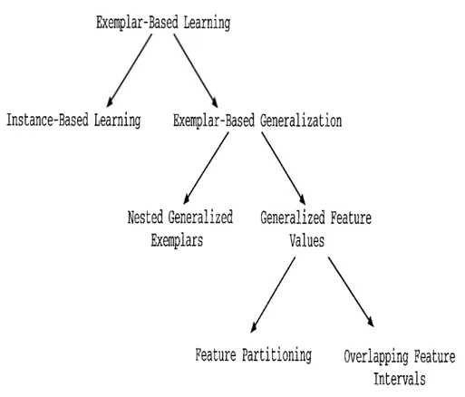
In the literature, there are many different exemplar-based learning models. A hierarchical classification of exemplar-based learning algorithms is shown in Figure 2.1. All of these models share the property that they use verbatim examples as the basis of learning. For example, instance-based learning [4] retains examples in memory as points, and never changes them. An example concept description of this representation is shown in Figure 2.2. The main implementations of this technique are performed by Aha and Kibler, and the algorithms are known as IBl through IB5 [2, 4]. The only decisions to be made are what points to store and how to measure similarity. Another example is the nested-generalized exemplars (NGE) of Salzberg. This model changes the point storage model of the instance-based learning and retains examples in the memory as axis-parallel hyperrectangles. Salzberg implemented NGE theory in a program called Exemplar-Aided Constructor of Hyperrectangles (EACH),

(25)

Exemplar-Based Learning

Instance-Based Learning

Exemplar-Based Generalization

Nested Generalized

Generalized Feature

Exemplars

Values

Feature Partitioning

Overlapping Feature

Intervals

Figure 2.1. Classification of exemplar-based learning algorithms.

where numeric slots were used for feature values of exemplar [49]. An exam ple of concept description is shown in Figure 2.3. In the feature partitioning techniques, examples are stored as partitions on the feature dimensions. One example of the implementation of feature partitioning is the Classification by Feature Partitioning (CFP) algorithm by Şirin and Güvenir [56]. An example concept description of this algorithm is presented in Figure 2.4. In the overlap ping feature intervals technique, intervals are the representation of the concept descriptions. In this technique, the main property is to allow overlapped con cept descriptions. The implementation of this technique is performed as the main purpose of this thesis and the algorithm is called Classification with Over lapping Feature Intervals (COFI).

2.1.1 Instance-Based Learning (IBL)

Instance-based learning algorithms use specific instances rather than precom piled abstractions during prediction tasks. These algorithms can also describe

(26)

₁₁

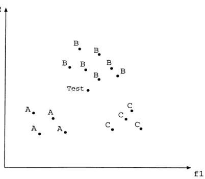
Figure 2.2. An example concept description in the IBL algorithms in a domain with two features.

probabilistic concepts because they use similarity functions to yield graded matches between instances.

IBL algorithms are derived from the nearest neighbor pattern classifier [10]. The primary output of the IBL algorithms is a concept description in the form of a set of examples. This is a function that maps instances to categories or classes.

In Figure 2.2, the representation of the concept description is shown. All ex amples are represented as points on the n-dimensional Euclidean space, where 12 is the number of features. In the figure, there are two features and three classes, namely A, B, and C. The test instance is marked as T est, and according to similarity function, this test instance will be classified as B.

An instance-based concept description includes a set of stored instances, called exemplars^ and some information concerning their past performances during classification. This set of instances can change after each training in stance is processed. However, IBL algorithms do not construct extensional concept descriptions. Instead, concept descriptions are determined by how the IBL cilgorithm’s selected similarity and classification functions use the current set of saved instances. There are three components in the framework which

(27)

describes all IBL algorithms as defined by Aha and Kibler [4]:

1. Similarity Function: computes the similarity between two instances,

similarities are real-valued.

2. Classification Function: receives the similarity function’s results and

the classification performance records of the instances in the concept description, and yields a classification for instances.

3. Concept Description Updater: maintains records on classification

performance and decides which instance to be included in the concept description.

Five instance-based learning algorithms have been implemented: IB l, IB2, IB3, IB4 and IB5. IBl is the simplest one and it uses the similarity function computed as

sim ila rity(x,y) — —

\

/=iE - S'/)'

(

2

.

1

)

where x and y are the instances and n is the number of features that describes the instances. IBl stores all the training instances. Therefore IBl is not incre mental, however, IB2 and IBS are incremental algorithms. IB2’s storage can be significantly smaller than I B l’s, as it stores only the instances for which the prediction was wrong. IBS is an extension of IB2. It employs a significance test to determine which instances are good classifiers and which ones are believed to be noisy. Once an example is determined to be noisy, it is removed from the description set. IBl through IBS algorithms assume that all attributes are equally relevant for describing concepts.

Extensions of these three algorithms [1, 2] are developed to remove some limitations which occur from some assumptions, such as, concepts are often assumed to

• be defined with respect to the same set of relevant attributes, • be disjoint in instance space, and

(28)

₁₃

IB4 [2] is an extension of IB3. It learns a separate set of attribute weights for each concept. These weights are then used in IB4’s similarity function which is a Euclidean weighted-distance measure of the similarity of two instances. Mul tiple sets of weights are used because similarity is concept-dependent, the sim ilarity of two instances varies depending on the target concept. IB4 decreiises the ciffect of irrelevant attributes on classification decisions. It subsequently is more tolerant of irrelevant attributes.

The problem of novelty is defined as the problem of learning when novel at tributes are used to help describe instances. IB4, like its predecessors, assumes that all the attributes used to describe training instances are known before training begins. However, in several learning tasks, the set of describing at tributes is not known beforehand. IB5 [2], is an extension of IB4 that tolerates the introduction of novel attributes during training. To simulate this capability during training, IB4 simply assumes that the values for the (as yet) unused at tribute are missing. During this time, IB4 fixates the expected I'elevance of the attribute for classifying instances. IBS instead updates an attribute’s weight only when its value is known for both of the instances involved in a classifica tion attempt. IBS can therefore learn the relevance of novel attributes more quickly than IB4. Theoretical analyses of instance-based learning algorithms can be found in [S].

Also noise-tolerant versions of instance-based algorithms are presented by Aha and Kibler in [3] in 1989. These learning algorithms are based on a form of significance testing, that identifies and eliminates noisy concept descriptions.

2.1.2 Nested-Generalized Exemplars (N G E )

Nested-generalized exemplar theory is a variation of exemplar-based learning. This theory is a model of a process whereby one observes a series of examples and becomes adept at understanding what those examples are examples of. Salzberg implemented NGE theory in a program called EACH (Exemplar- Aided Constructor of Hyperrectangles) [49], where numeric slots were used for feature values of exemplar. In EACH, the learner compares new examples to those it has seen before and finds the most similar example in memory. To determine the most similar hyperrectangle, a similarity metric, which is

(29)

inversely related to a distance metric (because it measures a kind of subjective distance), is used. This similarity metric is modified by the program during the learning process.

NGE theory makes several significant modifications to the exemplar-based model. It retains the notion that examples should be stored verbatim in mem ory, but once it stores them, it allows examples to be generalized. In NGE theory, generalizations take the form of hyperrectangles in a Euclidean n-space, where the space is defined by the variables measured for each example. The hyperrectangles may be nested one inside another to arbitrary depth, and in ner rectangles serve as exceptions to surrounding rectangles [49]. The learner compares a new example to those it hcis seen before according to similarity metric. The term exemplar (or hyperrectangle in NGE) is used to denote an example stored in memory.

The system computes a match score between E and / / , where E' is a new data point and H is the hyperrectangle, by measuring the Euclidean distance between these two objects. Consider the simple case where H is a point, representing an individual example. The distance is determined by the usual distance function computed over every dimension in feature space.

Deh = wh i

^ J? TJ

j - ( Wf

^ max f — min f y

(

2 .

2 )

where Wfj is the weight of the exemplar H, Wf is the weight of the feature / , E f is the value of the /t h feature on example E, H j is the value of the ft h feature on exemplar H, m ax/ and m in/ are the minimum and maximum values of that feature, and n is the number of features recognizable on E.

If the exemplar H is not a point but a hyperrectangle, as being the case usually, the system finds the distance from E to the nearest face of H. There are obvious alternatives to this, such as using the center of H. The formula used above is changed because i f / , the value of the /t h feature on i f , is now a range instead of a point value. If we let ii/./ower be the lower end of the range, and if/,upper be the upper end, then the equation becomes:

Deh — wh

df > [ W f_{--- ^—}

(30)

₁₅

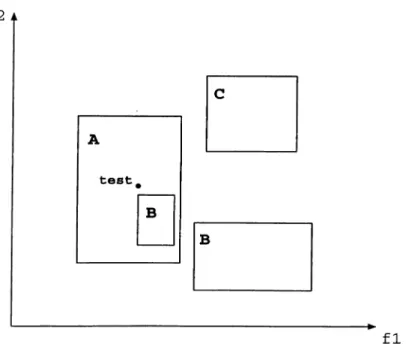
Figure 2.3. An example concept description of the EACH Algorithm in a domain with two features.

where df = E f Hj^upper E j Hj^uppgj· Hf¡lower E j E f <C. H j 0 otherwise (2.4)

If a training instance E and exemplar H are of the same class, that is, a correct prediction has been made, the exemplar is generalized to include the new instance if it is not already contained in the exemplar. However, if the closest example has a different class then the algorithm modifies the weights of features so that the weights of the features that caused the wrong prediction is decreased.

In Figure 2.3, an example concept description of EACH algorithm is pre sented for two features / i and /2. Here, there are three classes. A, B and C, and

their descriptions are rectangles (exemplars) as shown in Figure 2.3. It is seen in the figure that rectangle A contains another rectangle, B, in its region. B is an exception in the rectangle A. The NGE model allows exceptions to be stored quite easily inside hyperrectangles, and exceptions can be nested any number of levels. The test instance, that is marked as t e s t in Figure 2.3, falls into the rectangle A, so the prediction will be the class value A for this test instance.

(31)

2.1.3 Classification By Feature Partitioning

The Classification by Feature Partitioning (CFP) algorithm [56, 57, 58, 61] is similar to the COFI algorithm, and it is the basis of this thesis. In the CFP algorithm, learning is done by storing the objects separately in each feature dimension. These stored objects are disjoint segments of feature values. For each segment, lower and upper bounds of the feature values, the associated class, and the number of instances it represents, representativeness count, are maintained. CFP learns segments of the set of possible values for each feature. An example is defined as a vector of feature values plus a label that represents the class of the related example.

Initially, a segment is a point on the representing feature dimension. A segment can be extended through generalization with other neighboring points of the same class in the same feature dimension. In order for a segment to be extended to cover a new point in feature / , the distance between the segment and the value of feature / must be less than a given generalization limit, which is defined separately for each feature.

The CFP algorithm pays attention to the disjointness of the segments. However, segments may have common boundaries on different features. In this case, weights of the features are used to determine the class value. The feature which has the maximum weight is chosen and this feature determines the class value. The training process in CFP has two steps: learning feature segments and learning feature weights.

The prediction in CFP is based on a vote taken among the predictions made by each feature separately. The effect of the prediction of a feature in the voting is proportional to the weight of that feature. All feature weights are initialized to 1 before the training process starts. The predicted class of a given instance is the one which receives the highest amount of votes among all feature predictions.

The first step in the training is to update the partitioning of each feature using the given training example. For each training example, the prediction of each feature is compared with the actual class of the example. If the prediction of a feature is correct, then the weight of that feature is multiplied by (1 + A ) otherwise, it is multiplied by (1 — A ), where A is called the global feature

(32)

17

-EZZ2ZZZZ3-^13 - ^14

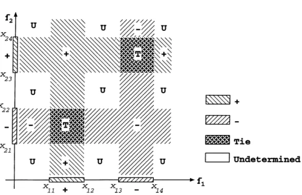
Figure 2.4. An example concept description of the CFP Algorithm in a domain with two features.

weight adjustment rate.

Figure 2.4 is presented here in order to illustrate the form of the resulting concept descriptions learned by the CFP algorithm with two features / i and /2. Assume that there are two classes, positive (+ ) and negative (-), and their

boundaries are shown in Figure 2.4. If a test instance falls into a region that marked with +, then the prediction will be the positive class for this instance in Figure 2.4. Similarly, if it falls into a region that marked with - , then the prediction will be the negative class. However, if the test instance falls into a region with marked with U, then no prediction will be made for this instance. Finally, if the test instance falls into a region that marked with T then the prediction will be made according to the weights of the features, that is, the feature which has the maximum weight makes its segment’s class value as the final prediction.

A noise tolerant version of the CFP algorithm has also been developed. In this extension, the CFP algorithm removes the segments that are believed to be introduced by noisy instances. A new parameter, called confidence threshold (or level) is introduced to control the process of removing the partitions from the concept description. The confidence threshold and observed frequency of

(33)

the classes are used together to decide whether a partition is noisy.

Also a hybrid system, called GA-CFP, which combines a genetic algorithm with the CFP algorithm has been developed [24]. The genetic algorithm is used to determine a very good set of domain dependent parameters ^ of the CFP, even when trained with a small partition of the data set. An algorithm that hy bridizes the classification power of the featui’e partitioning CFP algorithm with the search and optimization power of the genetic algorithm is presented. The resulting algorithm CA-CFP requires more computational capabilities than the CFP algorithm, but achieves improved classification performance in reasonable time. The complexity analysis of the CFP algorithm is presented in [25].

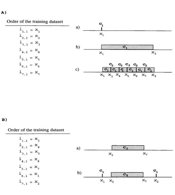
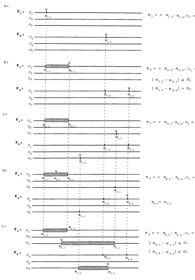
A limitation of the CFP algorithm can be seen in the following example in Figure 2.5. Here, the domain has only one dimension. In Figure 2.5A, the order of the training dataset is given. The first instance has the class value Cl and this instance constructs a point segment at the feature value Xi on the related feature dimension initially, as shown in Figure 2.5A.a. Then second

example is processed, it has also the class value Ci and its feature value is X2- Here, we assumed that the generalization distance is greater than the difference between a;i and X2· Therefore, a range segment is constructed on the feature dimension and its lower bound is Xi and upper bound is X2 as shown in Figure 2.5A.b. Then, let the next five instances belong to another class C2, and their

related feature values are between xi and X2- In this case, the big segment in Figure 2.5A.b has subpartitioned into six segments for class ci and no segment can be constructed for the second class C2 as shown in Figure 2.5A.C.

However, if the last five instances were processed before the first two in stances in the previous example, then the segments would have been con structed as shown in Figure 2.5B. Firstly, a range segment is constructed for the class C2 as shown in Figure 2.5B.a, and then two point segments are con

structed for the last two instances as in Figure 2.5B.b. The concept descriptions (segments) for A and B cases are very different from each other in Figure 2.5, although the same training instances were processed. It is seen that the order of the instances is very important and it affects the resulting concept description considerably.

In order to overcome this limitation, we need to store the instances of

(34)

CHAPTER 2. CONCEPT LEARNING MODELS ₁₉

A )

Order o f the training dataset

\ . l = ^2,1 = ^2 5 .1 = ^3 ^ , 1 = ^4 5 .1 = ^5 ^6.1 = "^6 5 .1 = ^7 a) b) c) mmmmm «=2 «=2 Ca Ca Ca Xi X, x^ B )

Order of the training dataset

1 1,1 = "^3 i 2,1 = ""4 i 3,1 = ^ 5 i 4,1 = ^ 6 i 5,1 = ^ 7 i 6,1 = i 7,1 = ^ 2 a) b) m mm m m m m m X7 X2

Figure 2.5. Constructing segments in CFP by changing the order of the training dataset.

(35)

Xi Xn

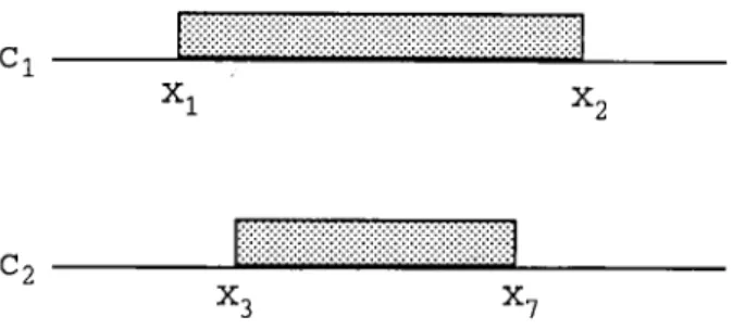
X, X - 7

Figure 2.6. Constructing intervals in the COFI Algorithm with using same dataset as used in Figure 2.5 .

different classes separately in a feature dimension independent from each other. The COFI algorithm solves this problem by storing examples as overlapping intervals for each class separately. The concept description learned by the COFI algorithm from the same set of training instances is shown in Figure 2.6 independent from the order of the examples, when the generalization ratio is chosen properly.

2.2 Decision Tree Techniques

Another approach to inductive learning is the one which involves the construc tion of decision trees. Here the concept representation is done by using tree structure.

A decision tree can be used to classify a case by starting at the root of the tree and moving through it until a leaf is encountered. At each non-leaf decision node, the outcome of the case for the test at the node is determined cind attention shifts to the root of the subtree corresponding to this outcome. When this process finally leads to a leaf, the class of the case is predicted to be that record at the leaf.

2.2.1 Decision Trees

This method was developed initially by Hunt, Marin and Stone in 1966 [27], and later modified by Quinlan (1979, 1983), who applied his IDS algorithm to deterministic domains such as chess and games [41, 42]. Quinlan’s later

(36)

CHAPTER 2. CONCEPT LEARNING MODELS ₂₁

research has focused on induction on domains that are uncertain and noisy rather than deterministic. His approach is to synthesize decision trees that has been used in a variety of systems, and he has described his system ID3, the

details can be found in [41, 42, 43]. A more extended version of ID3 is C4 . 5

[46] which can convert a decision tree to a rule base.

The overall approach employed by ID3 and C4.5 is to choose the attribute thcit best divides the examples into classes and then partition the data accord ing to the values of that attribute. This process is recursively applied to each partitioned subset, with the procedure terminating when all examjDles in the current subset have the same class. The result of this process is represented as a tree in which each node specifies an attribute and each branch emanating from a node specifies the set of possible values of that attribute. Terminal nodes (leaves) of the tree correspond to sets of examples with the same class or to cases in which no more attributes are available.

The recursive partitioning method of constructing decision trees will con tinue to subdivide the set of training cases until each subset in the partition contains cases of a single class, or until no tests offers any improvement. The result is often a very complex tree that “overfits the data” by inferring more structure than is justified by the training cases. A decision tree is not usually simplified by deleting the whole tree in favor of a leaf. Instead, the idea is to remove parts of the tree that do not contribute to classification ciccuracy on unseen cases, pi'oducing something less complex and thus more comprehensi ble. This process is known as the pruning. There are basically two ways in which the recursive partitioning method can be modified to produce simpler trees: deciding not to divide a set of training cases any further, or removing retrospectively some of the structure built up by recursive partitioning [46].

The former approach, sometimes called stopping or prepruning, has the attraction that time is not wasted assembling structure that is not used in the final simplified tree. The typical approach is to look at the best way of splitting a subset and to asses the split from the point of view of statistical significance, information gain, error reduction, or whatever. If this assessment falls below some threshold then the division is rejected.

The difference between this approach and the other learning methods, in cluding the COFI algorithm, is that the performance of these systems does not

(37)

depend critically on any small part of the model, whereas decision trees are much more susceptible to small changes.

2.2.2 IR System

In this section, the specific kind of rules, called “ 1-rules” , are examined. These are the rules that classify an object on the basis of a single attribute that is, they are 1-level decision trees. This system is defined by Holte, in 1993 [26].

IR is a system whose input is a set of training examples and whose out put is a 1-rule. IR can be treated as a special case of the classification with overlapping feature intervals technique. The COFI algorithm uses all of the featui'e infornuition for a final prediction. However, in IR, one of the features is chosen to make the final prediction. IR system treats all numerically valued attributes as continuous and uses a straight forward method to divide range of values into several disjoint intervals. Similar to the COFI algorithm, IR han dles the unknown attribute values by ignoring them. IR makes each interval “pure” , that is, intervals contain examples that are all of the same class. IR requires all intervals, except the rightmost, to contain a more than a predefined number of examples.

During the training phase, the construction of the intervals in the IR rule is done. After the training phase, one of the feature’s concept description is chosen as a rule.

Holte shows that simple rules such as IR are as accurate as more complex rules such as C4. Given a dataset, IR generates its output, a 1-rule, in two steps. First, it constructs a relatively small set of candidate rules (one for each attribute), and then it selects the one that makes the smallest error on the training dataset. This two steps pattern is similar to the training process of many learning systems.

In [26], Holte used sixteen datasets to compare IR and C4, and fourteen of the datasets were selected from the collection of datasets distributed by the machine learning group at the University of California at Irvine. The main result of comparing IR and C4 is an insight into the tradeoff between simplicity and accuracy. IR rules are only a little less accurate (3.1 percentage points)

(38)

CHAPTER 2. CONCEPT LEARNING MODELS ₂₃

than C4’s pruned decision trees on almost all of the datasets. Decision trees formed by C4 are considerably larger in size than 1-rules.

The fact that, on many datasets, 1-rules are almost as accurate as more complex rules has important implications for machine learning research and applications. The first implication is that IR can be used to predict the ac curacy of the rules produced by more sophisticated machine learning systems. A more important implication is that simple-rule learning systems are often a viable alternative to systems that learn more complex rules.

2.3 Statistical Concept Learning

The purpose of the statistical concept learning (or statistical pattern recog nition) is to determine to which category or class a given sample belongs to as for the machine learning. It is felt that the decision-making processes of a human being are somewhat related to the recognition of patterns; for example the next move in chess game is based upon the present pattern on the board, and buying or selling stocks is decided by a complex pattern of information. The goal of the pattern recognition is to clarify these complicated mechanisms of decision-making processes and to automate these functions using computers.

Pattern recognition, or decision-making in a broader sense, may be consid ered as a problem of estimating density functions in a high-dimension space and dividing the space into the regions of categories or classes. Because of this view, mathematical statistics forms the foundations of the subject.

Several classical pattern recognition methods have been presented in the literature [13, 14, 2 2, 62]. Some of them are parametric, that is, they are

based on assumed mathematical forms for either the density functions or the discriminant functions.

The Bayesian approach to classification estimates the (posterior) probabil ity that an instance belongs to a class, given the observed attribute values for the instance. When making a categorical rather than probabilistic classi fication, the class with the highest estimated posterior probability is selected.

(39)

The posterior probability, P(wc\x.) of an instance being class c, given the ob served attribute value vector x, may be found in terms of the prior probability of an instance being class c, P{wc)] the probability of an instance of class c having the observed attribute values, P { x ) . In the Naive Bayesian approach, the likelihoods of the observed attribute values are assumed to be mutually independent [14, 22, 60].

Naive Bayesian classifier is one of the common parametric classifiers. When no parametric structure can be assumed for the density functions, nonparamet- ric techniques, for instance nearest neighbor method, must be used for classifi cations. Here we will explain Bayes Independence (Naive Bayesian Classifier) and Nearest Neighbor methods because of their similarities to the COFI algo rithm.

Nearest neighbor method is one of the simplest methods conceptually, and is commonly cited as a basis of cornparison with other methods. It is often used in case-based reasoning [51].

Bayes rule is the optimal presentation of minimum error classification. All classification methods can be viewed as approximations to Bayes optimal clas sifiers. This theory is the fundamental statistical approach to the problem of ¡pattern classification. This approach is based on the assumption that the decision problem is posed in probabilistic terms, and that all of the relevant probability values are known.

Both NBC and NN algorithms are non-incremental, that is, they take and process all the training instances at once. On the other hand, the COFI algo rithm has an incremental structure. The COFI algorithm process each example separately and when new instances are fetched, it updates its concept descrip tion, that is, it does not have to know all the feature values at once. On the other hand. Naive Bayesian Classifier (NBC), and the version of nearest neighbor algorithm (NN*), similar to the COFI algorithm, process each feature separately. Therefore, we will compare the COFI algorithm with the NBC and the NN* algorithms.

(40)

CHAPTER 2. CONCEPT LEARNING MODELS ₂₅

2.3.1 Naive Bayesian Classifier (N B C )

The computation of the a posteriori probabilities P(tCc|x) lies at the heart of the Bayesian classification. Here Wc is the class and x is the feature vector of the instance to be classified. Bayes rule allows us to compute the probabilities P{wc) and the class conditional densities p(x|tOc), but since these quantities are unknown, the best is to compute P(tUc|x) using all of the information at disposal.

Let Cl = {u;i,u>2, . . ,uia:} be the finite set of s states of nature and A = {a i, q;2, .., « a } be the finite set of a possible cictions. Let be the loss

incurred for taking action ai when the state of nature is Wj. Let the feature vector X be a vector-valued random variable, and let p(x\wj) be the state-

conditional probability density function for x, that is, the probability density function for X conditioned on toj being the state of nature. Finally, let P{ wj)

be the a priori probability that nature is in the state P{wj). That is, P{ wj) is the proportion of all instances of class j in the training set. Then the a posteriori probability P(u;j |x) can be computed from p(x|iOj) by Bayes rule:

P{wj\yi) = p{x\wj)P{wj) P(x) (2.5) where i=l Wj). (2.6)

Since P{wj\yi) is the probability that the true state of nature is Wj, the expected loss associated with taking action cvj is merely

i?(ai|x) = ^ A (q; , >j) P (u;j|x). i=l

(2.7)

In decision theoretic terminology, an expected loss is called risk, and P(o;i|x) is known as the conditional risk. Whenever we encounter a particular observa tion X , we can minimize our expected loss by selecting the action that minimizes

the conditional risk. Now, our problem is to find a Bayes decision rule against P { w j ) such that minimizes the overall risk. A decision rule is a function a (x ) that tells us which action to take for every possible observation. That is, for

Classification with overlapping feature intervals

CLASSIFICATIO N W IT H

O V E R L A P P IN G FEATUR E

INTERVALS

ÖZET

Contents

List of Figures

List of Symbols and Abbreviations

R(ai,x)

A

Chapter 1

Introduction

Chapter 2

Concept Learning Models

2.1

Exemplar-Based Learning

Exemplar-Based Learning

Instance-Based Learning

Exemplar-Based Generalization

Nested Generalized

Generalized Feature

Exemplars

Values

Feature Partitioning

Overlapping Feature

Intervals

2.1.1

Instance-Based Learning (IBL)

11

\

(

.

)

13

2.1.2

Nested-Generalized Exemplars (N G E )

(

2

.

2

)

15

2.1.3

Classification By Feature Partitioning

17

2.2

Decision Tree Techniques

2.2.1

Decision Trees

2.2.2

IR System

2.3

Statistical Concept Learning

2.3.1

Naive Bayesian Classifier (N B C )

₁₁

₁₃

₁₅