Cost of Capital Estimation for Energy Network Utilities:
Revisiting from the Perspective of Regulators
Mustafa GÖZEN
12Abstract
Estimating the cost of capital for energy network utilities is critical because it directly effects decisions energy regulators make. The regulators have to estimate and allow a reasonable rate of return for network utilities as part of their duties under national laws, while balancing the protection of consumers and allowing an acceptable return to network investors. There is no generally accepted method applicable in all countries. Consequently, there is a need to review the estimation methods from the regulator's perspective, especially how to estimate an acceptable return if the network utility has an ownership structure with different return interests. Unfortunately, the available models provide either industry based or countrywide cost of capital values and do not consider different return expectations of network utility shareholders.
Keywords: Cost of Capital, Energy Regulation, Energy Utility JEL Classification Codes: G30, G32, G38
Enerji Şebeke Şirketleri İçin Sermaye Maliyetinin Tahmini: Düzenleme Kurumları Açısından İncelenmesi
Özet
Enerji şebeke şirketleri için sermaye maliyetinin tahmin edilmesi, enerji piyasası düzenleme kurumlarının aldıkları kararları doğrudan etkilediğinden kritik bir konudur. Enerji piyasası düzenleme kurumları, ulusal kanunlar ile belirlenen görevleri çerçevesinde, bir taraftan tüketicilerin haklarını diğer taraftan yatırımcılara kabul edilebilir getiri sağlayacak şekilde enerji şebeke şirketleri için makul bir getiri oranı belirlemek durumundadır. Tüm ülkelerde uygulanabilecek genel kabul görmüş bir tahmin yöntemi bulunmamaktadır. Özellikle farklı getiri beklentisine sahip ortaklık yapısına sahip enerji şirketi için sermaye maliyetinin tahmininin düzenleme kurumları
1
Dr. Energy Market Regulatory Authority, Electricity Market Department, Muhsin Yazıcıoğlu Cad. No.51/C Yüzüncüyıl 06530 Ankara, Turkey, email: [email protected].
2
I thank Dr. Subhes Bhattacharyya for his invaluable comments and recommendations on my research study that this article is based. In addition, I am grateful to Jean Monnet Scholarship Programme of the European Union for financing my stay in CEPMLP of Dundee University in the United Kingdom.
açısından incelenmesine ihtiyaç bulunmaktadır. Ancak mevcut tahmin yöntemleri ya endüstri bazında ya da ülke bazında sermaye maliyeti değerleri sağlamakta olup şebeke şirketlerinin hissedarlarının farklı getiri bekletilerini dikkate almamaktadır.
Anahtar Sözcükler: Sermaye Maliyeti, Enerji Düzenleme, Enerji Şirketleri JEL Sınıflandırma Kodları: G30, G32, G38
1. Introduction
Energy network business is regulated in most countries to prevent the unfair implementation of network connection and use of system charges. In general, the task of regulation is carried out by national regulatory agencies. The regulator is authorized by national laws to allow a fair and reasonable rate of return to the network utility while also considering the rights, and protecting the interests of customers. In this respect, the cost of capital is the key regulatory instrument for the energy regulator.
As discussed in detail in later sections, there is no method applicable in all countries. Different parties apply different methods with different interpretation of input data. This issue is a complex and difficult task for regulators in developing markets. Then there is an obvious need to review estimation methods from the regulator's perspective. Therefore, the main purpose of this article is to introduce key issues in estimating the cost of capital and emphasize the difficulties in the estimation.
This study is structured as follows. The second section covers the importance of, and main debates about the cost of capital in tariff regulation. The third section introduces and discusses methods for estimating the cost of capital. The fourth section explains the common methodology in setting the cost of capital. The fifth section evaluates the models from the regulator's viewpoint. The sixth section discusses whether the methods can be applied in developing markets and gives a short summary of approaches and models with global applicability. The seventh section calculates capital cost for two energy utilities in Turkey. The eight section makes some suggestions to regulatory agencies. Finally, the last section provides additional remarks and concludes the article.
2. Main debates about the cost of capital
Tariff regulation, basically, involves the regulation and monitoring of the wealth created by energy utilities through tariffs. Depending on the type of regulation, utilities are allowed to realize a certain level of profits. In order to accomplish regulatory targets and control the profits of regulated utilities, the
cost of capital becomes one of the key instruments. In this regard, the cost of capital is a powerful regulatory tool whether the rate of return or incentive based regulation is used as a regulatory policy (Grout, 1994).
As stated by Grout (1994), the role of the cost of capital is not the same for each regulatory regime. Under the rate of return regulation, the rate of return is set equal to the cost of capital. Although the cost of capital is one of the factors in the formulation of price and revenue caps, certain flexibility is given to the regulated utility. Therefore, the impact of cost of capital on the utility is expected to be relatively lower when the rate of return regulation is applied.
Furthermore, Rocha et al. (2007) highlight that regulator take great care in setting the rate of return under the price cap regime in highly volatile economies. According to Alexander and Irwin (1996), these realities present evidence for utilities regulated by incentive based regulation to require higher rates of return from their investments.
The typical tariff regulatory framework can be illustrated by means of the formula given below (Bosselman et al., 2000).
(1)
In Eq. 1, RR is the revenue requirement; OE is the total operating expenses including depreciation, OEadj is the expenses deductable for tax purposes, T is
the effective tax rate, Rd is the cost of debt, D is the quantity of debt, (Rd*D) is
the interest payable on the utility’s outstanding debt securities, RAB is the regulatory asset base, and R is the allowed return on RAB.
The product of (RAB*R) is intended to capture the cost of the capital invested in assets required to provide services. It is usually guided by the principle that the end result of its determination must be fair and reasonable from the viewpoints of both investors and consumers (Patterson, 1995). While it is critical to protect consumers from the pricing behavior of natural monopolists, the energy regulator has the duty to ensure that the utility can finance its operations and remain in business.
The regulatory agency has complete control over the allowed rate of return “R” when compared with other items in the revenue requirement formula (Crew and Kleindorfer, 1979; Bakovic et al., 2003). In other words, the regulator must balance the needs of consumers with the needs of investors to obtain fair returns on investment. Alexander et al. (2000) state that determining a fair and
RR
OE
R
D
*T
RAB*R
OE
reasonable level of allowed profits can lead to two situations. The first is the one that the utility will not want to invest under the allowance of low rate of return. The second is a situation where the utility will over-invest3 and/or make huge profits if a high level of return has been allowed (Averch and Johnson, 1962; Weyman-Jones, 1994).
In incentive-based regulation, rate of return considerations are implicit in setting and resetting the parameters. It is clear that regulators pay close attention to these issues when setting quality and efficiency parameters of incentive based regulation. Otherwise, shareholders will likely be unwilling to invest in sunk assets if they are only allowed to gain rates of return that are below the cost of capital. However allocative efficiency requires that the rate of return is equal to the cost of capital (Armstrong, et al., 1998).
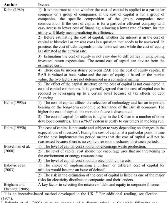
In addition to protecting the interests of both consumers and investors by tariff regulation, some authors underline the importance of factors summarized in Table 1 when estimating the cost of capital.
3
Table 1. Factors relevant to estimating the cost of capital
Author Issues
1) It is important to note whether the cost of capital is applied to a particular company or a group of companies. If the cost of capital is for a group of companies, the specific composition of the group companies need consideration. If the cost of capital is for a particular efficient company with easy access to lower cost of financing, allowing a lower rate of return for that utility will likely mean penalizing its efficiency.
2) Before estimating the cost of capital, whether the interest is in the cost of capital at historical or present costs is a question that needs to be answered. In practice, the cost of debt depends on the historical cost while the cost of equity is estimated at the current rate.
3) Estimating the cost of equity is not easy due to difficulties in anticipating investors' return expectations. The actual cost of capital can deviate from the estimated cost.
4) There can be inconsistency between RAB and the cost of equity capital. If RAB is valued at book value and the cost of equity is based on the market value, the two factors are not determined in a consistent manner.
Kahn (1989)
5) The effect of the capital structure on the cost of capital is not considered in cost of capital estimations. It is generally agreed that the cost of capital can be reduced by leveraging up to a certain level because of tax effects of debt financing.
1) The cost of capital affects the selection of technology and has an important bearing on the long-term economic performance of the British economy. The higher the cost of capital, the more the future is discounted.
Helm (1995a)
2) The cost of capital for utilities is higher in the UK than in a number of other developed countries. Thus RPI-Xa system is costly to customers in the long run. Helm (1995b) The cost of capital is not static and subject to vary depending on changes in the expectations of investorsb. Fixing the cost of capital at a particular point in time for the next implementation period means that the cost of capital will not be reassessed because there is no explicit revision mechanism between periods. 1) The level of capital cost should not encourage waste production.
2) The level of capital cost should not encourage uses that are threatening to the environment or energy resource base.
Bosselman et al. (2000)
3) The level of capital cost should protect public interests.
1) The choice of implementing a uniform or different cost of capital for utilities would become an issue of debatec.
Bakovic et al. (2003)
2) The risk in the estimation of the cost of capital is listed as one of the major risks for electricity distribution companies and their lenders.
Brigham and Ehrhardt (2005)
A key factor in selecting the mixture of debt and equity in corporate finance. a It is an incentive-based method developed in the UK. b For additional reading, see Gordon (1974).
c Bakovic et al. (2003) gives an example of a dispute raised in Colombia following the privatization of electricity distribution assets and in that dispute, the issue of implementing a uniform or different rate of return for utilities is debated among the concerned parties.
It is important to note that incentive based regulation does not lessen the importance of estimating the cost of capital, but requires careful thought and dynamic monitoring. The rate of return regulation allows that either the utility or the regulator opens discussion at any time to revise the allowed rate of return depending on market movements. This flexibility helps to protect the interests of utility investors under rate of return regulation.
However, as noted by Helm (1995b), incentive based regulation does not allow such an adjustment once the implementation period starts. Adverse market movements could significantly disrupt the profitability of the utility and result in lower return levels than investors' expectations. Being natural monopolies in their designated regions, energy network utilities must remain in business to ensure the uninterrupted supply of energy to end-users and the proper functioning of the market. This puts network utilities in a central position. Setting an attractive return at the beginning of each implementation period is an important task. But monitoring the utility's profitability becomes more critical when the market is volatile. Otherwise, the investment in network utilities would be more risky for investors. This is an issue that the regulators have to deal with in applying incentive-based regulation.
3. Estimation of cost of capital
For simplicity, the cost of capital can be broken into two main components: 1) the cost of debt and 2) the cost of money received by the utility in exchange for its stock or equity. The equity capital of a utility would be of two types: preferred and common. Since the earnings provided to both debt and preferred equity holders are usually known, common equity providers face the highest risk. Unlike debt and preferred equity, common stock holders are not entitled to any agreed or assured rate of return in advance on their investment. Common equity holders are paid from revenues after all debt and preferred investors of the utility have been paid. The remainder to common equity holders would be relatively low or even a negative value when compared to the level of risk they assume. For this reason, the cost of equity is difficult to measure.
Because the cost of equity is rarely observed directly from the market, it must be estimated and requires a forward-looking approach. Different methods can be used to calculate the cost of equity, such as comparative earnings, risk premium approach, Discounted Cash Flow (DCF), Capital Asset Pricing Model (CAPM) and Arbitrage Pricing Theory (APT) (Myers and Borucki, 1994).
3.1 Comparative earnings
In this method, the cost of equity is calculated based on book values of comparable companies. Nevertheless, it is not free of errors and disadvantages. First, it is difficult to find comparable companies since no two companies are identical even they are in the same business with the same shareholder structure. In addition, as stated earlier, the concept of cost of equity is market oriented. However, in this method, the cost of equity is calculated by using earnings based on book value. That is why this method provides cost of equity figures, which are independent from market movements.
Theoretically speaking, many comparative earnings ratios could be developed. However, in practice, the price-earnings ratio is frequently used. The expected earnings per share of the firms are multiplied by the appropriate price-earnings ratio based on the firm’s risk and industry to determine the appropriate price of the firm’s stock. Once the stock price is determined, the cost of equity is calculated by the same methodology of DCF. Although this method is easy to use, it is subject to some limitations when applied to emerging market stocks. The price-earnings ratio for a given industry may change continuously in these markets, especially when there are a few firms in the industry. Thus, it is difficult to determine the proper price-earnings ratio that should be applied to a utility in a developing market.
As pointed out by Madura (2008), the price-earnings ratio for a particular industry may need to be adjusted for the firm’s country, since the firm’s accounting guidelines and tax laws can influence reported earnings. Importantly, the implementation of price-earnings ratio is only possible under the assumption of efficient and perfect market conditions, which are lacking in developing markets.
3.2 Risk premium approach
In this approach, a risk premium is added to the long-term debt rate to calculate the cost of equity. The long-term debt rate can be obtained from the market. But there is still a need to estimate a premium reflecting the risk of equity. This approach is relatively easy to apply because only two parameters are needed. If the country issues the relevant debt instruments, then the only parameter required is the equity risk premium.
For matured markets, the data for equity risk premium is comparatively easy to determine in spite of controversial comments on the calculation of the
true equity premium. However, this data could be a burden for other markets. For this purpose, as an alternative, the study by Voll et al. (1998) regarding the cost of capital calculation for electricity distribution utilities in India sets the premium equal to the global market risk premium, assuming the U.S. market representing the global market. In addition, the study calculates the cost of equity by adding the cost of equity for a U.S. utility and the country risk premium.
3.3 DCF
DCF is the most widely used method to determine the cost of equity for regulated utilities in the U.S. In this method, the cost of equity is formulated as the expected rate of return demanded by investors in the regulated utilities’ equity capital. Then the rate of return is estimated as the sum of the current dividend yield and a long-term growth rate of dividends per share (Myers and Borucki, 1994).
The DCF formula is theoretically sound and simple to use, but it is obviously only applicable to utilities that pay dividends. It will give acceptable results only if the forecasted dividends grow at a constant rate infinitely. This assumption is criticized because no firm can grow forever at a rate exceeding the average growth of the economy (Franks and Broyles, 1979). On the other hand, Damodaran (2010a) points to the fact that the long-term expected growth rate is the most difficult parameter to estimate for emerging markets.
Based on simplifying assumptions, DCF is associated with practical problems and disadvantages. For example, Ross et al. (1993) argue that this approach is useless in many cases because the key assumption is that the dividend grows at a constant rate, which is unrealistic. Nevertheless, they show that the estimated cost of equity is very sensitive to the estimated growth rate. For example, an upward revision of the dividend growth rate of g by just 1% increases the estimated cost of equity by at least a full percentage point. Studies done by Brigham and Ehrhardt (2005) have shown that analysts’ forecasts represent the best source of growth rate data for DCF based cost of equity estimates. Since DCF provides results that are more accurate when the input data comes from the analysts, Ehrhardt (1994) suggests the use of such forecasts, if available.
Importantly, contrary to risk-return relation in finance, this method does not explicitly consider risk. Ross et al. (1993) point out that there is no direct adjustment for the riskiness of the investment under DCF. That means that no
allowance is made for the degree of certainty or uncertainty surrounding the estimated growth rate in dividends. As a result, it is difficult to say whether the estimated return meets the return expectations of the equity holders.
As the results of DCF are controversial, Makholm and Sander (1992) state that much of the disagreement in utility rate cases in the U.S. are about judgmental questions regarding the use of empirical data. Consequently, they conclude that DCF “… is a good tool that is often used poorly.”
Because of these problems, DCF is not recommended as the only method for the calculation. For example, Myers and Borucki (1994) investigate whether DCF could be used to estimate the cost of equity for regulated electric and gas utilities in the U.S. They calculate the cost of equities under several assumptions of dividend growth rates. Then they conclude that DCF results could not be used without cross checking the results obtained from other methods.
Apart from the problems caused by assumptions, the DCF formula requires adjustment considering real life. Makholm and Sander (1992) introduce four of the most common errors in the application of DCF that contribute to rate of return disputes and recommend the adjustment of the DCF formula. Table 2 summarizes the adjustments needed for the common errors as recommended by Makholm and Sander (1992).
Table 2. The adjustment of the DCF formula Common
errors
Description Adjustment of DCF formula
The ex-dividend date error
DCF assumes that common stock price of p is observed when the next dividend is on the ex-dividend date. Therefore it is necessary to remove the effect of nearer dividend payments from p. g p g 1 D r adj o adj ( ) *( ) 90 f f adj D T p p
radj is the adjusted cost of equity for
the ex-dividend date, p is the observed price of common stock,
padj is the adjusted common stock
price, Do is the quantity of the
previous dividend paid, g is the dividend growth rate, Tf is days until
next ex-dividend date, and Df is the
quantity of next dividend. The current
dividend yield error
In practice, the current dividend yield is multiplied by half the expected dividend growth rate to calculate the next period's dividend. The expected dividend payments over the next year should be calculated by multiplying the expected long-term dividend growth rate by dividend payments of the past periods.
The sustainable growth error
DCF assumes that the only source of equity financing is the retention of earnings. However, the issuance and the sale of new common stock at prices in excess of book value can also be a source of earnings growth for existing shareholders. ) ( ) (B*r S*V g av
B is the percentage of retained
earnings. rav is the expected return
on average equity. S is the funds raised from the sale of stock as a percentage of existing common equity. V is the percentage of funds raised from the sale of common stock that accrues to shareholders at the start of the period.
The flotation cost error
The issuance of common equity involves both direct expenses and underwritings fees. These costs are often measured as a percentage of the total common equity issuances.
g f 1 p g 1 D r o adj ) ( ) (
f is the flotation cost (%).
Source: Adapted from Makholm and Sander (1992). Note: the adjusted common stock price is the observed common stock price minus the accrued dividend.
3.4 CAPM
CAPM states that the cost of equity is the risk free return plus a risk adjustment. Risk adjustment is the product of the return on the market, as a whole, multiplied by the beta risk measure of the individual firm or project. According to CAPM, the relevant risk to be taken into account is not the total uncertainty of the investment in itself, but the contribution of the asset or project to the total risk of the firm’s cash flows, and ultimately to the risk of the shareholders' wealth (Hull, 1980; Sercu and Uppal, 1995; Harvey, 2001).
CAPM is complex and there are many implicit assumptions, both in CAPM itself and in its application. These include, among other things, market efficiency, the availability of reliable market betas, single periods, the beta of debt being zero, and a perfect market with no taxes and information costs, and rational and risk adverse investors with diversified portfolios (Northcott, 1995). CAPM could be formulated as the following.
(2)
In Eq. 2, Re is the cost of equity, Rf is the risk free rate, Rm is the market
premium, and βe is the beta of the subject equity relative to the market index.
Here the definition of the market depends on whether the relevant market is integrated or segmented. If integrated, investments are global and systematic risk is measured relative to a world market index. If capital markets are segmented, investments are made in a particular country and then systematic risk is measured relative to a domestic market index.
CAPM is theoretically sound and supported by academicians. However, there are debates regarding the nature of parameters to be used in CAPM. In addition, there are problems in applying CAPM to emerging markets where capital markets are not developed because CAPM requires inputs such as the risk free rate, beta, and the market risk premium. Beta and market risk premium are estimated using market data.
If the government in the emerging market does not issue debt instruments, the issue becomes more problematic. Then the question is what comparator data could be used. In practice, the international comparator data (mostly U.S. data) is used to meet the data requirement. Is this correct method? No, but it is widely applied. The use of the comparator data requires special attention because different markets apply different tariff regimes and countries issue different debt
m f
e f
e
R
β
R
R
instruments at different maturities. Therefore, the comparator data should be adjusted before use in the capital cost estimation.
3.5 APT
Like CAPM, APT assumes a linear relation between systematic risk and expected return. In contrast to CAPM, APT argues that many factors, not just beta, are important in explaining asset returns. As noted by Butler (2004), the main difference from CAPM is that APT takes a more general view of the types of risks that might be priced in the market. In this sense, CAPM is a specific form of APT. Therefore, in APT, a security`s expected return could be written as a linear function of n systematic risk factors (Eq.3).
(3)
In Eq. 3, Re is the cost of equity, Rf is the risk free rate, βn is the sensitivity
to factor n, and fn is the factor affecting expected return. Unfortunately, as stated
by Fifield et al. (2002), the theory is silent as regards to the number and types of these factors. While tests of these models have done much to increase our understanding of the manner in which assets are priced, much remains unclear.
Both CAPM and APT assume that the total variability of an asset’s returns can be attributed to two sources: 1) risks that influence all assets to some extent in the market, such as the state of the economy, and 2) other risks that are specific to a given firm, such as strikes. The former type of risk is usually named as systematic, non-diversifiable risk, or market risk, and the latter as unsystematic or diversifiable risk. Unsystematic risk is largely irrelevant to the highly diversified holder of securities. Nevertheless, no matter how well diversified a stock portfolio is, systematic risk, by definition, cannot be eliminated, and thus, the investor must be compensated for bearing this risk.
In addition to the above models, it is worthwhile mentioning an alternative model, the Fama and French`s three-factor model. Like CAPM and APT, this model assumes a linear relation between expected return and risk factors. In contrast, it uses three different factors for risk in the economy to estimate the cost of equity capital for a company: 1) market movements as in beta of CAPM, 2) the difference between the returns of small and big firms, and 3) high minus low book-to-market firms`returns (Franks, 2007; Pratt and Grabowski, 2008). Thus, Fama and French's model attempts to measure a company's return in
n n f
e R f f f
relation to these three coefficients for risks. The model can be formulated as the following.
(4)
In Eq. 4, Re , Rf , βe , and Rm represent the same variables as in CAPM. βz
and βd are the sensitivities of a security to a firm size and relative financial
distress factor respectively. fz is the difference in mean return between the
smallest 10% of firms and the largest 10% of firms. fd is the difference in mean
return between portfolios of firms with high and low ratios of book-to-market equity (Butler, 2004). The evaluation of these models, particularly from the perspective of tariff regulation, is discussed later.
4. The regulators' approach commonly used in estimating the cost of capital
The standard approach adapted by regulatory agencies is to use the weighted average cost of capital (WACC). Formally, WACC can be estimated by the following equations (5) or (6) depending upon choice:
(5)
(6)
In Eq. 5 and Eq. 6, Re is the cost of equity capital, Rd is the cost of debt, T is
the tax rate, and D and E are debt and equity ratios in a company. In practice, the cost of debt is usually estimated by adding a debt premium to the risk free rate (Jenkinson, 2006). However, the cost of equity is usually estimated by CAPM formula given below.
(7) d d z z f m e f e R β R R β f β f R ( )
tax e d pre*R
E
D
D
T
*R
E
D
E
WACC
(
1
)
1
R
T
E
D
D
R
E
D
E
WACC
posttax*
e*
d1
m f
e f
e
R
R
R
In Eq. 7, Rf is the risk free rate, βe is the equity beta, while (Rm-Rf) is the
market risk premium over the risk free return. βe is estimated by regression of
the utility's stock prices versus market index. Since the observed equity beta includes the effect of the capital structure, used before in Eq. 7, it is first unlevered and then relevered using the target debt-equity ratio by employing the following formula.
(8)
In Eq. 8, βa is the asset beta (unlevered beta) while βd is the debt beta. Often
in practice, a simplification is made and βd is typically assumed to be very small
or equal to zero. However, in general, it is estimated to have a value between 0.3 and 0.4 (Pratt and Grabowski, 2008). On the other hand, Arnold (2008) assumes a debt beta of 0.2-0.3 in his textbook. As an example, regulatory decisions assume a debt beta in the range of 0-0.28 in New South Wales in Australia (Independent Pricing and Regulatory Tribunal of New South Wales, 2002). Setting debt beta as zero means that the company can borrow at the risk-free rate. This assumption is not realistic, but usually used to find the unlevered asset beta (Northcott, 1995).
For the conversion of equity beta βe to eliminate the effect of the capital
structure, instead of Eq. 8, other conversion methods are also used. For example, Damodaran (2010b) makes corrections for cash in unlevered beta because cash and marketable securities have betas of around zero. For this purpose, Damodaran (2010b) uses the following formula. Unlevered Beta
corrected for Cash = Unlevered Beta/(1-Cash/Firm Value). The conversion
methods are listed and explained in Table 3.
E D E E D D e d a *
Table 3. Levered and unlevered beta conversion
Conversion Method Formula Assumptions
Hamada All risks are borne by
shareholders, βd is
zero, and debt has tax benefits.
Miles-Ezzell There is risk in the
timely realization of the tax deductions for the interest payments on debt.
Harris-Pringle The tax shield is more
risky.
Fernandez The ratio of debt to
book value of equity remains constant.
Practitioners' methods All risks are borne by
shareholders, βd is
zero, and debt has no tax benefits.
Source: Adapted from Pratt and Grabowski (2008). Notes: T is the effective tax rate,
D/E is debt-equity ratio, and Rd(pt) is the cost of debt prior to tax effect. aIt is a version of
the Hamada method under no tax benefits of debt.
In practice, Hamada and Practitioners' methods are mostly used (Ehrhardt, 1994). If debt beta is assumed not to equal to zero, then the Hamada method becomes as the following (Damodaran, 2003a).
(9)
In practice, the risk free rate is relatively easy to observe and the government debt instruments are generally accepted as risk free tools. The most controversial parameters of CAPM are the market risk premium and beta values. There are a large number of different viewpoints particularly about market risk premium. For example, Welch (2000a, 2000b) states that market risk premium can be different depending on the inputs used when estimating it, such as stock market indices, bonds, and historical time periods. Thus, he warns
E D T E D T d a e 1 (1 ) 1 E D d a a e ( ) a d a e T E D 1 E D a e 1 ) 1 ( ) * ( 1 ) ( ) ( ) ( pt d pt d d a a e R R T E D E D T a e 1 (1 ) users of market risk premium estimates to check which definition is used and the reason for the selection as well.
On the other hand, a survey by Bruner et al. (1998) for market risk premium used by practitioners in the U.S. provides that 37% of the respondents use a premium between 5-6%, and another 11% use an even lower value. Another survey by Welch (2008) reports that 1-year market risk premium and 30-year geometric market risk premium are about 5% at the end of 2007, and the sample interquartile range is 4% to 6%. Koller et al. (2005) recommends that the appropriate market risk premium be in the range of 4.5% to 5.5%.
5. Evaluation of the methods
The widely used methods of CAPM and DCF dominate in the estimation of cost of equity (Grout, 1994). In the UK, regulators mostly use CAPM (Jenkinson, 2006). On the other hand, recent surveys find that CAPM is by far the most widely used method, especially by large U.S. firms (Bruner et al., 1998; Graham and Harvey, 2001). In addition, almost 74% of respondents in one survey, and 85% in the other, state that they use CAPM (Brigham and Ehrhardt, 2005). However, there is a big variation in the implementation of CAPM among practitioners (Bruner et al., 1998).
The general application uses CAPM to assess the cost of equity and then uses DCF and other methods as a crosschecks (Franks, 2007). However, in practice, there is no doubt that, in estimating the cost of equity, both careful analysis and sound judgments are required (Brigham and Ehrhardt, 2005).
CAPM has two main advantages over other methods. First, it explicitly adjusts for risk. Second, it is applicable to companies whether they pay dividends or not. Thus, it may be useful in a wide variety of circumstances. Nevertheless, it has some disadvantages also. It requires that the market risk premium and the beta coefficient are estimated. Finally as with DCF, we essentially rely on the past to predict the future. When we use CAPM, economic conditions can change very quickly and past data may not be a good guide to the future (Ross et al., 1993).
In their empirical study for comparative computation of the cost of equity for regulated utilities, Roll and Ross (1998) conclude that APT provides a superior method, from both theoretical and pragmatic perspectives. They point out that CAPM has consistently underestimated the cost of equity for the utilities relative to their historic equity capital costs. Furthermore, they
demonstrate its application to a sample mixture of utilities from different sectors including energy, and derive much more sensible estimates of the cost of equity than those produced by CAPM.
In general, academics state that APT and the Fama and French's three-factor model provide a sounder theoretical basis than CAPM for determining the cost of capital. Moreover, it is a more sensible methodology for such computations in tariff regulation (Franks, 2007). In contrary, the survey conducted by Welch (2008) reports that for corporate capital budgeting purposes 75% of finance professors recommend CAPM, 10% recommend the Fama and French's three factor model, and 5% recommend an APT model.
Despite their theoretical strengths, APT and the Fama and French's three-factor model require a large amount of good quality data. Unfortunately, there are not enough empirical studies for its application in tariff regulation. Although theoretically acceptable, APT will not help energy regulators at least in the foreseeable future because there are still questions as to which parameters need to be inputted into APT formula.
6. Models for developing markets
The models discussed in detail in earlier sections work for mature markets, not for developing markets, mainly due to the unavailability or poor quality of the required data. For this reason, generally the modified or adjusted versions of CAPM are recommended to calculate the cost of equity in developing markets (Sabal, 2004; Harvey, 2005; Pereiro, 2006). The proposed models, essentially, suggest adding a country risk premium, or adjusting or modifying the beta, or using other risk parameters instead of beta in CAPM (Bekaert and Harvey, 2002; Sabal, 2004; Pereiro, 2006).
There are several suggestions on how to calculate the country risk premium. For example, Copeland et al. (2000) recommend the following. Country risk premium = (Country sovereign risk premium - credit risk premium - inflation differential). Country sovereign risk premium can be calculated as the difference between the interest rate on a local bond denominated in U.S. dollars and a U.S. government bond of similar maturity. Credit risk premium for a country's rated bond can be estimated by taking the difference between the yield to maturity on 10-year U.S. corporate bonds of the same rating with the country rated bond and the 10-year U.S. government bonds.
The major reasoning behind these versions are that developing markets pose greater risks to investors, and thus investors deserve additional premium for the risks they assume in developing markets. However, in recent years, this view has been questioned and it is argued that investment in developing markets actually reduces the risk attached to the overall cash flows of an international company (McRae, 1996). Moreover it provides opportunities for diversification benefits for the companies, due to the low correlation between developed and developing markets.
In practice, for tariff regulation in developing countries, country risk premium is added to the cost of equity calculated by CAPM for a proxy U.S. utility. Unfortunately, there is no literature suggesting the use of the other methods covered in earlier sections, such as the risk premium approach, APT, or the Fama Fama and French`s three-factor model, or even the use of DCF for regulatory purposes, probably due to the immature nature of capital markets in developing markets.
Pereiro (2001, 2006), Sabal (2004), Harvey (2005), and Estrada (2007) discuss some models with the global applicability. Among the models covered by these authors, some add sovereign risk premium instead of risk free rate in the CAPM formula. Some models add country risk premium to the cost of equity estimated for a U.S. utility using CAPM. Furthermore, some models use the relative volatility of the local market with regard to the U.S. market instead of beta of the CAPM. It is obvious that the models considering volatility as a parameter in the estimation will likely produce higher cost of capital values for countries with unstable markets.
The other model, the implied cost of capital, is based on finding the cost of equity by discounting cash flows to equity holders. This model assumes that the stocks are priced correctly. But, it is only applicable in efficient financial markets.
Another model suggested by Bekaert and Harvey (1995) includes the evolution of the financial integration between countries in the model. The model is based on a time-varying methodology. However, the difficulty is in calculating the degree of financial integration and including it in the formula. The dynamic model of Bekaert and Harvey (1995) is problematic because an incentive based tariff regime does not envision any adjustment in the tariff formula during the implementation period once the parameters are set at the beginning of the period. Another model, known as the Erb, Harvey, and
Viskanta Model (Erb et al., 1995; Erb et al., 1996), establishes a relation between the cost of equity and the country credit rating. This model could be an alternative for those markets with no stock exchanges. In addition, even the Arbitrage Pricing Theory has a strong theoretical acceptance, there is no clear guideline for the type and number of inputs to the model.
It is important to note that all the versions are developed to estimate the appropriate cost of capital for investments in the international setting from the perspective of investors in developed countries. This means that the proposed versions do not consider the return expectations of the local investors. On the other hand, finance theory clearly informs us that the cost of capital should reflect only non-diversifiable risk.
As also stated by Copeland et al. (2005), most agree that diversifiable risk is handled better in the cash flows. Thus adding country risk premium in the estimation formula is questionable, as it ignores the diversification effect of the investment. In the case of rate setting by regulators, the adjustment of the cash flow for non-diversifiable risk could only be done by increasing allowed revenues to the utility. Nevertheless, the adjustment of the revenues would not be a solution if the utility has different shareholders with different return expectations.
Even though a large number of models have been developed for the international setting, there are no common approaches accepted by academicians and practitioners. For example, Sercu and Uppal (1995) advise to check first whether or not there is integration between the concerned markets. According to the integration status, either the local CAPM for the country or the international CAPM would be selected. The local CAPM uses the beta value calculated by the local common stock return against the local market index. On the other hand, the international CAPM uses the beta value calculated by the local common stock return against the international market. Although some institutions produce international market indexes (For instance, MSCI World index), in practice, the U.S. market is taken as proxy for the international market.
Having chosen the model, then the next stage is to obtain estimates of the model parameters. In contrast, Shapiro (2003) recommends a pragmatic approach for U.S. based companies to measure the betas of international operations against the U.S. market portfolio, due to the quality of U.S. capital market data derived over a long period of time.
In contrast, Sabal (2004) argues that what is important is not the degree of integration, but whether the investor concerned is locally or globally diversified. Sabal (2004), however, does not answer the question regarding which shareholders one is supposed to look at in order to analyze their degrees of diversification. In practice, there are utilities whose direct shareholders are not diversified at all, but their indirect shareholders are diversified at the national or global level. In essence, in energy utilities, the controlling owners do not appear as direct shareholders. In many cases, they are indirect shareholders.
As regards the proposed versions of CAPM, there is no agreement as to which model has a theoretical background and could be applied with confidence in developing countries. In summary, we can say that, in practice and theory, there are different implementations and proposals, which do not provide clear and cohesive guidelines for regulators in developing markets.
7. Capital cost calculations for Turkish energy companies 7.1 Calculation methodology and input data
In this article, capital cost is calculated for two electricity companies. The first one is Zorlu Enerji Elektrik Üretim A.Ş. (ZOREN), which is electricity generator whose shares are traded in Istanbul Stock Exchange (ISE). The second is regional electricity distribution companies. In Turkey, there are 21 regional electricity distribution companies. EMRA - Turkish energy regulator - regulates the distribution services of these utilities and allows them to gain a certain rate of return by tariff regulation. Privatization procedures for 12 electricity distribution utilities are completed and procedures for others are continuing.
For calculation purposes, the real pre-tax WACC approach (Eq.5) is used to estimate the cost of capital for these two utilities. For electricity distribution utilities, a sectoral cost of capital is estimated instead of calculating capital cost for each utility. The reason is that none of regional distribution utilities are publicly traded company. In addition, it is difficult to find the required data and differentiate the input data among the utilities. In order to estimate the cost of equity, four models applicable to Turkey are selected and listed in Table 4.
Definitions of symbols and parameters used in Table 4
Symbol/Parameter Definition
Re The cost of equity
Rfu , Rfw , Rs The U.S. risk free rate, the global risk free rate, and the
sovereign spread respectively
Rmu , Rmw The U.S. market return, and the global market return
respectively
βu The beta of the U.S. company computed against the U.S.
market index
Rc The country risk premium
Table 4. List of selected models applicable to Turkey
Models Source Cost of equity formula and short description
Country risk premium (Rc) is added to the
CAPM formula instead of the U.S. market risk premium of (Rmu-Rfu)
Sabal, 2004 Re=Rfu+βuRc
The Beta Approach Re=Rfu+βu(Rmu-Rfu+Rc)
The Bludgeon Approach
Damodaran, 2003a, 2003b, 2009a, 2009b
Re=Rfu+βu(Rmu-Rfu)+Rc
The Goldman Sovereign Spread Model
Mariscal and Lee, 1993; Harvey, 2005
Re=Rs+βw(Rmw-Rfw)
1) The cost of equity is calculated by adding the country long-term debt rate and the global market risk premium. Risk Premium Approach Voll et. al.,
1998
2) The cost of equity is calculated by adding the cost of equity for a U.S. utility and the country risk premium.
The cost of debt is calculated by adding a margin over the risk free rate for Turkey. For example, 10-year Turkish Eurobonds issued in US$ is taken as a reference and a certain debt premium is added to the average rate of this debt instrument to arrive at a cost of debt figure for energy utilities.
In general, the rate of a government issued debt instrument is accepted as a risk free rate. Because the international debt instrument implicitly includes a sovereign premium, the sovereign premium is subtracted from the rate of the Turkey’s Eurobond and the long-term future inflation differential between
Turkey and the U.S. is added to arrive at a risk free rate for Turkey (Copeland et al., 2000).
As a U.S. risk free rate, the rate of the 10-year U.S. Government bond is used. The average rate of 10-year U.S. Government bond for the last 12 months is about 2.75% (Wall Street Journal, 2011). It is assumed that the U.S. risk free rate represents the world risk free rate and the U.S. market risk premium represents the world market risk premium.
In calculations, the nominal pre-tax WACC is calculated by using Eq.5. Then this value is converted to the real pre-tax WACC by using the adjusted Fisher formula. The formula can be written as (1+nominal-pre tax WACC) = (1+real pre-tax WACC value) x (1+expected inflation).
The risk free rate for Turkey is calculated by taking the arithmetic average of Eurobonds in US$ issued in 2010 and 2011 and the result is 5.83%. The arithmetic average of the spreads for the same bonds during the same period is taken as sovereign spread and calculated as 2.04%. This value is also taken as country risk premium.
The sovereign spread of 2.04% is subtracted from the rate of the Turkey’s Eurobond of 5.83% and the long-term future inflation differential between Turkey and the U.S. is added to arrive at a risk free rate for Turkey. Then a risk free rate of 6.79%4 for Turkey is calculated (Copeland et. al., 2005; Central Bank of the Republic of Turkey, 2011; InflationData.com, 2011). The long-term future inflation rate differential between Turkey and the U.S. is assumed to be 3.0, considering the inflation performance of both countries in the last 10 years and the inflation rate forecasts5.
The cost of debt is calculated by adding debt premium to the risk free rate for Turkey. Debt premium is assumed as 1.50%, considering corporate bond spreads over U.S. Treasury Bonds. Furthermore, in practice, a debt premium of 1.50% has widespread acceptance (Damodaran, 2010b).
From the studies and comments in Koller et al. (2005) and Welch (2008), market risk premium is reported at most 6%. The Federal Reserve Bank of Cleveland (2011) reports that its latest estimate of 10-year expected inflation is 1.83%.
4
It is the result of (5.83 - 2.04 + 3.00). 5
The inflation data for Turkey is obtained from the internet site of Central Bank of the Republic of Turkey and the U.S. inflation data is obtained from InflationData.com.
Since there is no listed electricity distribution utility in ISE, the comparator data is used for beta value. In general, asset beta for electricity distribution utilities ranges between 0.35-0.50. For example, Independent Pricing and Regulatory Tribunal of New South Wales (2002) reports an asset beta of 0.35-0.50 for Australian electricity distribution utilities and Damodaran (2010c, 2010d) calculates asset beta of 0.46-0.49 for electricity utilities in different regions of the U.S. Since electricity distribution utilities under incentive-based regulation face more risk, the highest value of the range is used in calculations.
On the other hand, the shares of ZOREN - the selected electricity producer - have been quoted in ISE since May, 2000. Because there are no good quality data series for beta calculations, the comparator data for the beta value is also used for ZOREN. As a comparator data, an asset beta of 0.70 for ZOREN is used in the calculations (Damodaran, 2010c; Damodaran, 2010d).
Asset beta values are converted to equity beta values using the Hamada conversion method used before in the selected cost of equity models (See Table 3).
Even though there is room for tax benefits from higher leverage, half of the capital structure of the utilities is foreseen as equity. Therefore, the beta applied to utilities reflects the target gearing.
The parameters used in the calculations are summarized in Table 5.
Table 5. List of parameters
Parameters Value
Electricity Distribution Co.
ZOREN
Risk free rate for Turkey (%) 6.79 6.79
Risk free rate for the U.S. (%) 2.75 2.75
Debt premium (%) 1.50 1.50
Cost of debt (%) (6.79 + 1.50) 8.29 8.29
Market risk premium (%) 6.00 6.00
Asset beta (unlevered beta) 0.50 0.70
Equity beta (levered beta) 0.90 1.26
Debt/equity ratio (%/%) 50% / 50% 50% / 50%
Country risk premium/sovereign risk (%)
2.04 2.04
Statutory tax rate (%) 20 20
10 year expected inflation rate for the U.S. (%)
1.83 1.83
Long-term inflation rate difference for Turkey and the U.S. (%)
7.2 Results and discussion
Cost of capital estimation results are summarized in Table 6. Table 6. Weighted average cost of capital estimates
Real pre-tax WACC (%) Model Formula for estimating cost of equity Electricity Distribution Co. ZOREN Rc is added instead
of the U.S. market risk premium. Re= Rfu+βuRc 5.09 5.54 Beta Approach Re=Rfu+βu(Rmu-Rfu+Rc) 8.41 10.18 Bludgeon Approach Re= Rfu+βu(Rmu-Rfu)+Rc 8.52 9.85 The Goldman Sovereign Spread Model Re=Rs+βw(Rmw-Rfw) 6.84 8.17 1) Re= Rfl+(Rmu-Rfu) 10.12 10.12 Risk premium
approach 2) Re for a utility in
Turkey=Re for a utility
in the U.S.+Rc
8.52 9.85
As seen from Table 6, the results of risk premium approach -1 for both companies are the same, which is unrealistic because two utilities have different beta values. This specific method does not consider the differences in risk profiles of the utilities. In addition, the model based on addition of a country risk premium instead of the U.S. market risk premium provides unrealistic results for both utilities, which are even below the risk free rate for Turkey. The Goldman Sovereign Spread Model provides a result for electricity distribution utility, which is very close to the risk free rate for Turkey. Except for the results below the cost of debt and, of the risk premium approach -1, the real pre-tax WACC for electricity distribution utility changes from 8.41% to 8.52% and for ZOREN from 9.85% to 10.18%.
8. Policy guidelines to regulators
From a finance point of view, the cost of equity capital is viewed as an opportunity cost. This is the return that the investor would expect to make on other investments of similar risk. The cost of capital value is not an exact value because it requires forward-looking and subjective evaluation. Importantly, it is based on the investors` risk profile. Hence, it is wrong to calculate a single cost
of capital value. It is better to estimate the cost of capital value in a range with lower and higher figures (Sabal, 2004; Arnold, 2008).
Arnold (2008) argues that precision is less important than knowledge about the reasonable range and he recommends focusing on estimating the boundaries for the range of values. The minimum value of the range must be set, at least, at a value to encourage the interested parties to invest in the sector. On the other hand, the maximum value must be set, at most, at the highest value that could be earned from alternative investments in a competitive market (Kahn, 1989).
CAPM based models only estimate the minimum cost of capital values and do not recommend any maximum value. If a country is facing security of energy supply or is projected to face a shortage in terms of network investments, regulators should allow a reasonable return in order to maintain the interests of the existing shareholders, and attract more investment to the sector.
In setting the cost of capital, energy regulators should review other cost of capital values determined by, if any, other regulators in the home country and cooperate with them. The difference between the estimated costs of capital among regulated energy and non-energy utilities of similar risks would negatively affect the investment flow among sectors. As proposed by Mayer and Franks (Franks, 2007), one solution would be to appoint a standing committee that would review new evidence for cost of capital estimation and provide regular updates both on existing and new models, and estimate the relevant variables required for the models.
Different investors probably have different expected rate of returns, since they see different amounts of risk in the same investment. The various versions of CAPM assume a homogenous and rational shareholder structures with diversified portfolio, and do not give answers for shareholder structure with different return expectations. Therefore, according to the assumptions of the standard CAPM, the shareholders of energy utilities and their portfolio strategies are more important than the degree of market integration. This is important because energy regulators should first identify the shareholders of energy utility and identify whether they diversify away their unsystematic risk or not. Even if this approach is accepted, some questions remain unanswered. Will the regulator be required to evaluate only direct shareholders of the utility or all shareholders behind direct shareholders, until all indirect shareholders are real persons in the utility’s ownership structure? Assuming that all direct and indirect legal entity shareholders are not diversified and only the indirect
individual shareholders have diversified portfolios, in this case, which shareholders will be counted in the analysis? To make it clear, at what level of shareholders will regulators evaluate whether shareholders are diversified or not? This will certainly burden regulators who will have to collect the information needed for this type of analysis.
In risk-return relations, what matters is not the energy utility itself. As stated earlier, it is the shareholders of the utility that matter most, whether they are diversified locally or globally (Sabal, 2004). As long as the shareholders of two utilities are not exactly the same, the estimated cost of capital for these utilities would likely be different, subject to other things being similar in the utilities. Therefore, it is not logical to apply the same rate of return value to all utilities and each utility must be treated differently.
9. Concluding remarks
Cost of capital is a hot issue in finance. Approaches and suggestions in either theory or practice in setting a cost of capital for energy utilities do not provide clear answers or guidelines for energy regulators. Nevertheless, regulators are authorized to allow a fair rate of return to energy utilities while taking necessary measures to protect consumers. The available models estimate cost of capital figures on an industry basis or countrywide. This will be irrelevant if the network utility is not owned wholly by the same shareholders or the shareholders of the network utilities are not homogenous in terms of return expectations. However, regulators need to consider differences if the network utility has shareholders with different risk return expectations. Unfortunately, there is no clear solution to solve this challenging issue. How to harmonize different return expectations is an area that requires further thought and research.
References
Alexander, I., Estache, A., and Oliveri, A., (2000), A few things transport regulators should know about risk and the cost of capital. Utilities Policy, 9, 1-13.
Alexander, I. and Irwin, T. (1996), Price Caps, Rate-of-Return Regulation,
and the Cost of Capital, Note No.87, September, Washington, D.C.: The World
Armstrong, M., Cowan, S., and Vickers, J. (1998), Regulatory reform:
Economic analysis and British experience, fourth printing. Cambridge, MA:
The MIT Press, Massachusetts Institute of Technology.
Arnold, G. (2008), Corporate Financial Management, fourth edition. England: Pearson Education Limited.
Averch, H. and Johnson, L.L. (1962), Behavior of the firm under regulatory constraint, The American Economic Review, 52(5), 1052-1069.
Bakovic, T., Tenenbaum, B., and Woolf, F. (2003), Regulation by contract:
A new way to privatize electricity distribution? Washington, D.C.: The World
Bank.
Bekaert, G. and Harvey, C.R. (1995), Time-varying world market integration, Journal of Finance, 50, 403-444.
Bekaert, G. and Harvey, C.R. (2002), Research in emerging markets finance: Looking to the future, Emerging Markets Review, 3, 429-448.
Bosselman, F., Rossi, J., and Weaver, J.L. (2000), Energy, Economics and
the Environment, New York: Foundation Press.
Brigham, E.F. and Ehrhardt, M.C. (2005), Financial Management: Theory
and Practice, eleventh edition, Australia; United Kingdom: Thomson &
Southwestern.
Bruner, R.F., Eades, K.M., Harris, R.S., and Higgins, R.C. (1998), Best practices in estimating the cost of capital: Survey and synthesis. Financial
Practice and Education, 8, Spring/Summer, 13-28.
Butler, K.C. (2004), Multinational Finance, third ed., Mason, Ohio: Thomson & South-Western.
Central Bank of the Republic of Turkey (2011), Inflation rates for Turkey, in Turkish, <http://www.tcmb.gov.tr>, 18.08.2011.
Copeland, T.E., Koller, T., and Murrin J. (2000), Valuation: Measuring and
Managing the Value of Companies, New Jersey: John Wiley & Sons, Inc.
Copeland, T.E., Weston, J.F., and Shastri, K. (2005), Financial Theory and
Corporate Policy, fourth edition, Boston: Pearson Addison Wesley.
Crew, M.A. and Kleindorfer, P.R. (1979), Public Utility Economics, London: The MacMillan Press Ltd.
Damodaran, A. (2003a) Valuation in emerging markets, Choi, F.D.S. (ed.),
International Finance and Accounting Handbook, Third Edition, John Wiley &
Sons, Inc., New Jersey, Chapter 9.
Damodaran, A. (2003b) "Country risk and company exposure: Theory and practice", Journal of Applied Finance, Fall/Winter: 63-76.
Damodaran, A. (2009a) "Volatility rules: Valuing emerging market companies", September, http://pages.stern.nyu.edu/~adamodar/pdfiles/ papers/emergmkts.pdf, (24.06.2010).
Damodaran, A. (2009b) "Equity risk premiums (ERP): Determinants, estimation and implications", October 22, http://papers.ssrn.com/sol3/ papers.cfm?abstract_id=1492717, (22.06.2010).
Damodaran, A. (2010a), Measuring country risk,
<http://www.qfinance.com/contentFiles/QF01/g4fqn4jz/10/0/measuring-country-risk.pdf>, 05.07.2010.
Damodaran, A. (2010b), Cost of capital by industry sector, <http://pages.stern.nyu.edu/~adamodar>, 25.08.2010.
Damodaran, A. (2010c), Levered and Unlevered Betas by Industry, <http://pages.stern.nyu.edu/~adamodar>, 22.07.2010.
Damodaran, A. (2010d), Total betas by sectors, <http:// pages.stern.nyu.edu/~adamodar>, 24.08.2010.
Ehrhardt, M.C. (1994), The Search for Value: Measuring the Company's
Cost of Capital, Boston: Harvard Business School Press.
Erb, C.B., Campbell, R.H., and Viskanta, T.E. (1995), Country risk and global equity selection, Journal of Portfolio Management, 21, 74-83.
Erb, C.B., Campbell, R. H., and Viskanta, T.E. (1996), Expected returns and volatility in 135 countries, Journal of Portfolio Management, Spring, 46-58.
Estrada, J. (2007), Discount rates in emerging markets: Four models and an application, Journal of Applied Corporate Finance, 19(2), 72-77.
Fifield, S.G.M., Power, D.M., and Sinclair, C.D. (2002), The Role of Economic and Fundamental Factors in Emerging Market Share Returns,
Franks, J. (2007). Cost of capital: Some current issues, in: Robinson, M., (ed.), Utility Regulation in Competitive Markets: Problems and Progress, London: Edward Elgar Publishing, Inc., 189-201.
Franks, J.R. and Broyles, J.E. (1979), Modern Managerial Finance, New York: John Wiley & Sons, Ltd.
Gordon, M.J. (1974), The Cost of Capital to a Public Utility. East Lansing, Michigan: Michigan State University Public Utilities Studies, The Institute of Public Utilities.
Graham, J.R. and Harvey, C.R. (2001), The theory and practice of corporate finance: Evidence from the field, Journal of Financial Economics, 60, 187-243.
Grout, P. (1994), The cost of capital in regulated industries, in: Bishop, M., Kay, J., and Mayer, C. (eds.), The Regulatory Challenge, Oxford: Oxford University Press, 387-407.
Harvey, C.R. (2001), Asset pricing: Emerging markets, in: Smelser, N.J. and Baltes, P.B. (eds), International Encyclopedia of the Social & Behavioral
Sciences, Amsterdam: Elsevier B.V., 840-845.
Harvey, C.R. (2005), 12 ways to calculate the international cost of capital.<http://faculty.fuqua.duke.edu/~charvey>, 24.05.2010.
Helm, D. (1995a), Regulating in the public interest, in: Helm, D. (ed.),
British Utility Regulation: Principles, Experience and Reform, Oxford: The
Oxera Press, Oxford Economic Research Associates Ltd., 151-162.
Helm, D. (1995b), British Utility Regulation: Theory, Practice, and Reform, in: Helm, D. (ed.), British Utility Regulation: Principles, Experience and
Reform, Oxford: The Oxera Press, Oxford Economic Research Associates Ltd.,
41-71.
Hull, J.C. (1980), The Evaluation of Risk in Business Investment, first edition, United Kingdom: Pergamon Press.
Independent Pricing and Regulatory Tribunal of New South Wales (2002), Weighted average cost of capital, Discussion paper DP56, August, Sydney, Australia.
InflationData.com (2011), Inflation rates for the U.S., <http://www. inflationdata.com>, 17.08.2011.