A new approach to the Thomas-Fermi equation

Selçuk J. Appl. Math. Selçuk Journal of Vol. 10. No. 2. pp. 67-74, 2009 Applied Mathematics

A New Approach to the Thomas-Fermi Equation Galip Oturanç

Department of Mathematics, Faculty of Science, Selçuk University, Campus, 42003, Konya, Türkiye

e-mail: goturanc@ selcuk.edu.tr

Received Date: February 10, 2009 Accepted Date: August 10, 2009

Abstract. In this paper, a numerical method for solving Thomas -Fermi equa-tion which plays very important role in applied mathematics and physics is proposed. The proposed scheme is based on the fractional di¤erential transform method (FDTM) and Padé approximants. This method is approached to …nd the numerical values of the initial slope of the Thomas-Fermi potential y0_(0).

In addition, the numerical results demonstrate the validity and applicability of the new technique. Finally, a comparison is made with existing results. Key words: Fractional di¤erential transform method, The modi…ed decom-position method, Variational iteration method, Thomas Fermi equation, Padé approximants.

2000 Mathematics Subject Classi…cation: 34K28, 74G10. 1.Introduction

Nonlinear phenomena that appear in many areas of scienti…c …elds such as ‡uid mechanics, solid state physics, quantum mechanics and plasma physics can be modelled by nonlinear di¤erential equations. In particular, the nonlinear di¤erential equations that characterize boundary layers in unbounded domain, that will be examined here, are of much interest. It is therefore essential to combine the series solution of such equations, obtained by the FDTM with the Padé approximants to provide an e¤ective tool to handle boundary value problems on an in…nite or semi-in…nite domains.

L.H.Thomas and E. Fermi independently gave a method of studying the electron distribution in an atom, using the statistics for a degenerate gas in 1927 [1,2]. This problem was developed to model the e¤ective nuclear charge in heavy atoms [4]. Further, the Thomas-Fermi model (1.1) was obtained to study the

potentials and charge densities of atoms having numerous electrons. Thomas -Fermi equation led to a nonlinear second-order di¤erential equation as follows,

(1.1) y00(x) =

r y3_(x)

x

The researchers were interested in three boundary value problems for this equa-tion,

Case 1: y(0) = 1; ry0_{(r) = y(r);}

Case 2: y(0) = 1; lim

x!1y(x) = 0;

Case 3: y(0) = 1; y(a) = 0;

In the case 1, r is the Bohr atom radius. The problem in case 2 corresponds to the neutral atom. The problem in case 3 is ion case [4]. In this paper, we propose a reliable algorithm to develop approximate solutions for case 2. This problem has already been solved by di¤erent techniques. The famous nu-merical solution of the problem is given by Kobayashi [3]. Adomian [7] and Wazwaz [8] has applied the decomposition method to the Thomas–Fermi equa-tion. Noor [10] implemented and compared two modi…ed versions of variational iteration method [9] and homotopy perturbation method for obtaining the ap-proximate solution of Thomas-Fermi equation. An analytic technique, namely the homotopy analysis method (HAM), was employed to solve this problem by Hina Khan [12] and Baoheng Yao [11].

The concept of the di¤erential transform technique was …rst introduced by Zhou [13] for electrical circuits. This technique uses nth-order polynomials as the approximation to the exact solution and di¤ers from the high-order Taylor series method in that it requires only the computation of the coe¢ cients of the Taylor series of the solution. In recent years, a large amount of literature developed concerning the di¤erential transform method by applying it to a large size of applications in applied sciences. For more details about the method and its applications, see [14,15,16,20].

Convergence rate and accuracy of approximate solution to the exact solution is also important in the numerical solutions of di¤erential equations. Padé approximation is a well known approximation related to truncated series. Usage of Di¤erential Transform method which is related to Padé Approximation is showed in [21]. A Padé approximation to f(x) on [a, b] is the quotient of two polynomials, say PN(x) and QM(x) of degrees N and M respectively [10]. The

notation [N=M ] will be used to denote this quotient [5,6]. 2. Description of The Method

In this section, we give some basic de…nitions and important properties of frac-tional calculus [18,19] and fracfrac-tional di¤erential transform method [14]. De…nition 2.1 A fractional derivative of arbitrary order aDx with m 1 6

< m; m 2 N can be de…ned through fractional integration of order m as (2.1) aDxf (x) =aDmx aJxm f (x) = 8 < : dm dxm _(m1 ₎ x R a f (u) (x u) +1 mdu ; m 1 < < m dm dxmf (x) ; = m 9 = ; aDx0f (x) = f (x)

The equation (2.1) above are known as Riemann-Liouville integral and derivative for a = 0.

For the concept of fractional derivative we will adopt Caputo’s de…nition which is a modi…cation of the Riemann–Liouville de…nition and has the advantage of dealing properly with initial value problems.

De…nition 2.2The fractional derivative of f (x) in the Caputo sense is de…ned as (2.2) aD f(x) =aJxm aDmxf (x) = 8 < : 1 (m ) x R a fm_(u) (x u) +1 mdu; m 1 < _{< m; m 2 N;} x > 0 and f (x) 2 Cm1 dm dxmf (x) ; = m 9 = ;

Now we will mention some basic properties of fractional operator as follows: [18]D f (x) = Jm _Dm_{f (x) 6= D}m_Jm _{f (x) = D f (x)} [18]D f (x) = D f (x) m 1_P k=0 xk k!f (k)₍₀+₎ [18]D ( f (x) + g(x)) = D f (x) + D g(x) ; are constants [19]D D f (x) = D + _{f (x) = D D f (x), 8 ; 2 R}+_{, if f(t) is su¢ ciently} smooth. [19]D xj = ( 0; _{if j 2 N [ f0g and j < m} (j+1) (j+1 )x j _{; if j 2 N and j m or j =2 N and j > m}

[19]D C = 0 for any constant C [19] D J f (x) = f (x) [18] J D f (x) = f (x) m 1_P k=0 xk k!f (k)₍₀+_{); m 1 < 6 m; m 2 N}

Theorem 2.1[17] (Generalized Taylor’s Formula) Suppose that aDk f (x) 2

C(a; b] f or k = 0; 1; :::; n + 1 where 0 < 6 1, then we have

f (x) = n X i=0 (x a)i (i + 1) D i _{f (x)} x=a+ Rn(x; a) with R_n(x; a) = (x a) (n+1) ((n + 1) + 1) h aD(n+1) f (x) i x= ; 2 [a; x]; 8x 2 (a; b]

where

Dn = D D :::D (n times):

Now, fractional di¤erential transform of a function will be de…ned [14].

De…nition 2.3The fractional di¤erential transform of a function y(t) is de…ned as (2.3) Y (k) = 1 (k + 1) D k _y(x) x=x00 < 6 1; k = 0; 1; ::: where Dk = D D :::D (k times)

De…nition 2.4The inverse of the fractional di¤erential transform of a sequence fY (k)g1k=0 is de…ned as (2.4) y(x) = 1 X k=0 Y (k) (x x0)k :

In fact, from de…nitions (2.3) and (2.4) we obtain

(2.5) y(x) = 1 X k=0 1 (k + 1) D k _y(x) x=x0(x x0) k _:

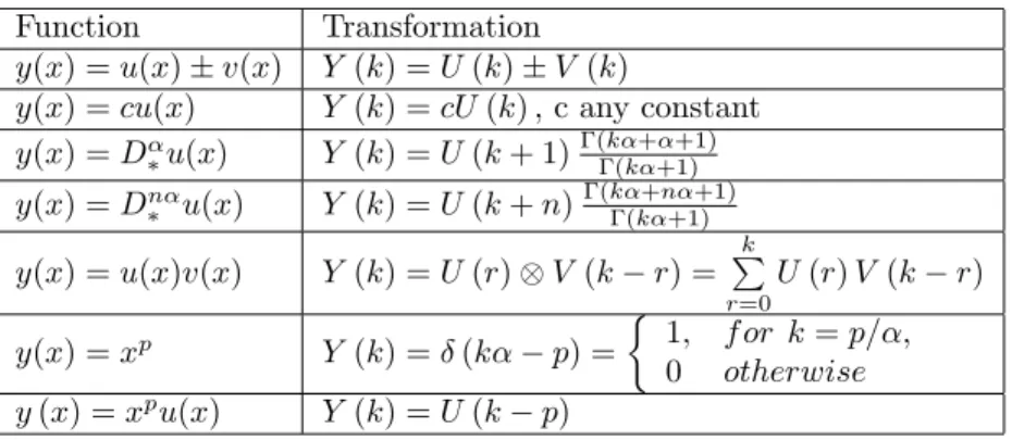
Equation (2.3) implies that the concept of fractional di¤erential transformation is derived from the fractional power series expansion. From de…nitions of (2.3) and (2.4), some basic properties of the fractional di¤erential transformation are summarized in Table 1.

Function Transformation y(x) = u(x) v(x) Y (k) = U (k) V (k)

y(x) = cu(x) Y (k) = cU (k) ; c any constant y(x) = D u(x) Y (k) = U (k + 1) (k + +1)_{(k +1)} y(x) = Dn _{u(x) Y (k) = U (k + n)} (k +n +1) (k +1) y(x) = u(x)v(x) Y (k) = U (r) V (k r) = k P r=0 U (r) V (k r) y(x) = xp _{Y (k) = (k p) =} 1; f or k = p= ; 0 otherwise y (x) = xp_{u(x) Y (k) = U (k p)}

Nonlinear Function Transformed Form N y(x) = y3=2_(x) N (0) = y3=2₀ N (1) =3₂py0y1 N (2) = 3 8 y12 p_y 0 + 3 2 p_y 0y2 N (3) = ₁₆1 y13 y3=20 +3₄y1y2 p_y 0 + 3 2 p_y 0y3 N y(x) = ey(x) N (0) = eY (0) N (1) = Y (1)eY (0) N (2) = Y (2) + 1 2!Y 2_{(1) e}Y (0) N (3) = Y (3) + Y (1)Y (2) + _3!1Y3_{(1) e}Y (0) .. . N y(x) = P1 k=0 xk k! h dk dxkN y(x) i x=0 = P1 k=0 xk k! dk dxkN 1 P r=0 Y (r)xr x=0 MapleCode restart;

NF:=N(y(x): # Nonlinear Function m:=5: #Order y[x]:=sum(y[b]*x^b,b=0..m): NF[x]:=subs(y(x)=y[x],NF): s:=expand(NF[x],x): dt:=unapply(s,x): for i from 0 to m do n[i]:=((D@@i)(dt)(0)/i!): print(N[i],n[i]); #Transform Function

od:

Table 2: The Di¤erential Transformation of Nonlinear Functional and MAPLE codes [15]

It is also given the transform forms of nonlinear functionals [15]. According to this study, transform forms of some of nonlinear functionals and maple code are presented in Table 2.

3. Numerical Application

In this section, we apply fractional di¤erential transform for …nding an approx-imate solution of the Thomas -Fermi equation.

Consider the nonlinear Thomas Fermi equation

(3.1) y00(x) = y

3=2_(x)

p_x with initial condition

(3.2) y(0) = 1; lim

Then, by using the basic properties of the transformation from Table 1 and Table 2, we can …nd the transformed form of equation (3.1) as

(3.3) (k 1) Y (k + 4) k+6 2 k+2 2 = N (k) or (3.4) Y (k + 4) k+6 2 k+2 2 = N (k + 1)

where Y (k) and N (k) are the transformations of the functions y(x) and N y(x) =

y3=2(x)

x1=2 respectively. Using the initial condition (3.2), we have

(3.5) Y (0) = 1; Y (1) = 0; Y (2) = A;

Now, substituting (3.5) into (3.4), we obtain the following Y (k) values succes-sively, Y (3) = 4₃ Y (4) = 0 Y (5) = 2A₅ Y (6) = 1₃ Y (7) = 3A2 70 .. .

Finally, using the inverse transformation of fY (k)g10k=0, we …nd

(3.6) y(x)=

10

P

k=0

Y (k)xk=2= 1 + Ax+4x₃3=2+2Ax₅5=2+x₃3+3A2₇₀x7=2+2Ax₁₅4 + ₂₇2 ₂₅₂A3 x9=2₊A2_x5

175

Setting t = x1=2_{, the approximation of y(t) is readily found to be}

(3.7) y(t) = 10 P k=0 Y (k)tk_{= 1 + At}2₊4t3 3 + 2At5 5 + t6 3 + 3A2_t7 70 + 2At8 15 + ₂₇2 ₂₅₂A3 t9₊A2_t10 175

The aim of this paper is to study the mathematical behavior of the potential y(x) and to determine the initial slope of the potential y0_{(0) It was formally}

shown [6,8] that this goal can be achieved by forming Pade approximants [5] which have the advantage of manipulating the polynomial approximation into a rational function to gain more information about y(x). It is well-known that Pade approximants will converge on the entire real axis [6] if y(x) is free of singu-larities on the real axis. Moreover, it is to be noted that Pade …nding algorithms are built-in utilities in most symbolic languages [6] such as Maple, Matlab and Mathematica. More importantly, the diagonal approximant is the most accurate

approximant, therefore we will construct only the diagonal approximants in the following discussions. Using the boundary condition lim

x!1y(x) = 0, the

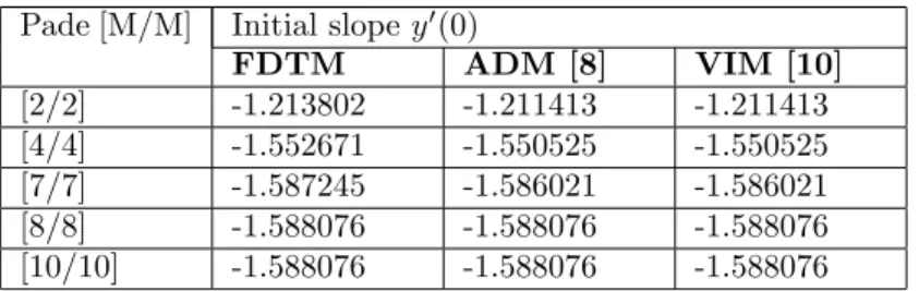
diago-nal approximant [M/M] vanishes if the coe¢ cient of t with the highest power vanishes. Using the Maple built-in utilities to solve the resulting polynomials, the values of the initial slope y0(0) are listed in Table 3. In addition, Table 3 shows the comparison of the values of the initial slope y0_{(0) with fractional}

di¤erential transform method, Adomian decompositon method and variational iteration method. The existing results in literature are compared with the one obtained by Kobayashi [3].

Pade [M/M] Initial slope y0₍₀₎

FDTM ADM [8] VIM [10] [2/2] -1.213802 -1.211413 -1.211413 [4/4] -1.552671 -1.550525 -1.550525 [7/7] -1.587245 -1.586021 -1.586021 [8/8] -1.588076 -1.588076 -1.588076 [10/10] -1.588076 -1.588076 -1.588076

Table 3: Comparison of the FDTM with di¤erent techniques for initial slope y0₍₀₎

4. Concluding remarks

In this study, using FDTM, it is obtained, for the …rst time, the solutions of nonlinear di¤erential equations which consists of in…nite boundary value. This method applied to the Thomas-Fermi equation. The approximate solution of the problem can be obtained to any desired order of the suggested method. The numerical scheme gives almost analytical solution depending on the type of the transformation method. It is also showed that the numerical algorithm of this method is easy to compute the necessary coe¢ cients or to set a computer code in order to get as many terms of the series solution as we need.

References

1. L. H. Thomas, The calculation of atomic …elds, Proc. Cambridge Phil. Soc. 23, (1927), 542.

2. E. Fermi, Un metodo statistico per la determinazione di alcune priorietA dell’atome, Rend. Accad. Naz. Lincei 6(6), (1927), 602.

3. S. Kobayashi,T. Matsukuma, S. Nagai, K.Umeda, Some coe¢ cients of the TFD function, J. Phys. Soc. Japan 10, 1955, 759-765.

4. E. Hille, On The Thomas-Fermi Equation, Proc Natl Acad Sci 62 (1), 1969, 7–10. 5. G.A. Baker, Essentials of Pade eapproximants, Academic Press, London, 1975. 6. J. Boyd, Pade approximant algorithm for solving nonlinear ordinary di¤erential equation boundary value problems on an unbounded domain, Comput. Phys. 11 (3), 1997, 299-303.

7. G. Adomian, Solution of the Thomas-Fermi Equation, Applied Mathematics Letters 11 (3), 1998, 131-133.

8. A.M. Wazwaz, The modi…ed decomposition method and Pade approximants for solving Thomas -Fermi equation, Applied Mathematics and Computation 105, 1999, 11-19.

9. J.H. He, Variational approach to the Thomas-Fermi equation, Applied Mathematics and Computation 143, 2003, 533-535.

10. M.A. Noor, S.T. Mohyud-Din, M. Tahir, Modi…ed Variational Iteration Methods for Thomas-Fermi Equation, World Applied Sciences Journal 4(4), 2008, 479-486. 11. B. Yao, A series solution to the Thomas–Fermi equation, Applied Mathematics and Computation 203, 2008, 396–401.

12. H. Khan, H. Xu, Series solution to the Thomas–Fermi equation, Physics Letters A 365, 2007, 111–115.

13. J. K. Zhou, Di¤erential Transformation and its Applications for Electrical Circuits, Huarjung University Press, China, 1986.

14. G. Oturanc, A. Kurnaz, Y. Keskin, A new analytical approximate method for the solution of fractional di¤erential equations, International Journal of Computer Mathematics 85(1), 2008,131–142.

15. Y. Keskin, G. Oturanç, The di¤erential transform methods for nonlinear functions and its applications, Selçuk Journal of Applied Mathematics 9(1), 2008, 69-76. 16.A. Kurnaz, G. Oturanç, The di¤erentialtransformapproximation for thesystem ofor-dinary di¤erential equations. International Journal of Computer Mathematics 82, 2005, 709–719.

17. Z.M. Odibat, N.T. Shawagfeh, Generalized Taylor’s formula. Applied Mathematics and Computation 186, 2006, 286–293.

18. R. Goren‡o, F. Mainardi, Fractional calculus: integral and di¤erential equations of fractional order. Fractals and Fractional Calculus in Continuum Mechanics, Springer, 1997.

19. K. Diethelm, N.J. Ford, A.D. Freed, Y. Luchko, Algorithms for the fractional calculus: a selection of numerical methods, Computer Methods in Applied Mechanics and Engineering 194, 2005, 743–773.

20. I.H. Abdel-Halim Hassan, Di¤erent applications for the di¤erential transformation in the di¤erential equations, Applied Mathematics and Computation 129, 2002, 183– 201.

21. S. Momani,V.S. Erturk, Solutions of non-linear oscillators by the modi…ed di¤eren-tial transform method,Computers and Mathematics with Applications 55 (2008),833– 842.