The effect of demand uncertainty on the decisions and revenues in the two-class revenue management model

Tam metin

(1)İktisat İşletme ve Finans 30 (347) 2015 : 95-120 www.iif.com.tr doi: 10.3848/iif.2015.347.3789. se. 7:2 1 4:1. 6/2. 01. 51. Received 26 November 2012; received in revised form 9 October 2013; accepted 16 January 2014. +0 30 0. Ayşe Kocabıyıkoğlu (a). 5/0. :0. rih. Ta. 6],. 11. .2.. IP i],. il. :[ 13. 9.1. 79. ge. Abstract. We explore the impact of changes in market conditions on optimal allocation decisions and revenues, within the standard two-class revenue management framework, using stochastic dominance relations. We show that an increase in market size leads to higher revenues, and the number of units allocated to the high-end class increases in its market size. The direction of the change in optimal allocation and revenues in response to changes in the variability of the high-end market depends on the relationship between the high and lowend prices. Our structural and numerical results suggest higher variability in the market is generally detrimental to revenues. Keywords: Revenue Management, Production Management. JEL Classification: M11.. İnd. ire. n:. [B. ilk. en. tÜ niv. er. sit. es. Özet. Talep Belirsizliğinin İki Sınıflı Gelir Yönetimi Modellerinin Karar ve Gelirleri Üzerindeki Etkisi Bu makalede talep belirsizliğinin standart iki sınıflı gelir yönetimi modelini üzerindeki etkisi analitik ve sayısal olarak incelenmektedir. Talep belirsizliğinin bu modelden elde edilen optimal tahsis kararı, ve iki sınıftan olan ve toplam gelirler üzerindeki etkisi stokastik ilişkiler kullanılarak incelenmektedir. Talebin stokastik olarak büyümesinin elde edilen optimal gelirleri, ve daha değerli alıcı sınıfına ayrılan kapasite miktarını arttırdığı analitik olarak gösterilmektedir. Talebin varyansındaki değişikliklerin toplam gelirler, her iki dınıftan elde edilen gelirler, ve tahsis kararları üzerindeki etkisinin ise iki alıcı sınıfının satış fiyatları arasındaki ilişkiye bağlı olduğu görülmüştür. Makalede sunulan analitik ve sayısal sonuçlar talep varyansındaki olası bir artışın gelirlere etkisinin genellikle olumsuz olduğunu göstermektedir. Anahtar Kelimeler: Gelir Yönetimi, Üretim Yönetimi. JEL Sınıflaması: M11.. B. İndiren: [Bilkent Üniversitesi], IP: [139.179.2.116], Tarih: 05/06/2015 14:17:21 +0300. l. The Effect of Demand Uncertainty on the Decisions and Revenues in the Two Class Revenue Management Model. (a) Faculty of Business Administration, Bilkent University , Bilkent, Ankara, Turkey E-mail: aysekoca@bilkent.edu.tr 2015© Her hakkı saklıdır. All rights reserved..

(2) İktisat İşletme ve Finans 30 (347) Şubat / February 2015. .2.. 11. 6],. Ta. rih. :0. 5/0. 6/2. +0 30 0. 7:2 1. 4:1. 01. 51. se. er. sit. es. i],. IP. :[ 13. 9.1. 79. ge ire. n:. [B. ilk. en. tÜ niv. il. 96. İnd. B. İndiren: [Bilkent Üniversitesi], IP: [139.179.2.116], Tarih: 05/06/2015 14:17:21 +0300. l. 1. Introduction In this paper, we study the impact of changing market conditions on the firm’s allocation decision and revenues within the standard two-class revenue management framework. In this model, a firm sells a fixed resource/capacity (such as seats on a flight or rooms in a hotel) to two market segments with sequential price levels and uncertain demands. The customers with higher willingness to pay arrive later in the sales horizon, and the firm determines the protection level, i.e. the number of units to protect for the high-end class, with the objective of maximizing revenues. We focus on this model, because it is the base model for revenue management and the oldest revenue management model still in use. Market factors have been acknowledged as the major source of uncertainty in many operations management models (Davis 1993), and have considerable impact on how operational processes are managed and their results. Hence, it is worthwhile to study how revenue management systems behave under changing market conditions. We first investigate the impact of a change in the market size (modeled with a change in the demand distribution in the sense of first order stochastic dominance, see Section 3 for a formal definition) on optimal allocation and revenues. Throughout the paper, “optimal” refers to the expected revenue maximizing level. We show that it is more profitable for the firm to allocate a greater portion of the fixed resource to the customers with higher willingness to pay (henceforth referred to as class 1), i.e., increase the protection level, when the size of its market increases; a stochastically bigger class 1 market also leads to higher class 1 and total revenues if the protection level is chosen optimally. A change in the size of the low-end market (henceforth referred to as class 2), on the other hand, results in an increase in the revenues obtained from this class, while its impact on the optimal class 1 and total revenues is not clearly determined. Our numerical experiments suggest that although a larger class 2 market generally leads to lower revenues from the high-end market, this relationship is reversed when (1) the values of class 1 and class 2 sales are close, (2) class 2 market is stochastically large, and (3) there is ample capacity. We also observe that total revenues increase in the size of the class 2 market, leading us to conclude that larger markets generally have a positive impact on revenues. Our analysis of changes in market variability (modeled with a mean preserving spread, formalized in Section 4) shows that an increase in the highend market variability always leads to lower revenues given an allocation; however, the behavior of the firm’s revenues when the protection level is chosen optimally is not clearly determined. In particular, when the ratio of the class 2 price to the class 1 price is greater than ½ (and hence, the values of class.

(3) İktisat İşletme ve Finans 30 (347) Şubat / February 2015. +0 30 0. 7:2 1. 4:1. rih. :0. 5/0. 6/2. 01. 51. se. ge IP. i],. es. sit. er. İnd. ire. n:. [B. ilk. en. tÜ niv. il. :[ 13. 9.1. 79. .2.. 11. 6],. Ta. Literature Review. The literature on revenue management is vast; the most comprehensive works to date are the books by Talluri and van Ryzin (2004) and Phillips (2005). McGill and van Ryzin (1999) review the earlier revenue management literature, Elmaghraby and Keskinocak (2003) focus on dynamic pricing, and Shen and Su (2007) discuss customer behavior modeling. Papers most closely related to the model considered in this work are those that study the allocation of a single resource among different customer segments when demand classes arrive sequentially - see e.g. Littlewood (1972), Belobaba (1989), Curry (1990), Wollmer (1992), Brumelle and McGill (1993), Robinson (1995). There are few papers in the operations management literature that study the impact of stochastically changing demand conditions on an operational model. In the newsvendor context, Gerchak and Mossman (1992) study the magnitude of change in optimal cost and order quantity when there is an increase in demand variability. They show that higher variability leads to higher costs. Song (1994) focuses on the impact of changing leadtime variability on optimal inventory decisions. Ridder et al. (1998) study the behavior of optimal cost with respect to changing market risk under different variability orders. Li and Atkins (2005) focus on the impact of changing demand variability within the price-setting newsvendor problem, and characterize the direction of the change on optimal price and order quantity. Song and Zipkin (1996) consider a more general inventory system than the newsvendor, and study. B. İndiren: [Bilkent Üniversitesi], IP: [139.179.2.116], Tarih: 05/06/2015 14:17:21 +0300. l. 1 and class 2 sales to the firm are close), optimal class 2 revenues increase as the class 1 market gets more variable, while the optimal protection level, class 1 and total revenues move in the opposite direction. When the price ratio is less than ½, on the other hand, the optimal protection level decreases, and revenues from class 2 sales increase as class 1 market variability increases, while class 1 revenues may increase (because of the increase in the optimal protection level) or decrease (because of higher variability). Our numerical experiments suggest that the protection level effect dominates, leading to higher revenues from class 1 sales, when class 1 sales are more valuable compared to class 2 sales, or when class 2 market variability is low. We also investigate the impact of a change in the variability of the class 2 market on optimal revenues. We show that a more variable class 2 market leads to lower revenues from this class. Furthermore, although the relationship between class 2 market variability and optimal class 1 revenues is not clearly determined structurally, we observe via our numerical experiments that total and class 1 revenues generally decrease in response to increasing class 2 market variability, leading us to conclude that higher variability is generally detrimental to revenues.. 97.

(4) İktisat İşletme ve Finans 30 (347) Şubat / February 2015. +0 30 0. 7:2 1. 4:1. rih. :0. 5/0. 6/2. 01. 51. se Ta. 6],. ge IP. i],. il. :[ 13. 9.1. 79. .2.. 11. Structure. The rest of the paper is organized as follows. Our model, assumptions and notation are presented in Section 2. Section 3 provides structural results and numerical experiments that provide insights regarding the impact of changing market size on optimal allocation decisions and revenues. Similar analysis on changes in market variability is presented in Section 4. Section 5 concludes the paper.. 98. İnd. ire. n:. [B. ilk. en. tÜ niv. er. sit. es. 2. The Model This section sets up our basic model, main assumptions and notation. In the standard two-class revenue management model, the firm determines the allocation of a fixed resource, denoted by C, between two market segments (class 1 and class 2) with sequential price levels ( p1 and p2 with p1 > p2 without loss of generality), with the objective of maximizing revenues. In typical revenue management settings, fixed costs are high and variable costs are negligible; hence, earnings are stated in terms of revenues. The firm sets the number of units reserved for the higher priced class, called the protection level, denoted by x. The firm faces uncertain demands D1 and D2 from the higher priced class (class 1), and the lower priced class (class 2), respectively; class 2 customers arrive before class 1 customers. The allocation decision is made. B. İndiren: [Bilkent Üniversitesi], IP: [139.179.2.116], Tarih: 05/06/2015 14:17:21 +0300. l. how increased lead time variability affects the inventory size via numerical experiments; while Song et al. (2010) consider the impact of stochastically larger and more variable lead time on cost and policy parameters. Federgruen and Wang (2012) study when the optimal policy and cost parameters are monotone in demand uncertainty for a similar system. Gupta and Cooper (2005) study stochastic orderings of yield rates that guarantee a coherent ordering of profits. Li and Zheng (2006) compare optimal policies under certain and uncertain yield rates, and show that uncertainty leads to higher prices and lower expected profits. In the revenue management context, Cooper and Gupta (2006) focus on how simultaneous changes in demand under various stochastic orders impact optimal revenues. Araman and Popescu (2010) show stochastically larger or less variable audiences do not necessarily command lower capacity allocations in the media broadcasting advertising market. Akcay et al. (2009) consider a multi-period revenue management problem where a firm sells a fixed inventory to multiple customer classes, and study the impact of varying problem parameters, including an increase in the arrival probability. Their model can incorporate a set up similar to ours if arrival probabilities are chosen such that customer classes with lower valuations arrive earlier in the sales horizon..

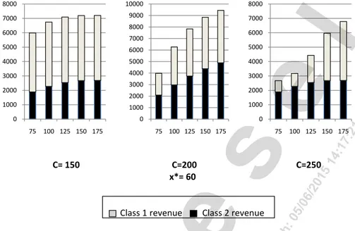
(5) İktisat İşletme ve Finans 30 (347) Şubat / February 2015. before demand from either class is realized. Letting r1 ( x) and r2 ( x) denote the revenue obtained from class 1, and class 2, respectively, for a given protection level x, the firm’s problem is formally modeled as,. +0 30 0. 7:2 1. 4:1. 5/0. 6/2. 01. 51. se. Sales to class 2, min( D2 , C − x) , is constrained by the demand for this class, and the booking limit, C-x, i.e., the units available for sale to class 2. Similarly, to class 1 is the minimum of the demand and available units maxsales x R ( x ) = r1 ( x ) + r2 ( x ) = p1 E [ min( D1 , max(C − D2 , x ) ] + p2 E [ min( D2 , C − x ) ] . for this class, which may exceed the protection level if class 2 demand falls short of the booking limit. Over-allocating to class 1 leaves the firm with unused capacity, which brings no revenue. Under-allocating to class 1, on the other hand, results in lost class 1 sales; in this case, units that could have been sold to class 1 customers were sold to class 2 customers earlier in the 1 P( D1 ≤ u ) denote the sales horizon at a lower price. Letting P( D1 ≥ u ) =− survival function of D1 , the unique optimal protection level is established by Littlewood (1972). (0.1). :0. ge. P( D1 ≥ x* ) = p2 / p1. 6],. Ta. rih. Proposition 1. (Littlewood, 1972) The revenue function R(x) is quasi-concave in x, and the optimal protection level, x* is given by (0.1). .2.. 11. P( D1 ≥ x* ) = p2 / p1. IP. i],. es. sit. er. tÜ niv. il. :[ 13. 9.1. 79. From (1.1), the optimal protection level is a function of the ratio of class 2 price to class 1 price ( p2 / p1 ), and the distribution of class 1 demand D1 . Intuitively, the expected revenue loss from over- and under-allocating to class 1 is matched at the optimal protection level. When the decision maker overallocates to class 1, she is left with unused capacity that could have been sold to a class 2 customer earlier in the sales horizon and brought p2 , if it had not Figure 1. Optimal revenues under varying price ratios with respect to expected class 2 demand been reserved for class 1. When the decision maker under-allocates to class 12000p1 P ( D1 ≥ x ) , since she16000 8000the other hand, she loses 1, on would have earned p1 from 7000that unit, if it had not been sold to a class 2 customer, 14000 provided there was 10000 ample 12000 6000 demand.. en. Figure 1. Optimal revenues under varying price ratios with respect to expected class 2 demand 8000. B. 10000. ilk. 5000. 16000 3. The Effect of Larger12000 Demand 6000 8000 This section studies the10000 impact of changes in market 7000 14000 6000 size on the firm’s 3000 4000 optimal allocation decision and revenues. We model an increase in the 6000 12000 2000 4000 8000 market size by an increase in D , j=1,2, in the sense of first order stochastic 2000 10000 5000 j 1000 2000 dominance, defined below. Throughout the paper, E[ ] denotes the expectation 6000 8000 4000 0 0 0 operator. 3000 6000 75 100 125 150 175 75 100 125 150 175 75 100 125 150 175. ire. n:. [B. 8000 4000. İnd. İndiren: [Bilkent Üniversitesi], IP: [139.179.2.116], Tarih: 05/06/2015 14:17:21 +0300. l. max x R( x) = r1 ( x) + r2 ( x) = p1 E [ min( D1 , max(C − D2 , x) ] + p2 E [ min( D2 , C − x) ] .. 4000. 2000 1000 0. 4000. p1=120 p2=30 x*= 60 75. 100 125 150 175. 2000 0. p1=120 p2=60 x*= 40 75 100 125 150 175. 2000 0. p1=120 p2=90 99 x*= 20 75 100 125 150 175.

(6) İktisat İşletme ve Finans 30 (347) Şubat / February 2015. +0 30 0. se 5/0. :0. rih. Ta. 6],. 11. .2.. IP. i],. es. sit. il. :[ 13. 9.1. 79. ge. 6/2. 01. 51. 4:1. 7:2 1. 3.1. Larger Class 1 Demand In this section, we investigate the behavior of the optimal protection level and revenues with respect to changes in the size of the high-end market. We show that an increase in its market size leads to more resources being allocated to class 1, and to higher overall revenues. We first study the impact of a change in the size of the class 1 market on the optimal allocation decision. Throughout the paper, we use stochastic dominance relations to compare optimal protection levels and revenues. When D1' SD D1 where SD is any stochastic order, we denote the revenue ' under D as R ' ( x) p1 E  min( D '1 , max(C − D2 , x)  + p2 E [ min( D2 , C − x) ] , = 1 ' ' and the corresponding optimal protection level as x* , i.e. x* = arg max R ' ( x) . For the newsvendor problem, Song (1994) establishes that a stochastically bigger market (modeled by a shift in the sense of FSD) leads to a higher optimal order quantity. The two-class revenue management and the newsvendor problems are structurally close; in both cases, the firm tries to find the quantity to order/allocate that would minimize the instances of turned away customers and unsold units. Hence, we apply Song’s (1994) insight to our problem, and obtain the result below. All proofs are provided in the Appendix.. ire. n:. [B. ilk. en. tÜ niv. er. Proposition 2. The optimal protection level increases in the size of the class ' 1 market, i.e., x* ≥ x* , whenever D1' FSD D1 . This result is quite intuitive; a bigger market size requires more units allocated to the high-end class in order to compensate for the now-higher possibility of turned away customers. Next, we investigate the impact of changing market size on revenues.. B. Remark 1. An increase in the size of the class 1 market leads to higher total revenues, given a protection level x, i.e., R ' ( x) ≥ R( x) whenever D1' FSD D1 . Next, we show that this property is preserved when the protection level is chosen optimally.. 100. İnd. İndiren: [Bilkent Üniversitesi], IP: [139.179.2.116], Tarih: 05/06/2015 14:17:21 +0300. l. Definition 1. A random variable X dominates another random variable Y in the sense of first order stochastic dominance, denoted X FSD Y , if P( X ≥ u ) ≥ P (Y ≥ u ) for all u. This is equivalent to E [ h( X ) ] ≥ E [ h(Y ) ] for all increasing functions h. Remark that, if X FSD Y , then E [ X ] ≥ E [Y ] . Hence, X is stochastically larger than Y . For example, for two distributions X and Y , with X= δ + Y , where δ ≥ 0 , X FSD Y . For more on stochastic orders, the reader is referred to Shaked and Shanthikumar (1994), and Müller and Stoyan (2002)..

(7) D1' FSD D1. İktisat İşletme ve Finans 30 (347) Şubat / February 2015. +0 30 0. 7:2 1. 4:1. 01. 51. se 5/0. :0. rih. Ta. 6],. 11. .2.. ge. 6/2. 3.2. Larger Class 2 Demand This section investigates how the optimal protection level x*, class 2, class 1, and total revenues change when there is a shift in the low-end demand in the sense of the first order stochastic dominance, i.e., when D2' FSD D2 . We show that the optimal class 2 revenue increases in the size of its market, and present numerical insights on the relationship between the size of the class 2 market, and optimal class 1 and total revenues.. IP. i],. es. sit. er. tÜ niv. il. :[ 13. 9.1. 79. 3.2.1. Structural Results First, remark that, from the optimality condition (1), the optimal protection level is determined by the distribution of class 1 demand and the selling prices of the two market segments; hence, the optimal' protection level is not influenced by changes in the class 2 market, i.e., x* = x* , whenever D2' FSD D2 . This, and the fact that class 2 sales, min( D2 , C − x) is decreasing in D2 , leads to the following relationship between the size of the class 2 market and revenues from this class.. İnd. ire. n:. [B. ilk. en. Proposition 4. When there is an increase in the size of the ' class 2 market ( D2' FSD D2), the optimal class 2 revenue increases, i.e., r2 ' ( x* ) ≥ r2 ( x* ) . The impact of a change in the size of the low-end market on the optimal class 1 revenues, on the other hand, is determined by two, typically opposing, effects. Because sales to class 1, min( D1 , max(C − D2 , x) , is restricted by the demand and the number of units available for this class (which might be higher than the protection level x, if class 2 demand falls short of the booking limit), a larger class 2 demand implies less units available to class 1 because there is now a lower possibility of class 2 demand falling short of the booking. B. İndiren: [Bilkent Üniversitesi], IP: [139.179.2.116], Tarih: 05/06/2015 14:17:21 +0300. l. Proposition 3. When there is an increase in the size of the class ' 1 market ( D1' FSD D1 ), (a) the optimal class 1 revenue increases, i.e., r1' ( x* ) ≥ r1 ( x* ) , ' *' (b) the optimal class 2 revenue decreases, i.e., r2 ( x ) ≤ r2 ( x* ) , (c) the optimal *' * total revenue increases, i.e., R ( x ) ≥ R ( x ) . The impact of the changing market size on the optimal class 2 revenues follows from Proposition 2; since class 2 revenue is not a function of the class 1 demand, it is impacted only through the change in the optimal protection level, and class 2 revenues decrease in the number of units allocated to class 1. The high-end revenue, on the other hand, is affected both by the increase in demand (which leads to higher revenues for a given protection level; see Remark 1) and the change in the protection level (which increases; see Proposition 2); these two effects lead to higher revenues from class 1 under the optimal allocation. The increase in optimal class 1 revenues offsets the decrease in the class 2 revenues, resulting in higher total revenues.. 101.

(8) İktisat İşletme ve Finans 30 (347) Şubat / February 2015. +0 30 0. 7:2 1. 4:1. 5/0. :0. rih. Ta. 6],. 11. .2.. IP. il. :[ 13. 9.1. 79. ge. 6/2. 01. 51. se. 3.2.2. Numerical Experiments In this section, we evaluate class 2, class 1 and total revenues under the optimal allocation in response to changing class 2 market sizes with respect to problem parameters such as price, capacity and class 1 demand. We observe that, as proved in the previous section, optimal class 2 revenues increase in the size of its market. The direction of the change in revenues from class 1, on the other hand, depends on the problem environment; in particular, we observe D1  Uniform that, optimal class 1 revenues increase in the size of the class 2 market when: (1) class 1 sales are much more valuable for the firm compared to class 2 sales, (2) there is ample capacity, and (3) class 1 market is stochastically large. We also observe that total revenues increase in response to increases in the D1  Uniform size of the low-end market. We present numerical results for specific problem parameters; extensive numerical experiments with a wide range of parameters suggest that the insights illustrated in this section are robust. ThroughoutDthis 2 � section, class 2 demand (distributed Uniform) is varied consistent with a first order stochastic shift; in particular, we use the following distributions: D2  Uniform Uniform(0,150), Uniform(25,175), Uniform(50,200), Uniform(75,225), and Uniform(100,250), corresponding to expected classD22 � demands of 75, 100, 125, 150 and 175 respectively ( E [ D2 ] =(a+b)/2 for D2  Uniform(a,b)). Uniform. 102. İnd. ire. n:. [B. ilk. en. tÜ niv. er. sit. es. i],. Results with respect to selling prices. Figure 1 presents the optimal class 2, class 1 and total revenues under changing class 2 demands. We kept the class 1 price at p1 =120, and varied the class 2 price to obtain price ratios p2 / p1 = {0.25, 0.5, 0.75}. We chose these values because, when p2 / p1 < 1/ 2 , the 1 � value of class 1 sales to the firm is much higher than theDclass 2 sales, compared to when p2 / p1 > 1/ 2 . Class 1 demand is distributed D1  Uniform(0,80) with Uniform capacity set at C=150. These particular demand and capacity parameters were chosen because revenue management is most relevant when the capacity is binding, yet ample enough to serve both segments. Also remark that, from the optimality condition (1), when class 1 demand is distributed Uniform(a,b), the optimal protection level solves b − ( p2 / p1 )(b − a ) . We observe that the revenues from class 2 increase in the size of its market, as proved in Proposition 4. The direction of the change in optimal D2  Uniform. B. İndiren: [Bilkent Üniversitesi], IP: [139.179.2.116], Tarih: 05/06/2015 14:17:21 +0300. l. limit. This leads to a decrease in revenues obtained from class 1. However, an increase in the size of the class 2 demand also decreases the possibility of being left with unsold units because overall demand is now larger, which leads to higher revenues. The direction of the change in optimal class 1 revenues is determined by the stronger effect. This is further explored with our numerical experiments, presented in the next section..

(9) D1  Uniform. İktisat İşletme ve Finans 30 (347) Şubat / D February 2015  Uniform 1. +0 30 0. 7:2 1. 4:1. rih. :0. 5/0. 6/2. 01. 51. se Ta. 6],. ge IP. i],. es. sit. er. D2  Uniform. İnd. ire. n:. [B. ilk. en. tÜ niv. il. :[ 13. 9.1. 79. .2.. 11. Results with respect to available capacity. In this section, we vary the capacity available, which essentially determines the level of congestion in the system. Figure 2 presents class 2, class 1 and total revenues under the optimal protection level, for varying sizes of class 2 demand, when capacity is equal D1 �2 prices are p =120 and to C=150, C=200, and C=250. The class 1 and class 1 Uniform p2 =30, and the class 1 demand is distributed D1  Uniform(0,80). Remark that, from the optimality condition (1), the number of units available for sale does not impact the optimal protection level, x; hence, it is the same (60) for all capacity levels.. B. İndiren: [Bilkent Üniversitesi], IP: [139.179.2.116], Tarih: 05/06/2015 14:17:21 +0300. l. class 1 revenues, however, depends on the problem environment. As argued above, an increase in the size of the class 2 market leads to fewer number of units being available to class 1 (and hence, to lower revenues from this class); however, it also decreases the possibility of unsold units (and hence, D2 class � increases 1 revenues). When the size of the class D2 �2 market is small (e.g., Uniform D  when Uniform(0,150), or Uniform(25,175)), the total expected demand D1 � 2 is less than the available capacity (e.g., when D2  Uniform(0,150) with Uniform D1  Uniform Uniform(0,80), total expected demand is equal to E [ D1 ] + E [ D2 ] = 40+75=115<150=C), and hence, the possibility of being left with unused capacity is higher. Consequently, when there is an increase in the size of the class 2 market, the decrease in the possibility of unsold units dominates the effect of the available units; hence, revenues from class 1 increase. When the size of the class 2 market is larger however, the expected total demand is close to, and possibly greater than, the available capacity; hence, the possibility of being left with unsold units is already small. In this case, the decrease in the number of units available to class 1 dominates. This effect is particularly Uniform D2  more pronounced when the ratio of class 2 price to class 1 price is higher (e.g., p2 / p1 =0.75), because in this case, the optimal protection level is low, and hence the possibility of being left with unused capacity due to over-allocation is smaller for all levels of class 2 demand.. 103.

(10) İktisat İşletme ve Finans 30 (347) Şubat / February 2015 Figure 1. Optimal revenues under varying price ratios with respect to expected class 2 demand 12000. 8000 7000. 16000 14000. 10000. 12000 8000. 5000. 3000. 8000 6000. se. 4000. 4000. 2000. 2000. 0. 75 100 125 150 175. 100 125 150 175. p1=120 p2=90 x*= 20. 51. p1=120 p2=60 x*= 40. Ta. rih. :0. Class 2 revenue. ge. Class 1 revenue. 5/0. 6/2. p1=120 p2=30 x*= 60. 75 100 125 150 175. 01. 75. 0. 7:2 1. 0. 4:1. 1000. +0 30 0. 2000. IP. i],. es. sit. il. :[ 13. 9.1. 79. .2.. 11. 6],. We observe that the optimal class 1 revenues either monotonically increase (when C=200, C=250), or first increase, and then decrease (C=150) as the size of the class 2 market increases. Having more units for sale increases the 1 there is an increase in the size of the possibility of unsold units; hence, when class 2 market, its impact on the number of unsold units is stronger than its impact on the number of units available to class 1. Optimal class 2 revenues increase, as predicted by Proposition 4. We also observe that total revenues increase as the size of the class 2 market increases.. 104. İnd. ire. n:. [B. ilk. en. tÜ niv. er. Results with respect to high-end demand. Finally, we vary the class 1 demand, consistent with a first orderDstochastic shift; in particular, we calculate 1 � class 1, class 2 and total optimal revenues under the optimal allocation when class 1 demand is distributed D1  Uniform Uniform(0,80), Uniform(10,90), and Uniform(20,100), corresponding to expected class 1 demands of E [ D1 ] =40, 50, and 60 respectively. Capacity is kept at C=150. The selling prices are p1 =120 and p2 =90 in Figure 3, and p1 =120 and p2 =30 in Figure 4. We present both cases, because we observe different trends with respect to the change in optimal class 1 revenues in each case.. B. İndiren: [Bilkent Üniversitesi], IP: [139.179.2.116], Tarih: 05/06/2015 14:17:21 +0300. 10000. 6000. 4000. l. 6000. D2  Uniform.

(11) İktisat İşletme ve Finans 30 (347) Şubat / February 2015 Figure 2. Optimal revenues under varying capacity levels with respect to expected class 2 demand 8000. 10000. 8000. 7000. 9000. 7000. 8000. 4000. 5000. 4000. 3000. 4000. 3000. 3000. 1000. 1000. 0. 0. 0. 75 100 125 150 175. 100 125 150 175. 100 125 150 175. C=250. 51. C=200 x*= 60. Ta. rih. :0. Class 2 revenue. ge. Class 1 revenue. 5/0. 6/2. C= 150. 75. 01. 75. +0 30 0. 2000. 2000. 1000. 7:2 1. 2000. l. 5000. se. 6000. IP. i],. es. sit. er. en. tÜ niv. il. :[ 13. 9.1. 79. .2.. 11. 6],. When the ratio of class 2 price to class 1 price is equal to ¼, i.e., class 1 sales are much more valuable compared to class 2 sales, class 1 revenues � increase as the size of the class D 21market gets bigger, when class 1 demand is Uniform D1 class also stochastically large,under e.g.,varying Uniform(20,100). is observed Figure 3. Optimal revenues 1 market sizes withThis respecteffect to expected class 2 because the increase in the sizedemand; of the pclass 1 market propagates the decrease =¾ / p 2 1 in16000 the possibility of unsold16000 units. It also leads to higher total revenues, as class 14000 2 14000 revenue is also increasing in its market size. When the ratio of class 2 price 14000 12000 to12000 class 1 price is ¾, however, class 1 revenues decrease as class 2 market 12000 10000 gets bigger, regardless of the size of the class 1 market. As discussed above, 10000 10000 8000 when the selling prices are 8000 closer, the optimal protection level is lower, which 8000 6000decrease in the number results in lower possibility of unsold units. Hence, the 6000 6000 of units available to class 1 dominates, and class 1 revenues decrease in the Uniform D  4000 2 4000 4000 size of the class 2 market. 2000 2000. ilk. 2000. B 0. 0. 0. ire. n:. [B. 4. The Effect of More Variable Demand 75 100 125 150 175 75 100 125 150 175 75 100 125 150 175 In this section, we consider the impact of changes in market variability E[D1]=50 1]= 40 1]=60 on optimalE[D revenues and allocations. In order to model a E[D change in market x*= 20 x*= 30 x*= 40 variability, we employ the concept of mean preserving spread, introduced by Rothschild and Stiglitz (1970, 1971).. İnd. İndiren: [Bilkent Üniversitesi], IP: [139.179.2.116], Tarih: 05/06/2015 14:17:21 +0300. 6000. 7000. 5000. 4:1. 6000. Class 1 revenue. Class 2 revenue. 105.

(12) Class 1 revenue. Class 2 revenue. İktisat İşletme ve Finans 30 (347) Şubat / February 2015. 16000. 14000. 14000. 14000. 12000. 12000. 12000. 10000. 10000. 8000. 8000. 6000. 6000. 4000. 4000. 2000. 2000. 8000. 4000. 0. 75 100 125 150 175. E[D1]=60 x*= 40. 01. 51. E[D1]=50 x*= 30. 4:1. 75 100 125 150 175. :0. rih. Class 2 revenue. ge. Class 1 revenue. 5/0. 6/2. E[D1]= 40 x*= 20. 7:2 1. 2000. 0 75 100 125 150 175. +0 30 0. 6000. se. 0. 10000. l. 16000. [B. IP. i],. es. sit. er. ilk. en. tÜ niv. il. :[ 13. 9.1. 79. .2.. 11. 6],. Ta. Definition 2. A random variable X differs from another random variable Y by a mean preserving spread ( X MPS Y ), if they have the same finite mean and if there is an interval (a,b) such that X assigns no greater probability than Y to any open subinterval of (a,b), and X assigns no smaller probability than Y to any open interval either to the left or the right of (a,b). Rothschild and Stiglitz (1970) (and2 also Landsberger and Meilijson 1990, Pratt and Machina 1997) show that this is equivalent to E [ h( X ) ] ≥ E [ h(Y ) ] for all convex functions h . Remark that, if X MPS Y , then Var [ X ] ≥ Var [Y ] . Furthermore, two distributions that differ by a mean preserving spread exhibit single crossing property: if X MPS Y , there exists some k such that P( X ≥ u ) ≤ P (Y ≥ u ) for u ≤ k and P( X ≥ u ) ≥ P (Y ≥ u ) for u ≥ k . An example for two distributions that differ by a mean preserving spread is X = δ Y , where δ ≥ 0 , and Y is a random variable with E [Y ] = 0 . In this case X MPS Y .. B 106. ire. n:. 4.1. More Variable Class 1 Demand This section investigates how optimal allocation decision and revenues behave with respect to changes in the variability of the high-end market. We restrict our analysis to symmetric demand distributions; many traditional demand densities, such as the Normal, Uniform (see Silver and Peterson 1985, Tijms 1994) satisfy this property.. İnd. İndiren: [Bilkent Üniversitesi], IP: [139.179.2.116], Tarih: 05/06/2015 14:17:21 +0300. Figure 3. Optimal revenues under varying class 1 market sizes with respect to expected class 2 demand; p2 / p1 =¾.

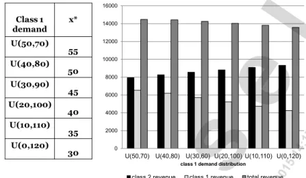
(13) İktisat İşletme ve Finans 30 (347) Şubat / February 2015. 8000. 10000. 9000. 7000. 9000. 8000. 8000. 7000. 7000. 6000. 6000. 4000 2000. 2000 0. 0. 75 100 125 150 175. E[D1]= 40 x*= 60. E[D1]=50 x*= 70. 100 125 150 175. 01. E[D1]=60 x*= 80. Class 2 revenue. ge. Class 1 revenue. 75. 51. 100 125 150 175. 6/2. 75. 7:2 1. 1000. 1000. 0. 4:1. 1000. +0 30 0. 3000. 3000. 2000. 5/0. 4000. rih. 3000. 5000. se. 5000. Ta. 4000. 79. .2.. 11. 6],. 4.1.1. Structural Results For the two class revenue management model, Kocabıyıkoğlu and Göğüş (2012) establish the relationship between the optimal protection level and high-end demand variability. We present their results below, for completeness.. 9.1. Figure 5. Optimal revenues under varying degrees of class 1 market variability; p2 / p1 = 3 / 4. IP. i],. es. sit. er. İnd. ire. n:. [B. ilk. en. tÜ niv. il. :[ 13. Proposition 5. (Kocabıyıkoğlu and Göğüş, 2012) When there is an increase in the variability of the class 16000 1 market, (a) the optimal protection level decreases Class 1 x* 14000 ≥ 1/ 2 if p2 / pdemand , and (b) the optimal protection level increases if p2 / p1 ≤ 1/ 2 . 1 p / p ≤ 1/ 2 When , class 1 sales are much more valuable compared 2 1 12000 U(50,70) to the class 2 sales 55 than when p2 / p1 ≥ 1/ 2 ; hence, over-allocating to 10000 class 1U(40,80) (i.e. being left with unused capacity) is more detrimental to the firm 50 8000 when p2 / p1 ≥ 1/ 2 , whereas under-allocating is more detrimental when U(30,90) p2 / p1 ≤ 1/ 2 . Consequently, p2 / p1 ≥ 1/ 2 , in order to avoid being when 45 6000 left with unused capacity, which has now a higher probability because of U(20,100) 4000 40 the shift of the probability mass from the center to the lower tail of the class U(10,110) 2000 1 distribution, the 35 firm shifts allocation from class 1 to class 2 customers, resulting in lower protection0 levels. When p2 / p1 ≤ 1/ 2 , optimal protection U(0,120) U(50,70) U(40,80)toU(30,60) U(10,110) U(0,120) level increases, in 30 order to avoid selling class U(20,100) 2 customers in the expense class 1 demand distribution of the class 1 customers. Note that, in both cases the optimal protection level class 2 revenue class 1 revenue total revenue moves away from the mean (see the proof of Proposition 5 in the Appendix).. B. İndiren: [Bilkent Üniversitesi], IP: [139.179.2.116], Tarih: 05/06/2015 14:17:21 +0300. 5000. :0. 6000. l. Figure 4. Optimal revenues under varying class 1 market sizes with respect to expected class 2 demand; p2 / p1 = ¼. Note: p1=120, p2=90, D2~Uniform(50,200), C=150.. 107.

(14) İktisat İşletme ve Finans 30 (347) Şubat / February 2015. +0 30 0. 7:2 1. 4:1. 5/0. :0. rih. Ta. 6],. 11. .2.. 9.1. 79. ge. 6/2. 01. 51. se. Proposition 6. Suppose p2 / p1 ≥ 1/ 2 . When there is an increase in the variability of the class 1 market ( D1' MPS D1 ) (a) the optimal class 1 revenue ' *' decreases, i.e., r1 ( x ) ≤ r1 ( x* ) , (b) the optimal class 2 revenue increases, i.e., *' ' *' * r2 ( x ) ≥ r2 ( x ) , and (c) the optimal total revenue decreases, i.e. R ( x ) ≤ R ( x* ) . Low-end revenue is influenced by changes in class 1 demand only through the change in the optimal protection level, which is decreasing in the variability of the class 1 market if p2 / p1 ≥ 1/ 2 by Proposition 5(a). Lower protection levels lead to more available units for class 2, and consequently to higher revenues from this class. Class 1 revenues under the optimal allocation decrease because of increasing demand variability (Remark 2) and the decrease in the optimal protection level (Proposition 5a). The decrease in class 1 revenues dominates the increase in class 2 revenues, resulting in lower total revenues. The impact a change in the variability of class 1 market on optimal revenues when p2 / p1 ≤ 1/ 2 , however, is not clearly determined. The optimal class 2 revenues decrease, because it is affected only through the change in the optimal protection level, which is higher under more variable demand (Proposition 5b).. n:. IP. i],. es. sit. er. [B. ilk. en. tÜ niv. il. :[ 13. Proposition 7. Suppose p2 / p1 ≤ 1/ 2 . When there is an increase in variability of the' class 1 market ( D1' MPS D1 ), the optimal class 2 revenue decreases, i.e., r2 ' ( x* ) ≤ r2 ( x* ) . The optimal class 1 and total revenues may increase or decrease in response to changing class 1 market variability, when p2 / p1 ≤ 1/ 2 . An increase in the variability of the class 1 market leads to lower revenues (Remark 2), but it also leads to more units being allocated to class 1 (Proposition 5b), and hence to higher revenues. With our numerical experiments, presented in the next section, we provide further insights on the relationship between changing market variability and optimal revenues.. B 108. ire. 4.1.2. Numerical Experiments In this section, we first provide an example that illustrates the structural results obtained in Proposition 6. In particular, we evaluate class 1, class 2 and total revenues under varying degrees of class 1 market variability when p2 / p1 ≥ 1/ 2 . Then, we present the results of numerical experiments that. İnd. İndiren: [Bilkent Üniversitesi], IP: [139.179.2.116], Tarih: 05/06/2015 14:17:21 +0300. l. Remark 2. An increase in the variability of the class 1 market leads to lower ' total revenues, given an allocation level x, i.e., R ( x* ) ≤ R ( x* ) whenever D1' MPS D1 . We establish that the above result is preserved when the protection level is chosen optimally, if p2 / p1 ≥ 1/ 2 , with Proposition 6, below..

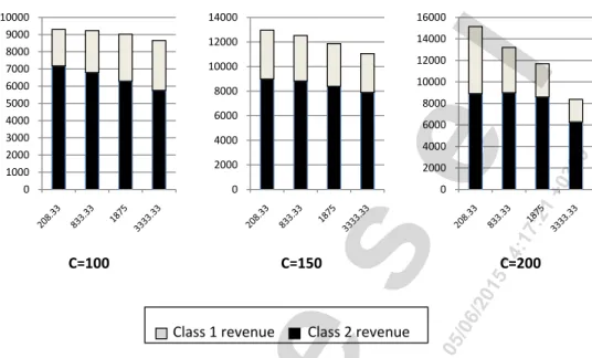
(15) İktisat İşletme ve Finans 30 (347) Şubat / February 2015. +0 30 0. 7:2 1. 4:1. se 5/0. :0. rih. Ta. 6],. 11. .2.. IP. i],. es. sit. il. :[ 13. 9.1. 79. ge. 6/2. 01. 51. Example for Proposition 6. Figure 5 plots the optimal class 1, class 2 and D2under � total revenues varying degrees of class 1 demand variability, and price p1 3 / 4 > 1/ 2 ). Class 2 demand is levels p1 =120 and p2 =90 (i.e., p2 /= distributed with capacity C=150. Remark that, the Uniform D2  Uniform(50,200), D2  Uniform optimal protection level decreases as the class 1 market gets more variable. D '1 � to class 1 leads to higher class 2 This decrease in D1the � number of units allocated revenues (Proposition 6b). For example, when the class 1 demand distribution changes from D1  Uniform Uniform(40,80) to D1  Uniform Uniform(30,90) (hence leading ' = 8543class > 8250 r2 (50) to higher variability), this change impacts rthe optimal 2 =revenues 2 (45) through the change in the protection level (which decreases from 50 to 45). The corresponding class 2 revenue levels are r2 ' (45) = 8543 > 8250 = r2 (50).  Uniform The optimal class 1 revenues, on the other hand, are affected by bothD1the decrease in the protection level (which leads to a decrease in revenues of r1 (50) − r1 (45) = 6183 − 5866 = 317 ) and the increase in variability (which leads to a decrease in revenues of r1 (45) − r '1 (45) = 5866 − 5713 = 153 ); resulting in an overall decrease of 470. D2  Uniform D2  Uniform. İnd. ire. n:. [B. ilk. en. tÜ niv. er. D2 � Results with respect to selling prices when p2 / p1 ≤ 1/ 2 . In this section, we keep the class 1 price at p1 =120, and vary the class 2 price to obtain price ratios p2 / p1 ={0.125, 0.25, 0.375}. Class 2 demand is distributed D2  Uniform Uniform(50,200), with capacity C=150. Figure 6 presents class 1, class 2 and total revenues under the optimal allocation (the optimal protection levels for each demand and price ratio pair are given in Table 1 in the Appendix).. B. İndiren: [Bilkent Üniversitesi], IP: [139.179.2.116], Tarih: 05/06/2015 14:17:21 +0300. l. evaluate revenues under changing class 1 market variability with respect to several problem parameters. In our numerical experiments, we focus on examples where p2 / p1 ≤ 1/ 2 , because, as discussed above, the relationship between the variability of the class 1 market and optimal revenues is not clearly determined in this case. We observe that optimal class 1 and total revenues generally decrease in the face of increasing class 1 variability. Throughout this section, class 1 demand is varied in a manner consistent with D1 � a mean preserving spread. In particular, the high-end demand is distributed D1  Uniform D1  Uniform Uniform(50,70), Uniform(40,80), Uniform(30,90), Uniform(20,100), Uniform(10,110), Uniform(0,120), corresponding to expected class 1 demand E [ D1 ] = 60 and demand variances of 33.33, 133.33, 300, 533.33, 833.33 and 1200, respectively.. 109.

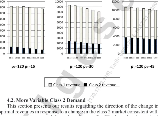
(16) Class 1 revenue. Class 2 revenue. İktisat İşletme ve Finans 30 (347) Şubat / February 2015 Figure 5. Optimal revenues under varying degrees of class 1 market variability; p2 / p1 = 3 / 4 16000. U(10,110) U(0,120). 50. l. 8000. 45. 6000. 40. 4000. 35. 2000. 30. 0. +0 30 0. 10000. 7:2 1. U(20,100). 12000. 55. 4:1. U(30,90). 14000. U(50,70) U(40,80) U(30,60) U(20,100) U(10,110) U(0,120). 51. U(40,80). 01. class 1 demand distribution. total revenue. 6/2. class 1 revenue. 5/0. class 2 revenue. :0. ge. Note: p1=120, p2=90, D2~Uniform(50,200), C=150.. IP. i],. il. :[ 13. 9.1. 79. .2.. 11. 6],. Ta. rih. We observe that the optimal class 2 revenue decreases as the class 1 market gets more variable, as proved in Proposition 7. The optimal class 1 revenue first increases, and then decreases in response to increasing variability in its market; the increasing trend lasts longer when the ratio of class 2 price to class 1 price is small (e.g., when p2 / p1 =0.125). This is observed because in Uniform this case, classD11 sales are much more 3valuable for the firm than class 2 sales and hence the increase in the number of units available to class 1 dominates the decrease in revenues due to higher demand variability. Total revenues exhibit a similar trend.. 110. İnd. ire. n:. [B. ilk. en. tÜ niv. er. sit. es. Results with respect D2 � to low-end demand when p2 / p1 ≤ 1/ 2 . In this section, D1  Uniform we vary the class 2 demand consistent with a mean preserving spread. In particular, we evaluate class 1, class 2 and total revenues when class 2 demand is distributed D2  Uniform Uniform(100,150), Uniform(50,200) and Uniform(0,250), D1 of  Uniform corresponding to expected class 2 demand E [ D2 ] =125, and variances 208.33, 1875, and 5208.33, respectively. Capacity is set at C=150, and class 1 and class 2 selling prices are p1=120 and p2=30. Figure 7 presents our results (the optimal protection D levels under the demand distributions and price levels 2 � considered are given in Table 1 in the Appendix). When class 2 variability is higher, (e.g., when D2  Uniform Uniform(50,200) and Uniform(0,250)), class 1 D2 � revenues first increase, and then decrease in class 1 market variability, whereas class 1 revenues increase monotonically in the face of increasing variability in its market, when class 2 market variability is low (e.g., when D2  Uniform. B. İndiren: [Bilkent Üniversitesi], IP: [139.179.2.116], Tarih: 05/06/2015 14:17:21 +0300. U(50,70). x*. se. Class 1 demand.

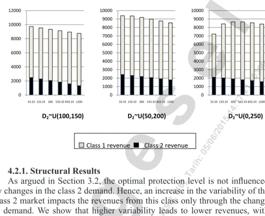
(17) İktisat İşletme ve Finans 30 (347) Şubat / February 2015. 8000. 6000. 5000. 6000. 5000. 4000. 4000. 3000. 4000. 3000. 2000. 2000. 1000. 1000. 2000. 6],. p1=120 p2=45. Class 2 revenue. 9.1. 79. Class 1 revenue. Ta. p1=120 p2=30. 33.33 133.33 300 533.33 833.33 1200. 11. p1=120 p2=15. 0. 33.33 133.33 300 533.33 833.33 1200. rih. 533.33 833.33 1200. .2.. 300. :0. 0. 33.33 133.33. ge. 0. +0 30 0. 7000. 6000. 7:2 1. 10000. 4:1. 8000. 51. 7000. 12000. 01. 9000. 6/2. 10000. 8000. 5/0. 9000. se. Figure 6. Optimal revenues under varying price ratios with respect to class 1 variance. 10000 8000 6000 4000 2000. IP. i],. es. sit. er. ilk. [B. n: ire İnd. 12000. en. tÜ niv. il. :[ 13. 4.2. More Variable Class 2 Demand This section presents our results regarding the direction of the change in optimal revenues in response to a change in the class 2 market consistent with a mean preserving spread, i.e., when D2' MPS D2 . We show that the optimal revenues from class 2 decrease as its market gets more variable. Furthermore, our numerical experiments suggest that higher class 2 variability leads to lower revenues from the high-end market, except when the number of units available for sale is low. Total revenues decrease monotonically in response to an increase in the variability of the low-end market. Figure 7. Optimal revenues under varying class 2 market variability with respect to class 1 variance. B. İndiren: [Bilkent Üniversitesi], IP: [139.179.2.116], Tarih: 05/06/2015 14:17:21 +0300. l. Uniform(0,150)); the low variability of class 2 demand absorbs the negative impact of higher class 1 market variability on revenues. Total revenues, on the other hand, either decrease monotonically, or first increase, then decrease, suggesting higher class 1 variability is generally detrimental to revenues.. 10000. 10000. 9000. 9000. 8000. 8000. 7000. 7000. 6000. 6000. 5000. 5000. 4000. 4000. 3000. 3000. 2000. 2000. 111.

(18) İktisat İşletme ve Finans 30 (347) Şubat / February 2015 Figure 7. Optimal revenues under varying class 2 market variability with respect to class 1 variance. 10000. 9000. 9000. 8000. 8000. 7000. 7000. 6000. 6000. 5000. 5000. 4000. 4000. 3000. 3000. 2000. 2000. 2000. 1000. 0. 1000. 0 33.33 133.33 300 533.33 833.33 1200. +0 30 0. 4000. 7:2 1. 6000. 0. 33.33 133.33 300 533.33 833.33 1200. 33.33 133.33 300 533.33 833.33 1200. D2~U(0,250). 51. D2~U(50,200). rih. :0. 5/0. Class 2 revenue. ge. Class 1 revenue. 6/2. 01. D2~U(100,150). :[ 13. 9.1. 79. .2.. 11. 6],. Ta. 4.2.1. Structural Results As argued in Section 3.2, the optimal protection level is not influenced 4 by changes in the class 2 demand. Hence, an increase in the variability of the class 2 market impacts the revenues from this class only through the change in demand. We show that higher variability leads to lower revenues, with Proposition 8, below.. 112. İnd. ire. n:. [B. ilk. en. IP. i],. es. sit. er. tÜ niv. il. Proposition 8. When there is an increase in the variability of the 'class 2 market ( D2' MPS D2 ), the optimal class 2 revenue decreases, i.e., r2 ' ( x* ) ≤ r2 ( x* ) . The impact of higher class 2 variability on class 1 revenues under the optimal allocation, however, is not clearly determined. As noted above, a change in class 2 demand impacts the number of units available for class 1 ( max(C − D2 , x)), and consequently, class 1 sales. A mean preserving shift in the class 2 demand implies a shift of probability mass from the center to the tails. The shift to the lower tail might result in more units being available to class 1 (and hence, higher revenues), but also in a higher possibility of unsold units (and hence, lower revenues). The shift to the upper tail, on the other hand, leads to higher class 2 demand, and consequently to fewer units being available to class 1 (and lower revenues), and a lower possibility of unsold units (and higher revenues). This tradeoff is further explored in the next section with numerical experiments.. B. İndiren: [Bilkent Üniversitesi], IP: [139.179.2.116], Tarih: 05/06/2015 14:17:21 +0300. 8000. 4:1. 10000. l. 10000. se. 12000.

(19) D1  Uniform. İktisat İşletme ve Finans 30 (347) Şubat / February 2015. +0 30 0. se 5/0. :0. rih. Ta. 6],. 11. .2.. IP. il. :[ 13. 9.1. 79. ge. 6/2. 01. 51. 4:1. 7:2 1. D1 � Results with respect to available capacity. In this section, we evaluate revenues under the optimal allocation for capacity levels C=100, C=150 and C=200. Class 1 demand is distributed D1  Uniform(0,80), and prices are Uniform given by p1 =120 and p2 =90 (implying an optimal protection level of 20). Note that, since class 1 demand remains the same, and the expected class 2 demand does not change when the distribution shifts by a mean preserving spread, lower available capacity implies a busier, more congested system. Figure 8 presents our results. We observe that the optimal class 2 revenues decrease as the variability of its market increases, as predicted by Proposition 8. The optimal class 1 revenues either monotonically increase D(e.g., when C=100), or decrease 2  Uniform (e.g., C=150, C=200). As argued above, increasing variability is generally detrimental to revenues; however, when the number of units available for sale is low, the system absorbs the negative impact of the shift of probability mass from the center to the tails, leading to higher class 1 revenues. Total revenues decrease as class 2 market variability increases.. İnd. ire. n:. [B. ilk. en. tÜ niv. er. sit. es. i],. Results with respect to high-end demand. In this section, we vary the highend demand consistent with a mean preserving spread. In particular, Figure 9 D1 �under the optimal protection level, presents class 2, class 1 and total revenues when class 1 demand is distributed D1  Uniform Uniform(20,60), Uniform(10,70), Uniform(0,80), corresponding to expected class 1 demand E [ D1 ] =40, and variances 133.33, 300, 533.33, respectively. Capacity is set at C=150, and prices are p1 =120 and p1 =90. From Figure 9, class 2, class 1 and total revenues under the optimal allocation decrease as the variability of the class 2 market increases, leading us to conclude that higher variance in the low-end market is generally detrimental to revenues. D2  Uniform. B. İndiren: [Bilkent Üniversitesi], IP: [139.179.2.116], Tarih: 05/06/2015 14:17:21 +0300. l. 4.2.2. Numerical Experiments In this section, we present the results of numerical experiments that evaluate class 2, class 1 and total revenues under varying degrees of class 2 market variability with respect to problem parameters such as capacityDand 2 � class 1 demand. Throughout this section, we consider the following class 2 demand distributions, obtained through mean preserving shifts: D2  Uniform Uniform(75,125), Uniform(50,150), Uniform(25,175), Uniform(0,200), corresponding to variances of 208.33, 833.33, 1875 and 3333.33, respectively. Note that under all four distributions, expected class 2 demand is equal to 100.. 113.

(20) Figure 8. Optimal revenues under varying capacity levels with respect to class 2 variance. 30 (347) Şubat / February 16000 2015 14000 12000. capacity levels with respect 10000to class 2 variance 8000. 16000. 6000. 14000. 4000. l. 12000. 2000. 10000. 0. 8000. 6000. 0. 2000. C=200. 0. Class 1 revenue. Class 2 revenue. C=200. 51. C=150. 11. 6],. Ta. rih. :0. 5/0. Class 2 revenue. ge. Class 1 revenue. 6/2. 01. C=100. +0 30 0. 4000. C=150. 2000. 7:2 1. C=100. se. 6000. 4000. 4:1. 5000 4000 3000 2000 1000 0. 79. 16000. 9.1. 14000. 14000. :[ 13. 12000. 12000. IP. 10000. 10000. 8000. il. .2.. Figure 9. Optimal revenues under varying class 1 market variability with respect to class 2 variance 14000 12000 10000 8000. i],. 8000 Figure 9. Optimal revenues under varying 6000 class 1 market variability with6000 respect to class 2 variance. 2000 12000. 0. 10000. 10000. 0. 10000. 8000. en ilk. İnd. 0. ire. 2000. 6000. [B. D1~U(20,60) x*=20. n:. 4000. 0. 8000. 8000 6000. 4000. D1~U(10,70) x*=25. D1~U(20,60) x*=20. 6000 4000. 2000. 2000. 0. 0. Class 1 revenue. 114. 2000 12000. tÜ niv. 12000. sit. 14000 2000. 4000 14000. er. 4000 14000. es. 6000. 16000 4000. B. İndiren: [Bilkent Üniversitesi], IP: [139.179.2.116], Tarih: 05/06/2015 14:17:21 +0300. İktisat İşletme ve Finans 10000 14000 9000 12000 8000 10000 7000 Figure6000 8. Optimal revenues under varying 8000 5000 10000 14000 6000 4000 9000 3000 12000 4000 8000 2000 10000 2000 7000 1000 6000 0 8000 0. Class 2 revenue. D1~U(10,70) x*=25. 5 Class 1 revenue. D1~U(0,80) x*=30. Class 2 revenue. D1~U(0,80) x*=30.

(21) İktisat İşletme ve Finans 30 (347) Şubat / February 2015. +0 30 0. 7:2 1. 4:1. rih. :0. 5/0. 6/2. 01. 51. se Ta. 6],. 11. .2.. sit. es. i],. IP. :[ 13. 9.1. 79. ge er. n:. [B. ilk. en. tÜ niv. il ire İnd. B. İndiren: [Bilkent Üniversitesi], IP: [139.179.2.116], Tarih: 05/06/2015 14:17:21 +0300. l. 5. Conclusion In this paper, we study the effect of demand uncertainty on optimal decisions and revenues within the two class revenue management model. We first study the impact of changing market size. We show that it is more profitable for the firm to allocate more to the high-end class as its market gets bigger in the sense of first order stochastic dominance; a bigger market also leads to higher overall revenues. While an increase in the size of the low-end market does not impact optimal decisions, it leads to higher revenues from this class, and, as our numerical experiments suggest, higher total revenues, leading us to conclude that bigger markets are consistently more beneficial for the firm in terms of revenues. We also consider changes in market variability; we summarize previous results that show it is more profitable to increase protection levels when the ratio of prices is less than ½, and decrease protection levels when it is greater than ½. Higher class 1 market variability generally leads to lower revenues, except when the variability in the class 2 market is low. An increase in the variability of the class 2 market, on the other hand, does not impact optimal allocations, but, as our numerical experiments suggest, leads to lower total revenues, leading us to conclude that higher variability is detrimental to the firm’s revenues. Many possibilities exist for future work to build on results presented in this paper. It would be of potential interest to study the impact of changing market factors on multiple-class systems, or settings where the firm jointly determines allocation and market prices, as well as an extension of the current work to asymmetric distributions.. 115.

(22) İktisat İşletme ve Finans 30 (347) Şubat / February 2015. .2.. 11. 6],. Ta. rih. :0. 5/0. 6/2. +0 30 0. 7:2 1. 4:1. 01. 51. se. er. sit. es. i],. IP. :[ 13. 9.1. 79. ge ire. n:. [B. ilk. en. tÜ niv. il. 116. İnd. B. İndiren: [Bilkent Üniversitesi], IP: [139.179.2.116], Tarih: 05/06/2015 14:17:21 +0300. l. References [1] Araman, V.F., I. Popescu. 2010. Media Revenue Management with Audience Uncertainty: Balancing Upfront and Spot Market Sales, Manufacturing & Service Operations Management, 12, 190-212. http://dx.doi.org/10.1287/msom.1090.0262 [2] Aydın S., Y. Akçay, F. Karaesmen. 2009. On the Structural Properties of a Discretetime Single Product Revenue Management Problem, Operations Research Letters, 37, 273279. http://dx.doi.org/10.1016/j.orl.2009.03.001 [3] Belobaba, P. 1989. Application of a Probabilistic Decision Model to Airline Seat Inventory Control, Operations Research, 37, 183-197. http://dx.doi.org/10.1287/ opre.37.2.183 [4] Brumelle, S.L., J.I. McGill. 1993. Airline Seat Allocation with Multiple Nested Fare Classes, Operations Research, 41, 127-137. http://dx.doi.org/10.1287/opre.41.1.127 [5] Cooper W.L., D. Gupta. 2006. Stochastic Comparisons in Airline Revenue Management, Manufacturing & Service Operations Management, 8, 221-234. http://dx.doi. org/10.1287/msom.1060.0098 [6] Curry, R.E. 1990. Optimal Airline Seat Allocation with Fare Classes Nested by Origins and Destination, Transportation Science, 24, 193-207.http://dx.doi.org/10.1287/ trsc.24.3.193 [7] Davis, T. 1993. Effective Supply Chain Management, Sloan Management Review, 34, 35-46. [8] Elmaghraby, W., P. Keskinocak. 2003. Dynamic Pricing in the Presence of Inventory Considerations: Research Overview, Current Practices and Future Directions, Management Science, 49, 1287-1309.http://dx.doi.org/10.1287/mnsc.49.10.1287.17315 [9] Federgruen, A., M. Wang. 2012. Monotonicity Properties of a Class of Stochastic Inventory Systems, Annals of Operations Research 2012, 208, 155-186.http://dx.doi. org/10.1007/s10479-012-1125-2 [10] Gerchak, Y., D. Mossman. 1992. On the Effect of Demand Randomness on Inventories and Costs, Operations Research, 40, 804-807.http://dx.doi.org/10.1287/ opre.40.4.804 [11] Gupta, D., W.L. Cooper. 2005. Stochastic Comparisons in Production Yield Management, Operations Research, 53, 377-384.http://dx.doi.org/10.1287/opre.1040.0174 [12] Kocabıyıkoğlu, A., C.I. Göğüş. 2012. Impact of Market Factors on Revenue Management Decisions: An Experimental Study, Working Paper. [13] Landsberger, M., I. Meilijson. 1990. A Tale of Two Tails: An Alternative Characterization of Comparative Risk, Journal of Risk and Uncertainty, 3, 65-82.http:// dx.doi.org/10.1007/BF00213261 [14] Li, Q., D. Atkins. 2005. On the Effect of Demand Randomness on a Price/Quantity Setting Firm, IIE Transactions, 37, 1143-1153.http://dx.doi.org/10.1080/07408170500288182 [15] Li, Q., S. Zheng. 2006. Joint Inventory Replenishment and Pricing Control for Systems with Uncertain Yield and Demand, Operations Research, 54, 4696-4705http:// dx.doi.org/10.1287/opre.1060.0273 [16] Littlewood, K. 1972. Forecasting and Control of Passenger Bookings, AGIFORS Symposium Proc. 12, Nathanya, Israel. [17] McGill, J.I., G.J. van Ryzin. 1999. Revenue Management: Research Overview and Prospects, Transportation Science, 33, 233-256.http://dx.doi.org/10.1287/trsc.33.2.233 [18] Müller A., D. Stoyan. 2002. Comparison Methods for Stochastic Models and Risks, John Wiley&Sons. [19] Phillips, R.L. 2005. Pricing and Revenue Optimization, Stanford Business Books. [20] Pratt, J.W., M.J. Machina. 1997. Increasing Risk: Some Direct Constructions,.

(23) İktisat İşletme ve Finans 30 (347) Şubat / February 2015. +0 30 0. 7:2 1. 4:1. rih. :0. 5/0. 6/2. 01. 51. se Ta. 6],. 11. .2.. sit. es. i],. IP. :[ 13. 9.1. 79. ge er. n:. [B. ilk. en. tÜ niv. il ire İnd. B. İndiren: [Bilkent Üniversitesi], IP: [139.179.2.116], Tarih: 05/06/2015 14:17:21 +0300. l. Journal of Risk and Uncertainty, 14, 103-127.http://dx.doi.org/10.1023/A:1007719626543 [21] Ridder, A., E. Van der Laan, M. Solomon. 1998. How Larger Demand Variability May Lead to Lower Costs in the Newsvendor Problem, Operations Research, 40, 934-936. http://dx.doi.org/10.1287/opre.46.6.934 [22] Robinson L.W. 1995. Optimal and Approximate Control Policies for Airline Booking with Sequential Nonmonotonic Fare Classes, Operations Research, 43, 252-263. http://dx.doi.org/10.1287/opre.43.2.252 [23] Rothschild, M., J.E. Stiglitz. 1970. Increasing Risk I: A Definition, Journal of Economic Theory, 2, 225-243.http://dx.doi.org/10.1016/0022-0531(70)90038-4 [24] Rothschild, M., J.E. Stiglitz. 1971. Increasing Risk: Its Economic Consequences, Journal of Economic Theory, 3, 66-84.http://dx.doi.org/10.1016/0022-0531(71)90034-2 [25] Shaked, M., J. G. Shanthikumar. 1993. Stochastic Orders, Springer. [26] Shen, Z.J.M., X. Su. 2007. Customer Behavior Modeling in Revenue Management and Auctions: A Review and New Research Opportunities, Production and Operations Management, 16, 713-728.http://dx.doi.org/10.1111/j.1937-5956.2007.tb00291.x [27] Silver, E.A., R. Peterson. 1985. Decision Systems for Inventory Management and Production Planning, Wiley, New York. [28] Song, J.S. 1994. The Effect of Leadtime Uncertainty in a Simple Stochastic Inventory Model, Management Science, 40, 603-613.http://dx.doi.org/10.1287/mnsc.40.5.603 [29] Song, J.S., P. H. Zipkin. 1996. The Joint Effect of Leadtime Variance and Lot Size in a Parallel Processing Environment, Management Science, 42, 1352-1363.http://dx.doi. org/10.1287/mnsc.42.9.1352 [30] Song, J.S., H. Zhang, Y. Hou, M. Wang. 2010. The Effect of Lead Time and Demand Uncertainties in (r, q) Inventory Systems, Operations Research, 58, 68-80http:// dx.doi.org/10.1287/opre.1090.0711 [31] Talluri, K., G. van Ryzin. 2004. The Theory and Practice of Revenue Management, Kluwer Academic Publishers.http://dx.doi.org/10.1007/b139000 [32] Tijms, H.C. 1994. Stochastic Models: An Algorithmic Approach. Wiley, New York. [33] Wollmer, R.D. 1992. An Airline Seat Management Model for a Single Leg Route When Lower Fare Classes Book First, Operations Research, 40, 26-37.http://dx.doi. org/10.1287/opre.40.1.26. 117.

(24) İktisat İşletme ve Finans 30 (347) Şubat / February 2015. +0 30 0. 7:2 1. 4:1. 5/0. ge. 6/2. 01. 51. se. Proof of Remark 1. Since class 2 revenue is not a function of the high-end demand, an increase in the size of the class 1 market impacts total revenues for a given protection level x only through the class 1 revenue r1 ( x) . Class 1 revenue = increases in its market size, because h(u ) ED2 [ min(u , max(C − D2 , x) ] is increasing in u (where EY denotes that the expectation is taken over the random variable Y ), and from the definition FSD, ED'  h( D '1 )  ≥ ED1 [ h( D1 ) ] , 1 for all increasing functions h, whenever D1' FSD D1 . This implies r1' ( x) ≥ r1 ( x) . Since r2 ' ( x) = r2 ( x) , the result follows. '. ilk. IP. i],. es. sit. er. en. tÜ niv. il. :[ 13. 9.1. 79. .2.. 11. 6],. Ta. rih. :0. Proof of Proposition 3. (a)Wewrite r1' ( x* ) ≥ p1 E  min( D '1 , max(C − D2 , x* )  ≥ r1 ( x* ) , where the first inequality follows because r1 ( x) is increasing in x, ' and from Proposition 2, x* ≥ x* . The second inequality holds because h(u ) ED2 [ min(u, max(C − D2 , x) ] is increasing in u, and from the definition of FSD, ED'  h( D '1 )  ≥ ED1 [ h( D1 ) ] , for all increasing functions h, whenever ' 1 D1' FSD D1 . (b) We write r '2 ( x* ) ≤ r2 ( x* ) , where the inequality follows ' because r2 ( x) is decreasing in x, and from Proposition 2, x* ≥ x* . (c) ' We write R( x* ) ≥ r1' ( x* ) + r2 ' ( x* ) = r1' ( x* ) + r2 ( x* ) ≥ R( x* ) , where the first ' ' inequality follows because x* = arg max R ' ( x) , hence R ' ( x* ) ≥ R ' ( x* ) for ' any x* = x* . The equality follows because r2 ( x) is not a function of the class 1 demand D1 , hence r2 ' ( x) = r2 ( x) . The last inequality follows because h(u ) ED2 [ min(u, max(C − D2 , x) ] is increasing in u, and from the definition of FSD, ED'  h( D '1 )  ≥ ED1 [ h( D1 ) ] , for all increasing functions h, whenever 1 D1' FSD D1 .. B 118. ire. n:. [B. Proof of Proposition 4.We write r '2 ( x* ) ≥ p2 E  min( D2 , C − x* )  = r2 ( x* ) ,   = g (u ) min(u , C − x) is increasing in where the inequality follows because u, and from the definition of FSD, E  g ( D '2 )  ≥ E [ g ( D2 ) ] , for all increasing ' functions g, whenever D2' FSD D2 . The equality follows because x* = x* .. İnd. İndiren: [Bilkent Üniversitesi], IP: [139.179.2.116], Tarih: 05/06/2015 14:17:21 +0300. l. APPENDIX Proof of Proposition 2. We write P ( D1' ≥ x* ) ≥ P ( D1 ≥ x* ) = p2 / p1 , where the equality follows from the optimality condition (1), and the inequality from the definition of FSD. This relationship, by the quasi-concavity of the ' revenue function, implies x* ≥ x* .. '. '.

(25) İktisat İşletme ve Finans 30 (347) Şubat / February 2015. +0 30 0. 7:2 1. se 5/0. :0. rih. Ta. ge. 6/2. 01. 51. 4:1. Proof of Remark 2. Since class 2 revenue, r2 ( x) , is not a function of class 1 demand, an increase in the variability of the class 1 demand impacts total revenues only through the class 1 revenue. This is lower whenever D1' MPS D1 , as h(u ) ED2 [ min(u , max(C − D2 , x) ] is concave in u, and from the definition of MPS, ED'  h( D '1 )  ≤ ED1 [ h( D1 ) ] for all concave functions h. This implies 1 r1' ( x) ≤ r1 ( x) . Since r2 ' ( x) = r2 ( x) , the result follows. '. IP. i],. es. sit. er. ilk. en. tÜ niv. il. :[ 13. 9.1. 79. .2.. 11. 6],. r1' ( x* ) ≤ p1 E  min( D '1 , max(C − D2 , x* )  ≤ r1 ( x* ), Proof of Proposition 6. (a) We write where the first inequality follows because E [ min( D1 , max(C − D2 , u ) ] is ' increasing in u, and from Proposition 5(a), x* ≤ x* . The second inequality holds because of the same arguments as the proof of Remark 2, above. ' (b) We write r2 ' ( x* ) ≥ r2 ( x* ) , where the inequality follows because r2 ( x) ' is decreasing in x, and from Proposition 5(a), x* ≤ x* . (c) We write *' *' ' *' *' *' * R( x ) ≤ r1 ( x ) + r2 ( x ) = r1 ( x ) + r2 ( x ) ≤ R( x ) where the first inequality ' ' follows because x* = arg max R ' ( x) , hence R ' ( x) ≤ R( x) for any x* ≠ x* . The equality follows because r2 ( x) is not a function of the class 1 demand D1 . The last inequality follows because of the same arguments as the proof of Remark 2, above.. B. n:. [B. Proof of Proposition 7. The proof is analogous to the proof of Proposition 6(b).. ire. ' * * * Proof of Proposition 8. We write r 2 ( x ) ≤ p2 E  min( D2 , C − x )  ≤ r2 ( x ) , = g (u ) min(u , C − x) is concave in where the inequality follows because u, and from the definition of MPS, E  g ( D '2 )  ≤ E [ g ( D2 ) ] , for all concave ' functions g, whenever D2' MPS D2 . The equality follows because x* = x* . '. '. İnd. İndiren: [Bilkent Üniversitesi], IP: [139.179.2.116], Tarih: 05/06/2015 14:17:21 +0300. l. Proof of Proposition 5. (a) First remark that for two symmetric distributions, if X MPS Y , then E [ X ] = E [Y ] , and P( X ≥ E [ X ]) ≤ P (Y ≥ E [Y ]) = 1/ 2 . This, alongside the single crossing property of distributions that differ by a mean E [Y ] , P( X ≥ u ) ≤ P (Y ≥ u ) , and for preserving spread, imply, for u ≤ E [ X ] = u ≥ E[X ] = E [Y ] , P( X ≥ u ) ≥ P (Y ≥ u ) . This implies P( D1' ≥ u ) ≥ P( D1 ≥ u ) E  D '1  . When p2 / p1 ≥ 1/ 2 , from whenever D1' MPS D1 and u ≤ E [ D1 ] = the optimality condition (1) and the quasi-concavity of R( x) , x* ≤ E [ D1 ] (because P ( D1 ≥ E [ D1 ]) = 1/ 2 ≤ p2 / p1 = P ( D1 ≥ x* ) . Hence, we can write ' * * P ( D1 ≥ x ) ≥ P ( D1 ≥ x ) = p2 / p1 , which from the quasi-concavity of R( x) ' implies x* ≥ x* . The second part is proved analogously.. 119.

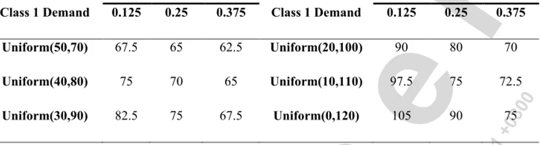
(26) alınmalı. Sayfa 88’de “Proof of Proposition 3” yazısı birleşik yazılmış, ara boşlukları konacak. Makalenin son sayfasında (89.sayfa) Proof of proposition 8’den bittikten sonra aşağıdaki tablo yer alacak.. İktisat İşletme ve Finans 30 (347) Şubat / February 2015 Table 1. Optimal protection levels for Figures 6 and 7. 0.25. 0.375. Class 1 Demand. 0.125. 0.25. 0.375. Uniform(50,70). 67.5. 65. 62.5. Uniform(20,100). 90. 80. 70. Uniform(40,80). 75. 70. 65. Uniform(10,110). 97.5. 75. 72.5. Uniform(30,90). 82.5. 75. 67.5. Uniform(0,120). 105. 90. 5/0 :0 rih Ta 6], 11 .2.. 9.1. 79. ge. 6/2. 120. İnd. ire. n:. [B. ilk. en. :[ 13. IP i], es sit er. tÜ niv. il. 1. 7:2 1. 75. 4:1. 01. 51. se. l. 0.125. +0 30 0. Price ratio. Class 1 Demand. B. İndiren: [Bilkent Üniversitesi], IP: [139.179.2.116], Tarih: 05/06/2015 14:17:21 +0300. Price ratio.

(27)