Paralog-specific gene copy number discovery within segmental duplications

PARALOG-SPECIFIC GENE COPY

NUMBER DISCOVERY WITHIN

SEGMENTAL DUPLICATIONS

a thesis submitted to

the graduate school of engineering and science

of bilkent university

in partial fulfillment of the requirements for

the degree of

master of science

in

computer engineering

By

Emre Do˘

gru

September 2019

PARALOG-SPECIFIC GENE COPY NUMBER DISCOVERY WITHIN SEGMENTAL DUPLICATIONS

By Emre Do˘gru September 2019

We certify that we have read this thesis and that in our opinion it is fully adequate, in scope and in quality, as a thesis for the degree of Master of Science.

Can Alkan(Advisor)

A. Erc¨ument C¸ i¸cek

Tunca Do˘gan

Approved for the Graduate School of Engineering and Science:

Ezhan Kara¸san

ABSTRACT

PARALOG-SPECIFIC GENE COPY NUMBER

DISCOVERY WITHIN SEGMENTAL DUPLICATIONS

Emre Do˘gru

M.S. in Computer Engineering Advisor: Can Alkan

September 2019

With the advancing technology in genome sequencing and analysis, it has become evident that the structural variations are the main source of alteration in human genome. Despite their significance in understanding disease susceptibility, there is no algorithm yet to find all types and sizes of structural variations at once. Structural variation discovery remained problematic since they often overlap with the segmental duplications, nearly identical segments of DNA that appear more than once in the genome. Researchers often excluded these regions that made up ∼5% of the genome because of the complexity it brings to their studies. Only few of them are working in these regions, however, they require a special sequence alignment file where reads are mapped to multiple locations.

Here, we present ParaCoND to discover paralog specific gene copy number within segmental duplications using a sequence alignment file with unique map-ping. We utilize the singly unique nucleotides (SUN) that distinguish paralogs from each other in the sequence alignment of the duplicated regions. Our method is based on read depth and is limited to detect only duplications and deletions. We computed the absolute copy numbers of genes using only read depth of SUN. Furthermore, we also computed the paralog specific absolute copy numbers for genes residing in the same segmental duplication.

Keywords: Structural Variation, Segmental Duplication, Copy Number Variation, Singly Unique Nucleotide.

¨

OZET

SEGMENTAL DUPL˙IKASYONLARDA

PARALOG- ¨

OZG ¨

U KOPYA SAYISI VARYASYONU

KES

¸F˙I

Emre Do˘gru

Bilgisayar M¨uhendisli˘gi, Y¨uksek Lisans Tez Danı¸smanı: Can Alkan

Eyl¨ul 2019

Genom dizileme ve analizinde geli¸sen teknolojiyle birlikte, insan genomundaki de˘gi¸simlerin ana kayna˘ginin yapısal varyasyonlar oldu˘gu belirginle¸sti. C¸ e¸sitli hastalıklara yol a¸cması bakımından ¨onemli olmalarına ra˘gmen, halen b¨ut¨un tip ve uzunluktaki yapısal varyasyonları bulan bir algoritma bulunmamaktadır. Yapısal varyasyon ke¸sfi problemli bir alan olarak kalmı¸stır ¸c¨unk¨u sıklıkla segmental du-plikasyonların, DNA ¨uzerinde birden fazla bulunan y¨uksek oranda benzerlik g¨osteren segmentler, ¨uzerinde bulunmaktadır. Ara¸stırmacılar b¨ut¨un genomun ∼%5’ine kar¸sılık gelen bu b¨olgeleri ara¸stırmalarda karma¸sıklık getirece˘gi i¸cin kap-sam dı¸sında bırakmı¸stır. Sadece birazı bu alanlarda ¸calı¸sma yapmı¸stır, ancak onlar da okumaların birden fazla lokasyonla e¸sle¸stirildi˘gi ¨ozel bir dizi hizalama dosyası kullanmı¸stır.

Bu ¸calı¸smada okumaların tek bir lokasyonla e¸sle¸stirildi˘gi dizi hizalama dosyası kullanarak segmental duplikasyonlarda paralog-¨ozg¨u kopya sayısı varyasyonu ke¸sfi yapan ParaCoND algoritmasını sunuyoruz. Tekrarlı b¨olgelerdeki paralogları bir-birinden ayıran tekli ¨ozel n¨ukleotidleri (T ¨ON) kullanıyoruz. Metodumuz okuma derinli˘gine dayanmaktadır ve sadece duplikasyon ve silme i¸slemlerini tespit et-mekle sınırlıdır. Genlerin mutlak kopya sayılarını sadece T ¨ON okuma derinli˘gini kullanarak hesapladık. Ayrıca, aynı segmental kopyada bulunan genler i¸cin par-aloga ¨ozg¨u mutlak kopya numaralarını da hesapladık.

Anahtar s¨ozc¨ukler : Yapısal Varyasyon, Segmental Duplikasyon, Kopya Sayısı Varyasyonu, Tekli ¨Ozel N¨ukleotid.

Contents

1 Introduction 1

1.1 DNA Sequencing . . . 2

1.1.1 Early Sequencing Methods . . . 2

1.1.2 High-Throughput Sequencing . . . 3

1.2 Genomic Variation . . . 4

1.2.1 Single Nucleotide Polymorphism . . . 4

1.2.2 Structural Variation . . . 5

1.2.3 Chromosomal Changes . . . 6

1.3 Our Contribution . . . 7

2 ParaCoND: Paralog-specific Gene Copy Number Discovery 8 2.1 Structural Variation Discovery with HTS Data . . . 8

2.1.1 Read Pair . . . 9

CONTENTS vii 2.1.3 Split Read . . . 10 2.1.4 Sequence Assembly . . . 11 2.1.5 Hybrid Methods . . . 11 2.2 Dataset . . . 12 2.3 Data Preprocessing . . . 12

2.4 Singly Unique Nucleotides . . . 13

2.4.1 Extracting Singly Unique Nucleotides . . . 13

2.5 Depth of Singly Unique Nucleotides . . . 14

2.5.1 GC Correction . . . 16

2.6 Gene Copy Number . . . 18

2.7 Paralog Gene Copy Number . . . 18

2.7.1 Paralog Specific Copy Number . . . 19

3 Experimental Results 24 3.1 Fluorescent in situ hybridization (FISH) Validation . . . 25

3.2 Reference Genome Simulation with ART . . . 25

3.3 Real Datasets . . . 26

3.4 Results . . . 26

CONTENTS viii

4.1 Future Directions . . . 37

A Data 45

List of Figures

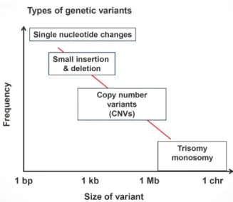
1.1 Size of different genomic variants with respect to their frequency. . 5

2.1 Structural variation discovery with read pair. Paired-end reads that are mapped too distant from each other indicates deletion, too close to each other indicates insertion and ahead of what should be behind indicates inversion (adapted from [1]). . . 9

2.2 Structural variation discovery with read depth.The depth of re-gions that are duplicated will be higher and the depth of rere-gions that are deleted will be lower than expected depth. . . 10

2.3 Workflow figure of ParaCoND. . . 21

2.4 Singly unique nucleotides and paralog specific variants. Singly unique nucleotides are single nucleotide differences among segmen-tal duplications. If there are more than one paralog that contains a nucleotide difference, it will be called a paralog specific variant (adopted from [2]). . . 22

2.5 A sample screenshot from an alignment file. . . 22

LIST OF FIGURES x

2.7 The average depth of 1 kb windows with respect to their GC con-tent for NA12878. . . 23

3.1 Comparison of results with synthetic data generated from refer-ence genome. We used ART, a tool that generates random next-generation sequencing reads from assembled genome. The data was sorted by the results of mrCaNaVaR. . . 29

3.2 Absolute copy numbers of genes overlapping with segmental du-plications. . . 30

3.3 Absolute copy numbers of genes that are 90% or more in the neigh-borhood by both methods. . . 31

3.4 Absolute copy numbers of genes that are 50% or more in the neigh-borhood by both methods. . . 32

3.5 Absolute copy numbers of genes whose copy numbers are less than 10 according to mrCaNaVaR. . . 33

3.6 Absolute copy numbers of genes whose copy numbers are between 10 and 20 according to mrCaNaVaR. . . 34

3.7 Absolute copy numbers of genes whose copy numbers are greater than 20 according to mrCaNaVaR. . . 35

List of Tables

3.1 Comparison of mrCaNaVaR and ParaCoND with validated results obtained from FISH analysis. . . 25

3.2 Comparison of ParaCoND and mrCaNaVaR . . . 27

List of Algorithms

1 An algorithm to find missing SD pairs . . . 12

2 An algorithm to find pairwise SUN locations and letters . . . 15

3 An algorithm to find all SUN locations and letters . . . 16

4 An algorithm to find depth of SUN locations . . . 17

5 An algorithm to find gene copy number . . . 18

Chapter 1

Introduction

It all started with Darwin’s book of The Origins of Species, which he published in 1859. Since then, the field of genomics have been paid a great deal of attention. With the advancing power of computers, the genomic studies had to adapt itself into this new circumstances. The Human Genome Project was started in 1990 with the goal of determining all the bases in human genome. This was not only exciting but also difficult goal to reach since it could take years or decades to sequence the whole genome with the existing technology. As expected, after 13 years of hard work, the results were published in 2003, and it cost $2.7 billion [3].

The main sequencing method that was used in Human Genome Project was Sanger’s chain termination method, or commonly referred to as Sanger sequenc-ing. Sanger sequencing, named after the inventor Frederick Sanger, was good in terms of accuracy, however, it was time-consuming and expensive. In the early 2000s, methods that were better at time and money were finally emerging. Next-generation or high-throughput methods have revolutionized the sequencing business by providing millions of “reads”, short sequences, in a massively parallel fashion at a lower cost. As high-throughput sequencing (HTS) methods have be-come widespread, an effort to make available as many human genomes as possible was set out. For instance, started in 2008, 1000 Genome Project aimed to se-quence approximately 2500 individual coming from different ethnic backgrounds

[4]. Several countries, among them are Turkey, have started their own genome projects. In addition to human genome, genomes belonging to other species have also been sequenced [5].

1.1

DNA Sequencing

Before 1950s, the term “gene” was referred to as the smallest unit of genetic information [6]. Scientists at that time were identifying the DNA as the carrier of genetic information, however, they knew very little about how a trait passes down to younger generations. In 1953, there was a breakthrough in the field of genomics with the discovery of double helix structure of DNA by James Watson and Francis Crick. Watson and Crick had answered the biggest question till then in genomics that could lead to solving the mystery about genetic heredity. In a series of articles published in several journals, Watson et al., apart from exposing the structure of DNA, have put their findings together with those of other researchers and come up with a mechanism for DNA replication along with three pieces of evidence supporting the complementary model which suggests that adenine has thymine and cytosine has guanine on the opposite strand of DNA, or vice versa [7].

1.1.1

Early Sequencing Methods

The complementary model opens the door of DNA sequencing since it allows the DNA to be reconstructed from one strand. There were some initial thoughts and methods on how to sequence the DNA, however, none of them were practical in terms of speed to sequence the whole genome. Frederick Sanger and Alan Coulson were the first who have developed the “plus and minus” method, which was soon replaced by chain-termination method, for rapidly determining the order of smallest genetic units in DNA[8]. In an article published in 1970, Sanger et al. have set the gold standard in sequencing. They used DNA polymerase, an enzyme that is essential for DNA replication, to generate copy DNA sequences from the

template DNA strand, all of which should start in the same exact position and end in normally one base larger (and heavier) than the previous. Sanger was able to stop the polymerase by removing an oxygen from the nucleotide at which he wants to stop. Sanger made these DNA sequences move at a speed such that the fewer nucleotides they have, the faster they are. Nucleotides will emit a light in different wavelengths, hence, from a fixed point of view, a light sensor will be able to detect the sequence of nucleotides.

1.1.1.1 Human Genome Project

As the technology in DNA sequencing advances, it has become a must to sequence the whole human genome. After two years of preparation and planning, Human Genome Project (HGP), an international research project, was officially started in 1990 with two simple goals. Along with the purpose of determining all the bases in human DNA, they had also wanted to find out the mapping of the genes in human genome. In 1998, a private company called Celera Genomics have announced that they entered the race to sequence human genome. The competitor have made HGP researchers to speed up their efforts. After eleven years from the start, 90% of human DNA sequence was published in February 2001. The project was officially over in 2003 with 99% of the genome have been published with an error rate of 0.01%.

The results were gathered from the genome of 7-8 individuals to provide re-searchers with a good approximation of human DNA, which is called the “refer-ence genome”. The refer“refer-ence genome is regularly updated by Genome Refer“refer-ence Consortium and useful in genome assembly.

1.1.2

High-Throughput Sequencing

For about 40 years since the invention, Sanger sequencing have been the dominant sequencing method with slight modifications. It was the main sequencing method used in HGP. The experience acquired from HGP have made clear that, despite

its accuracy and provision of long reads, Sanger sequencing was costly and slow.

High-throughput sequencing, on the other hand, have addressed these issues by processing millions of DNA fragments in parallel. Thanks to HTS, cost and time of sequencing a human genome decreased enormously. In 2001, the cost of sequencing a genome was $100 million and it took 13 years. With today’s technology, a human genome could be sequenced for around $1300 [3] in a couple of days [9].

Despite its success in terms of time and money over Sanger sequencing, higher sequencing error rates, shorter read lengths and bias against GC-rich regions [10] are among HTS platforms’ drawbacks researchers had to deal with.

1.2

Genomic Variation

With the hundreds of thousands human genome have become accessible, re-searchers have become interested more in the question of what makes one in-dividual different than the other. Early research results have suggested that 99.9% of human genome is identical. Among 3 billion bases making up the hu-man genome, it was only 3 million bases where all the differences between huhu-mans were attributed to. Figure 1.1 shows the inverse correlation between the size of genetic variants and their frequencies in the genome. As the genomic variant is getting larger, it can rarely be seen. It has become evident that genetic variants are the reason for many disease including color blindness [11], psoriasis [12], HIV susceptibility [13], Crohn’s disease [14] and many more [15].

1.2.1

Single Nucleotide Polymorphism

Single nucleotide polymorphism, SNP for short, is a substitution at a specific position in the DNA sequence. A substitution can be called a SNP if and only if it is the case for more than 1% of the population. The implications of a SNP

Figure 1.1: Size of different genomic variants with respect to their frequency.

can be significant especially if it exists in a coding region of the DNA. A SNP can change the translation of a codon into an amino acid, what is called a non-synonymous mutation, causing a distortion in the structure of the protein.

1.2.2

Structural Variation

Structural variations (SV) are rearrangements in human genome affecting more than 50 bp that could reach up to several megabases. Structural variations can be categorized according to whether they alter the amount of DNA (copy number variations) or not (balanced rearrangements).

1.2.2.1 Copy Number Variation (CNV)

Copy number variation, also known as unbalanced rearrangement, is a structural variation that changes the amount of DNA. CNVs are also seperated into two:

• Insertions and Deletions: As the name suggests, these are insertions or deletions affecting more than 50 bp.

• Segmental Duplications: They are segments in the DNA that are more than 1000 basepair and 90% or more identical. It can be intra-chromosomal as well as inter-chromosomal. Although segmental duplications account for ∼5% of the genome, they are significant because (1) they often exist in gene-rich chromosomes [16] and (2) they are the most active regions in human genome triggering instabilities and new variations in the chromosome [17, 2].

1.2.2.2 Balanced Rearrangements

Balanced rearrangements are structural variations that do not change the amount of DNA. Balanced rearrangements can be categorized into two;

• Inversions: They are rearrangements where a segment of the DNA is simply inverted.

• Translocations: They are rearrangements where two segments of the DNA exchange their locations.

1.2.3

Chromosomal Changes

Chromosomal changes are variations in the number of chromosome-pairs. They are such major variations that they can be detected by a microscope. It can be categorized into three:

• Monosomy: It is a chromosomal change where there is only one copy of a chromosome.

• Trisomy: It is a chromosomal change where there is an extra copy of a chromosome.

• Uniparental Disomy: It is a chromosomal change where both pairs of chro-mosome come from the same parent.

1.3

Our Contribution

In this thesis, we present ParaCoND to discover paralog specific copy numbers for genes residing in segmental duplications. This remains an open problem until mrCaNaVaR [18] came out, due to the difficult nature of duplicated regions in genome. However, mrCaNaVaR was not good at differentiating the paralogs. Instead it computes aggregate copy number and assigns it to different copies of genes. Accurate prediction of paralog gene copy number could pave the way of finding the main causes of genetic diseases. For example; opsin is a gene family responsible for color vision. It has three copies that regulate color vision according to wavelengths of different colors. Therefore a variation on a paralog could have an effect on viewing colors of specific wavelengths.

The main improvement of ParaCoND over mrCaNaVaR is that our method utilizes single nucleotide differences among paralogs which helps us to differentiate paralogs from each other. In addition to that, mrCaNaVaR requires a multiple read mapping sequence alignment file, which is not as widespread as unique read mapping. Our method compute the absolute copy numbers of genes residing in segmental duplications using a unique mapping sequence alignment file.

The organization of the thesis is as follows: We briefly introduced the problem in Chapter 1. We further explain the problem and present our method in Chapter 2. We show the experimental results in Chapter 3. We conclude the thesis with final remarks in Chapter 4.

Chapter 2

ParaCoND: Paralog-specific

Gene Copy Number Discovery

In this chapter, each step that we followed in our method will be explained in detail.

2.1

Structural Variation Discovery with HTS

Data

Structural variations are believed to be highly associated with diseases [19, 14, 15, 13]. Therefore their discovery will be of critical importance in reducing the genetic disease susceptibility. Despite their significance in understanding disease susceptibility, there is no algorithm yet to find all types and sizes of structural variations at once. Before high-throughput sequencing technologies, microarrays were mainly used in structural variation discovery especially for copy number variation [20]. As reviewed by Alkan et al., microarrays are not good at discov-ering balanced rearrangements and also are not able to locate the copy number variations [20].

Although some are originally designed for old sequencing technologies, high-throughput sequencing platforms have brought novel methods for structural vari-ation discovery.

2.1.1

Read Pair

Paired-end sequencing is a sequencing method where reads are generated from both sides of a DNA fragment whose distance is known. The distance informa-tion will be used later by the aligner while aligning the paired-end reads to the reference genome. Read pair method utilizes the distance information between paired-end reads [1]. As shown in the Figure 2.1, paired-end reads that align too distant from each other indicates a deletion, those align too close to each other indicates an insertion.

Figure 2.1: Structural variation discovery with read pair. Paired-end reads that are mapped too distant from each other indicates deletion, too close to each other indicates insertion and ahead of what should be behind indicates inversion (adapted from [1]).

Structural variation discovery tools based on read-pair can be categorized as follows:

• Unique Mapping: PEMer [21], BreakDancer [22], GenomeSTRIP [23],

• Multiple Mapping: VariationHunter [24], CommonLAW [25], MoDIL [26], MoGUL [27], HYDRA [28]

2.1.2

Read Depth

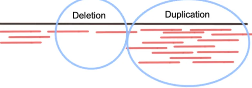
Read depth is a simple method to detect duplications and deletions. Based on the assumption that regions are randomly sequenced, for reads that are mapped to the reference genome, the depth of duplicated regions will be higher and the depth of deleted regions will be lower than average [16] as shown in Figure 2.2. Multiple read-mapping is an important aspect of read depth to work effectively. Otherwise the difference of depth between duplicated regions and deleted regions will be insignificant. However known sequencing bias against rich and GC-poor regions [10] should be handled carefully.

Figure 2.2: Structural variation discovery with read depth.The depth of regions that are duplicated will be higher and the depth of regions that are deleted will be lower than expected depth.

Structural variation discovery tools based on read depth can be categorized as follows:

• Unique Mapping: CNVnator [29], Event-Wise Testing [30]

• Multiple Mapping: Whole Genome Shotgun Sequence [16], mrCaNaVaR [18]

2.1.3

Split Read

Originally designed for longer reads (Sanger sequence etc.), split read based meth-ods were capable of structural variation discovery at one base pair resolution by

trying to map the reads by splitting. Similar to read pair, the location of split reads will tell the class of structural variation. For instance, the distance between split reads shows an insertion or first split coming after second split indicates an inversion.

Structural variation discovery methods based on split read can be categorized as follows:

• Unique Mapping: Pindel [31], SRiC [32]

• Multiple Mapping: Splitread [33]

2.1.4

Sequence Assembly

Although it is in its early stages, sequence assembly methods are, in theory, powerful and requires less computational power. Assuming the whole genome is assembled without using the reference genome (de novo assembly), we can easily detect structural variation by comparing the individual’s genome with the reference genome. NovelSeq [34], PopIns [35] can be examples of this type.

2.1.5

Hybrid Methods

There are also some methods using two or more of these techniques in order to increase their accuracy. Examples of these type of methods can be DELLY [36] in which read pair and split read were used, LUMPY [37] in which read pair, read depth and split read were used, TARDIS [38] in which read pair, read depth and split read were used.

2.2

Dataset

We have the data showing the genome-wide segmental duplications (SD). The data is coming from Segmental Duplication Database of UW Genome Sciences Human Paralogy Laboratory [39, 16]. The data consist of 51,599 SD pairs with their exact locations. Furthermore, we have global alignments of SD pairs in files generated using a sequence alignment tool called ClustalW [40].

2.3

Data Preprocessing

Since entries in our data show the duplications in pairs, we had to turn these pairs into a multiple sequence alignment in order to locate singly unique nucleotide positions. However, our data lack some pairs. For example, we have SD pairs of A-B and B-C, therefore A-C should also be in our data whereas there is not in some cases. Using the Algorithm 1, we have identified 21,023 new SD pairs using existing pairs and have them aligned.

Algorithm 1 An algorithm to find missing SD pairs

1: _{procedure Find Missing Pairs}

2: M ← map of Segmental Duplications as read from data

3: for each key-value pair in M do

4: Let temp set be an empty set

5: for values in M[key] do

6: temp set ← temp set ∪ M[value]

7: clear M[value]

8: while true do

9: flag ← true

10: for each key-value pair in M do

11: Find intersection of temp set and value

12: if intersection is not empty then

13: temp set ← temp set ∪ M[value] 14: flag ← false

15: if flag is true then

2.4

Singly Unique Nucleotides

Structural variation discovery has always been problematic since they tend to overlap with segmental duplications [2]. Researchers that were unable to dis-criminate slight differences in these regions which prevents copy number variation from being accurately predicted have excluded these highly active regions from their studies. They have instead focused on unique regions of the genome.

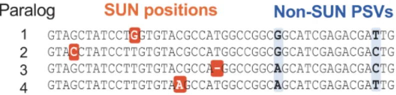
In nearly identical regions, nucleotide difference information can be useful in discriminating segmental duplications from each other. Singly unique nucleotide (SUN) is a nucleotide difference between segmental duplications as shown red in Figure 2.4. A nucleotide difference is called a SUN if and only if they reside in only one paralog. Otherwise, as shown blue in the Figure 2.4, they are called paralogous sequence variant (PSV).

2.4.1

Extracting Singly Unique Nucleotides

In order for paralogous sequences to be accurately identified, we need a database of positions and letters of all SUNs that reside in a segmental duplication. Instead of aligning paralogs using a multiple sequence alignment tool, which requires quite some time and computational power, it could be done using pairwise alignments of paralogs which we have in our hand (Figure 2.5). Let A, B and C are three paralogs and Sab denotes the singly unique nucleotides of A relative to B. The

singly unique nucleotides of A will be Sab∩ Sac. The same equation is valid for

other paralogs respectively. Therefore, we could figure out all SUN positions as (Sab∩ Sac) ∪ (Sba∩ Sbc) ∪ (Sca∩ Scb).

Algorithm 2 uses an alignment file to find the pairwise SUN positions and letters. As shown in Figure 2.5, an alignment file contains the DNA sequences of two segments and an alignment results between them. The symbols ∗, | and space denote a match, a mismatch and an indel respectively. It is important to state that, if there is a deletion in one sequence, every nucleotide position opposite of

the deletion will be counted as a SUN. On the other hand, the deletion will be counted as one SUN. Another thing to pay attention is the strand of the sequences. Segmental duplications can be found in opposite strand of the DNA. In that case, the nucleotide in the alignment file will be replaced by its complement before getting saved to SUN database.

In algorithm 3, we use algorithm 2 to create a SUN database of segmental duplications by intersecting relative SUN sets. First we find SUNs of A relative to B and SUNs of B relative to A. And then, if A or B come out for the first time, we save the relative SUNs directly to the sun map since there is no set of SUNs yet to intersect. On the other hand, if A or B is found in sun map, we intersect the old set of SUNs with the relative SUNs. We store the database in a map where its keys are segmental duplications and its values are SUN locations and letters.

As a result, we have found 15,352,106 unique SUN locations together with their bases on a positive strand of the DNA.

2.5

Depth of Singly Unique Nucleotides

The depth or coverage, a term that entered the literature thanks to the next generation sequencing, is defined as the number of ‘reads’ that include a particular nucleotide. In next generation sequencing, the DNA is separated into little and overlapping portions, called ‘reads’, to be assembled later. When the reads are aligned with respect to their mapping locations, nucleotides are sequenced in varying numbers as shown in Figure 2.6. Therefore the number the nucleotide gets sequenced is called the depth of that position.

As explained in Section 2.4, we have created a SUN database showing all the SUN locations. In Algorithm 4, we basically compute the depth of SUN locations if base in ‘read’ matches with the base of SUN. In order to use this function, we need a BAM file as a parameter. BAM [41] is a file type for storing sequence

Algorithm 2 An algorithm to find pairwise SUN locations and letters

1: _{procedure Get Relative SUN(alignment file path, strand)} 2: Open alignment file

3: if file is open then

4: Let Sab and Sba empty sets

5: while getline(file) 6= EOF do

6: seq1 ← getline(file)

7: aligment ← getline(file)

8: seq2 ← getline(file)

9: for i ← 0 to size of alignment do

10: if strand is − 1 then

11: seq2[i] ← GET OPPOSITE PAIR(seq2[i]) /* It

12: returns the complement of the input nucleotide, for example

13: if input is A, T is returned etc.*/

14: if alignment[i] is ‘*’ then 15: Sab ← Sab∪ seq1[i] 16: Sba ← Sba∪ seq2[i] 17: if alignment[i] is ‘ ’ then 18: if seq1[i] is ‘-’ then 19: Sba ← Sba∪ seq2[i] 20: if seq2[i] is ‘-’ then 21: Sab ← Sab∪ seq1[i]

Algorithm 3 An algorithm to find all SUN locations and letters

1: _{procedure Get All SUN(duplication file path)} 2: Open duplication file

3: if file is open then

4: Let sun map an empty map showing segmental duplication and

5: its SUN locations as key-value pair

6: for each entry in duplication file do

7: Let A, B segmental duplications as parsed from duplication file

8: alignment file path ← parsed from duplication file

9: strand ← parsed from duplication file

10: Sab, Sba ← GET RELATIVE SUN(alignment file path, strand)

11: if A exists in sun map then

12: sun map[A] ← sun map[A] ∩ Sab

13: else

14: sun map[A] ← Sab

15: if B exists in sun map then

16: sun map[B] ← sun map[B] ∩ Sba

17: else

18: sun map[B] ← Sba

alignment data in binary format. For each alignment it contains read name, read sequence, read quality, alignment information, and custom tags. We used HTSLib [42], a C library for reading/writing high-throughput sequencing data, to efficiently read a BAM file.

2.5.1

GC Correction

The next generation sequencing platforms are known to be biased against regions that are rich or poor in terms of GC content [10]. This has been a known issue of HTS platforms that lead to uneven or even no coverage of reads across the genome. Unless it was handled carefully, structural variation discovery meth-ods that rely on coverage data would not be applicable. Fortunately, there are statistical methods out there to fix the uneven distribution of reads. We used multiplicative version of locally weighted scatter plot smooth [43], LOWESS or LOESS in short, to smooth our GC content vs read depth curve. The method

Algorithm 4 An algorithm to find depth of SUN locations

1: _{procedure Find Depth(bam file, sun set)} 2: Open bam file

3: if file is open then

4: for every read in bam file do

5: chr ← parsed from bam file

6: pos ← parsed from bam file

7: len ← parsed from bam file

8: seq[len] ← CONVERT ID TO NUCLEOTIDE // In a bam file,

9: each base is encoded in 4 bits: 0001: A, 0010: C, 0100: G,

10: 1000: T, 1111: N. This procedure converts the binary-coded

11: nucleotide to its letter representation.

12: for each SUN falling into the ‘reads’ range do

13: if seq[SUN index] is equal to SUN nucleotide then

14: Increment depth of SUN by 1

15: else

16: Remove from sun set

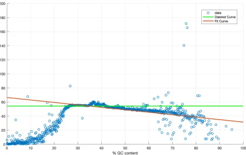
starts with computing the average read depth of non-overlapping sequence win-dows of size 1 kilobase. Then the sequence winwin-dows are binned according to their GC percentage. There is 0.1% difference between two consecutive bins. And again we compute the average read depth for each bin.

The Figure 2.7 shows how the average read depth is impacted by GC content. The average read depth are getting lower with increasing GC content. We need to adjust the red line so that it comes closer to the green line. In multiplicative version of LOESS method, we define a correction factor, kgc, which is equal to

kgc =

µtotal

µgc

where µtotal is the average read depth of all sequence windows (i.e. green line)

and µgc is the fit curve smoothed by LOESS (i.e. red line). Having computed kgc

for all GC percentages and known the old value for read depth d, new value for read depth, d0, is calculated as;

d0 = d ∗ kgc

2.6

Gene Copy Number

Copy number variation is a structural variation that changes the amount of DNA. The simple yet powerful method for finding absolute copy number of a region is read depth. However, without multiple read mapping, applying read depth will give poor results. What we compute here is a copy number that will be useful later while computing the paralog specific copy number.

Algorithm 5 An algorithm to find gene copy number

1: _{procedure Find Gene Copy Number(gene file path, sun set)} 2: Let Genes be a vector of genes as read from gene file path

3: for each gene in Genes do

4: Let temp be empty vector

5: for each SUN in sun set do

6: if SUN is in gene then

7: Add read depth of SUN to temp

8: if temp is not empty then

9: Compute mean and median of temp

In algorithm 5, we try to find average gene copy numbers using only the depth information of SUNs residing in that gene. The procedure takes two parameters. One is the gene file path, the file that contains gene location information of refer-ence genome version GRCh37 (hg19). The other is sun set produced by previous algorithms with read depth information.

As a result of the algorithm 5, we found 4279 genes that has at least one SUN on them and therefore an average copy number can be calculated for them. These genes are residing in a segmental duplication which makes them paralog genes.

2.7

Paralog Gene Copy Number

Paralog genes are genes that are related as a result of duplication [44]. Unlike orthologs, paralog genes do not have to have the same functionality, however, it can be related since they are coming from a common ancestor. Paralog genes are

important factors of genomic evolution [45].

Computing paralog specific copy number is important since they can be asso-ciated with disease or phenotypes. For instance opsin is a gene family that is re-sponsible for color vision with 3 genes, namely OPN1LW (long wave), OPN1MW (medium wave), and OPN1SW (short wave). Mutations in this gene family can cause color blindness. More specifically, genomic variations in OPN1LW can cause reduction in color vision for colors whose wavelength is long in the vis-ible spectrum such as red or orange. Likewise, a variation in OPN1MW can cause yellow-green blindness, and a variation in OPN1SW can cause blue-violet blindness.

2.7.1

Paralog Specific Copy Number

Paralog genes show more variation in copy number than those that are non-paralog since they exist in duplicated regions. We determine non-paralog genes ac-cording to whether they reside in a segmental duplications or not. If a gene is in a segmental duplication, it means it has a paralog on other copies.

Algorithm 6 An algorithm to find paralog specific copy number

1: _{procedure Find Paralog Specific Copy Number(gene file path,}

seg-mental duplication file path)

2: SegmentalDuplications ← parsed from segmental duplication file path

3: Genes ← parsed from gene file path

4: for each segDup in SegmentalDuplications do

5: totalCNV ← 0

6: for each gene in Genes do

7: if gene is on segDup then

8: totalCN V ← totalCN V + gene.getCN V ()

In algorithm 6, we try to compute paralog specific copy number of paralog genes. Since we use a sequence alignment file in which the reads were mapped to a single location by the aligner, the average copy number of genes are expected to be lower. Therefore we sum the average copy numbers of genes that are on the same segmental duplication (i.e. paralog). The result will be the absolute copy

Figure 2.3: W orkflo w figure of P araCoND.

Figure 2.4: Singly unique nucleotides and paralog specific variants. Singly unique nucleotides are single nucleotide differences among segmental duplications. If there are more than one paralog that contains a nucleotide difference, it will be called a paralog specific variant (adopted from [2]).

Figure 2.5: A sample screenshot from an alignment file.

Figure 2.7: The average depth of 1 kb windows with respect to their GC content for NA12878.

Chapter 3

Experimental Results

In this chapter, we present the results that we acquired while testing our method. We tested our method in three different ways. First, we used experimentally val-idated copy numbers from [18]. They are valval-idated by the fluorescent in situ hybridization (FISH) method, which is commonly used to test whether a spe-cific chromosome region is present or not. Second, we used the tool ART [46] to generate synthetic next-generation sequencing reads from the reference genome. Since reference genome is known to be free of copy number variation, we ex-pect our method to compute copy numbers around 2. And lastly we tested our method with real datasets collected from 1000 Genome Project[47] and Turkish Genome Project [48]. Since there is no complete validated results for paralog genes, we compare our results with the results of mrCaNaVaR [18], a tool to dis-cover structural variations in duplicated regions. mrCaNaVaR, like our method, was based on read depth and it was designed to determine absolute copy numbers in duplicated regions [49].

3.1

Fluorescent in situ hybridization (FISH)

Validation

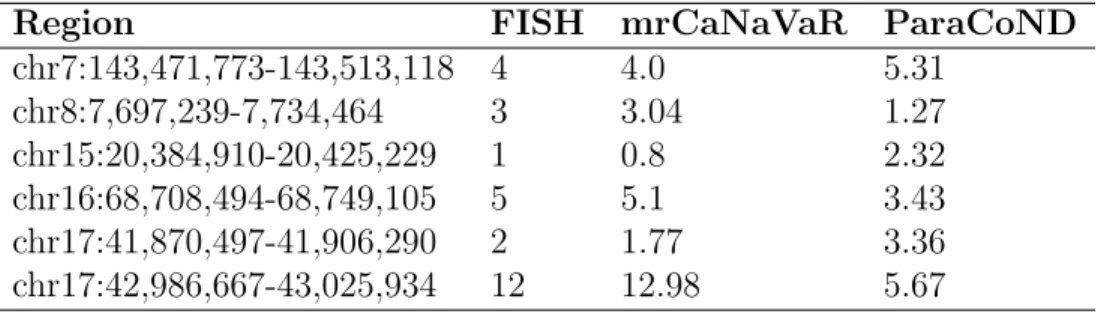
Fluorescent in situ hybridization (FISH) is a technique developed in 1982 by Langer-Safer et. al. to detect the presence or absence of specific DNA sequence [50]. Alkan et. al. performed FISH analysis on selected regions of genome NA18507 from 1000 Genome Project [18, 47]. Table 3.1 shows the performance of ParaCoND over mrCaNaVaR with FISH validated data.

Table 3.1: Comparison of mrCaNaVaR and ParaCoND with validated results obtained from FISH analysis.

Region FISH mrCaNaVaR ParaCoND chr7:143,471,773-143,513,118 4 4.0 5.31 chr8:7,697,239-7,734,464 3 3.04 1.27 chr15:20,384,910-20,425,229 1 0.8 2.32 chr16:68,708,494-68,749,105 5 5.1 3.43 chr17:41,870,497-41,906,290 2 1.77 3.36 chr17:42,986,667-43,025,934 12 12.98 5.67 FISH analysis results was taken from [18].

3.2

Reference Genome Simulation with ART

Reference genome is a good approximation of human genome without any vari-ation. We used ART [46], a tool that generates synthetic next-generation reads from assembled genome, to generate random reads from reference genome. Then we realigned them to reference genome using BWA-MEM [51] in order to create a variation-free sequence alignment file.

Figure 3.1 shows the results gathered from both methods using the synthetic data generated from reference genome. Since mrCaNaVaR computes aggregate copy number for paralogs, it can be expected mrCaNaVaR to compute higher than 2. On the other hand, ParaCoND outperforms mrCaNaVaR in this dataset by computing gene copy numbers around 2.

3.3

Real Datasets

We tested ParaCoND with two human genomes: NA12878 from 1000 Genome Project and 42S291210 from Turkish Genome project. In general, 30X sequenc-ing coverage is adequate for clinical-level research [52]. Therefore we picked one genome (NA12878) [47] as an example of a human genome sequence with a high coverage (43 times) and another genome (42S291210) [48] as an example of rela-tively low coverage genome (20 times).

3.4

Results

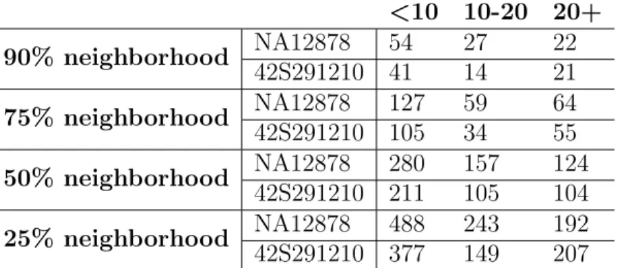
In this section, the results of mrCaNaVaR and ParaCoND are compared via several plots. The results include absolute copy numbers of paralog genes (i.e. genes overlapping with segmental duplications). It is not expected the results to match perfectly, however, they should show some level of consistency. We measure the consistency as neighborhood percentages. The neighborhood percentage is the ratio of absolute copy numbers. For example, we say 90% or more consistent if the following inequality holds;

90 100 ≤ CN VP araCoN D CN VmrCaN aV aR ≤ 100 90 .

Table 3.2 shows the statistics on the level of consistency between ParaCoND and mrCaNaVaR. For NA12878, among 1205 genes for which an absolute copy number is computed by both method, 98 genes show 90% or more in their neigh-borhood and for 42S291210, among 1052 genes, 48 genes show 90% or more in their neighborhood. The reason behind the small difference between two genomes is most likely caused from their sequencing coverage. NA12878 is sequenced 2.15 times more than 42S291210. High sequencing coverage means high quality reads and low sequencing error.

Table 3.2: Comparison of ParaCoND and mrCaNaVaR Neighborhood Percentage NA12878 42S291210

90% or more 103 76

75% or more 250 194

50% or more 561 420

25% or more 923 733

Total 1205 1052

Table entries show the number of genes that are in their neighborhood according to copy number computation by both methods.

numbers. As the absolute copy numbers grows, their neighborhood percentages decreases. This is mainly because the sensitivity of the methods are getting lower when absolute copy number is high.

Table 3.3: Comparison of methods according to copy number values <10 10-20 20+ 90% neighborhood NA12878 54 27 22 42S291210 41 14 21 75% neighborhood NA12878 127 59 64 42S291210 105 34 55 50% neighborhood NA12878 280 157 124 42S291210 211 105 104 25% neighborhood NA12878 488 243 192 42S291210 377 149 207

The entries in the table indicates the number of genes. First column indicates the genes having absolute copy numbers less than 10, second column indicates the genes having absolute copy numbers between 10 and 20 and the third column indicates the genes having absolute copy numbers more than 20 according to mrCaNaVaR.

We compare the results of two methods via several plots. The first three plots show the results with respect to their neighborhood percentages. We also plot the results according to their absolute copy numbers computed by mrCaNaVaR.

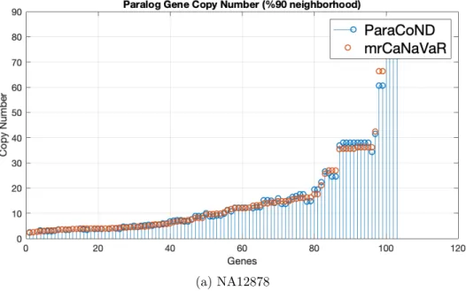
The computed absolute copy numbers for paralog genes by both method can be seen in Figure 3.2. In Figure 3.3, we filter in the genes that are 90% or more in the neighborhood. As can be seen in the figure, most of them have an absolute

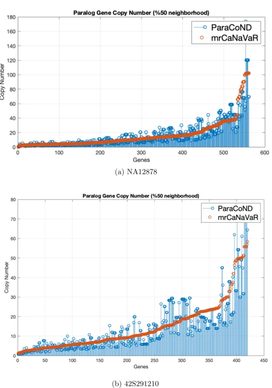
copy number less than 10. Lastly the Figure 3.4 shows the absolute copy numbers computed by both methods in which they are 50% or more in their neighborhood.

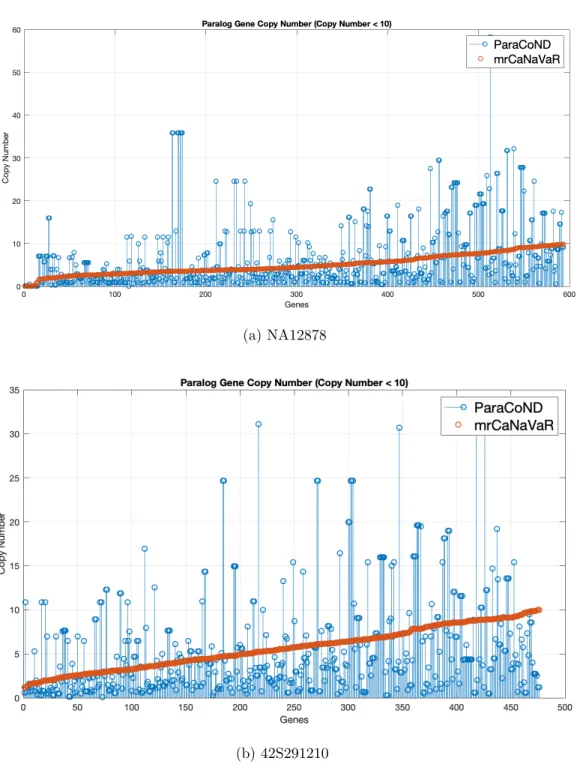
The comparison of computed absolute copy numbers for genes whose copy number is less than 10 can be seen in Figure 3.5. In Figure 3.6, we compare the absolute copy numbers of genes whose copy numbers vary between 10 and 20. We also compare the absolute copy numbers of genes whose copy number greater than 20 in the Figure 3.7.

Figure 3.1: Comparison of results with syn thetic data generated fro m reference genome. W e used AR T, a to ol that generates random next-generation sequencing re ads from assem bled genome. The da ta w as sorted b y the results of mrCaNaV aR.

(a) NA12878 (b) 42S291210 Figure 3.2: Absolute cop y n um b ers of genes o v erlapping with segm en tal dup lications.

(a) NA12878

(b) 42S291210

Figure 3.3: Absolute copy numbers of genes that are 90% or more in the neigh-borhood by both methods.

(a) NA12878

(b) 42S291210

Figure 3.4: Absolute copy numbers of genes that are 50% or more in the neigh-borhood by both methods.

(a) NA12878

(b) 42S291210

Figure 3.5: Absolute copy numbers of genes whose copy numbers are less than 10 according to mrCaNaVaR.

(a) NA12878

(b) 42S291210

Figure 3.6: Absolute copy numbers of genes whose copy numbers are between 10 and 20 according to mrCaNaVaR.

(a) NA12878

(b) 42S291210

Figure 3.7: Absolute copy numbers of genes whose copy numbers are greater than 20 according to mrCaNaVaR.

Chapter 4

Conclusion and Discussion

In this thesis, we present ParaCoND to discover paralog specific gene copy number within segmental duplications. Duplication-rich regions are mostly abandoned from structural variation discovery because of its complex nature. mrCaNaVaR was the first tool to address these problems, however its performance in differ-entiating paralogs from each other is poor and it uses a sequence alignment file where reads are mapped to multiple locations.

In our method, we utilized the singly unique nucleotides in order to differentiate the paralogs from each other. Our method was based on read depth and suffered from GC bias. We solved the problem using multiplicative version of LOESS method. We computed the average copy numbers of genes using read depth of singly unique nucleotides on that gene. And finally we sum the average copy numbers of genes residing in the same segmental duplication to find paralog specific copy number of genes.

Since read depth is limited to detecting duplications and deletions [20], we had to exclude other types of structural variations from our study. Furthermore, the absence of validated results makes us to compare our results with another. Therefore, it was difficult for us to determine ParaCoND’s performance.

4.1

Future Directions

The main obstacle in genomic studies is that the input files are too large to process. In order to reduce storage and computational cost in large scale genome projects, the input files are kept in binary or compressed format (BAM/CRAM). Since multiple read mapping is the key element of mrCaNaVaR, a remapping process should be done with these files which would make duplication analysis costly. Therefore, it is highly likely that methods like ParaCoND that can work with readily available BAM/CRAM files will be regarded as enabling technique for duplication analysis due to its reduced computational cost.

In this thesis, we applied ParaCoND to human genomes. It can be extended to genomes from different organisms. Furthermore, it can also be extended to dif-ferent structural variation types. The latter requires a rather big change since we need to change our main signature (read depth) for structural variation discovery.

The method can be improved in many ways, however, there is an urgent need of a validated data set.

Bibliography

[1] E. Tuzun, A. J. Sharp, J. A. Bailey, R. Kaul, V. A. Morrison, L. M. Pertz, E. Haugen, H. Hayden, D. Albertson, D. Pinkel, et al., “Fine-scale structural variation of the human genome,” Nature genetics, vol. 37, no. 7, p. 727, 2005.

[2] P. H. Sudmant, J. O. Kitzman, F. Antonacci, C. Alkan, M. Malig, A. Tsalenko, N. Sampas, L. Bruhn, J. Shendure, E. E. Eichler, et al., “Diver-sity of human copy number variation and multicopy genes,” Science, vol. 330, no. 6004, pp. 641–646, 2010.

[3] National Human Genome Research Institute, “The cost of sequencing a hu-man genome.” https://www.genome.gov/about-genomics/fact-sheets/ Sequencing-Human-Genome-cost. Accessed: 2019-06-15.

[4] 1000 Genomes Project Consortium and others, “A global reference for human genetic variation,” Nature, vol. 526, no. 7571, p. 68, 2015.

[5] K.-P. Koepfli, B. Paten, G. K. C. of Scientists, and S. J. O’Brien, “The genome 10k project: a way forward,” Annu. Rev. Anim. Biosci., vol. 3, no. 1, pp. 57–111, 2015.

[6] National Institutes of Health, “The francis crick papers: The discovery of the double helix, 1951-1953.” https://profiles.nlm.nih.gov/SC/Views/ Exhibit/narrative/doublehelix.html. Accessed: 2019-06-13.

[7] J. D. Watson and F. H. Crick, “The structure of dna,” in Cold Spring Harbor symposia on quantitative biology, vol. 18, pp. 123–131, Cold Spring Harbor Laboratory Press, 1953.

[8] F. Sanger and A. R. Coulson, “A rapid method for determining sequences in dna by primed synthesis with dna polymerase,” Journal of molecular biology, vol. 94, no. 3, pp. 441–448, 1975.

[9] Illumina, “Run time estimates for each sequenc-ing step on the illumina sequencing platforms.” http: //emea.support.illumina.com/bulletins/2017/02/

run-time-estimates-for-each-sequencing-step-on-illumina-sequenci. html. Accessed: 2019-06-15.

[10] D. R. Smith, A. R. Quinlan, H. E. Peckham, K. Makowsky, W. Tao, B. Woolf, L. Shen, W. F. Donahue, N. Tusneem, M. P. Stromberg, et al., “Rapid whole-genome mutational profiling using next-generation sequencing technologies,” Genome research, vol. 18, no. 10, pp. 1638–1642, 2008.

[11] Genetics Home Reference, “Color vision deficiency.” https://ghr.nlm.nih. gov/condition/color-vision-deficiency. Accessed: 2019-06-17.

[12] E. J. Hollox, U. Huffmeier, P. L. Zeeuwen, R. Palla, J. Lascorz, D. Rodijk-Olthuis, P. C. Van De Kerkhof, H. Traupe, G. De Jongh, M. Den Heijer, et al., “Psoriasis is associated with increased β-defensin genomic copy num-ber,” Nature genetics, vol. 40, no. 1, p. 23, 2008.

[13] E. Gonzalez, H. Kulkarni, H. Bolivar, A. Mangano, R. Sanchez, G. Catano, R. J. Nibbs, B. I. Freedman, M. P. Quinones, M. J. Bamshad, et al., “The influence of ccl3l1 gene-containing segmental duplications on hiv-1/aids sus-ceptibility,” Science, vol. 307, no. 5714, pp. 1434–1440, 2005.

[14] K. Fellermann, D. E. Stange, E. Schaeffeler, H. Schmalzl, J. Wehkamp, C. L. Bevins, W. Reinisch, A. Teml, M. Schwab, P. Lichter, et al., “A chromosome 8 gene-cluster polymorphism with low human beta-defensin 2 gene copy num-ber predisposes to crohn disease of the colon,” The American Journal of Human Genetics, vol. 79, no. 3, pp. 439–448, 2006.

[15] T. J. Aitman, R. Dong, T. J. Vyse, P. J. Norsworthy, M. D. Johnson, J. Smith, J. Mangion, C. Roberton-Lowe, A. J. Marshall, E. Petretto, et al.,

“Copy number polymorphism in fcgr3 predisposes to glomerulonephritis in rats and humans,” Nature, vol. 439, no. 7078, p. 851, 2006.

[16] J. A. Bailey, Z. Gu, R. A. Clark, K. Reinert, R. V. Samonte, S. Schwartz, M. D. Adams, E. W. Myers, P. W. Li, and E. E. Eichler, “Recent segmental duplications in the human genome,” Science, vol. 297, no. 5583, pp. 1003– 1007, 2002.

[17] R. V. Samonte and E. E. Eichler, “Segmental duplications and the evolution of the primate genome,” Nature Reviews Genetics, vol. 3, no. 1, p. 65, 2002.

[18] C. Alkan, J. M. Kidd, T. Marques-Bonet, G. Aksay, F. Antonacci, F. Hor-mozdiari, J. O. Kitzman, C. Baker, M. Malig, O. Mutlu, et al., “Person-alized copy number and segmental duplication maps using next-generation sequencing,” Nature genetics, vol. 41, no. 10, p. 1061, 2009.

[19] M. Fanciulli, P. J. Norsworthy, E. Petretto, R. Dong, L. Harper, L. Kamesh, J. M. Heward, S. C. Gough, A. De Smith, A. I. Blakemore, et al., “Fcgr3b copy number variation is associated with susceptibility to systemic, but not organ-specific, autoimmunity,” Nature genetics, vol. 39, no. 6, p. 721, 2007.

[20] C. Alkan, B. P. Coe, and E. E. Eichler, “Genome structural variation dis-covery and genotyping,” Nature Reviews Genetics, vol. 12, no. 5, p. 363, 2011.

[21] J. O. Korbel, A. Abyzov, X. J. Mu, N. Carriero, P. Cayting, Z. Zhang, M. Snyder, and M. B. Gerstein, “Pemer: a computational framework with simulation-based error models for inferring genomic structural variants from massive paired-end sequencing data,” Genome biology, vol. 10, no. 2, p. R23, 2009.

[22] K. Chen, J. W. Wallis, M. D. McLellan, D. E. Larson, J. M. Kalicki, C. S. Pohl, S. D. McGrath, M. C. Wendl, Q. Zhang, D. P. Locke, et al., “Break-dancer: an algorithm for high-resolution mapping of genomic structural vari-ation,” Nature methods, vol. 6, no. 9, p. 677, 2009.

[23] R. E. Handsaker, V. Van Doren, J. R. Berman, G. Genovese, S. Kashin, L. M. Boettger, and S. A. McCarroll, “Large multiallelic copy number variations in humans,” Nature genetics, vol. 47, no. 3, p. 296, 2015.

[24] F. Hormozdiari, C. Alkan, E. E. Eichler, and S. C. Sahinalp, “Combinatorial algorithms for structural variation detection in high-throughput sequenced genomes,” Genome research, vol. 19, no. 7, pp. 1270–1278, 2009.

[25] F. Hormozdiari, I. Hajirasouliha, A. McPherson, E. E. Eichler, and S. C. Sahinalp, “Simultaneous structural variation discovery among multiple paired-end sequenced genomes,” Genome research, vol. 21, no. 12, pp. 2203– 2212, 2011.

[26] S. Lee, F. Hormozdiari, C. Alkan, and M. Brudno, “Modil: detecting small indels from clone-end sequencing with mixtures of distributions,” Nature methods, vol. 6, no. 7, p. 473, 2009.

[27] S. Lee, E. Xing, and M. Brudno, “Mogul: detecting common insertions and deletions in a population,” in Annual International Conference on Research in Computational Molecular Biology, pp. 357–368, Springer, 2010.

[28] A. R. Quinlan, R. A. Clark, S. Sokolova, M. L. Leibowitz, Y. Zhang, M. E. Hurles, J. C. Mell, and I. M. Hall, “Genome-wide mapping and assembly of structural variant breakpoints in the mouse genome,” Genome research, vol. 20, no. 5, pp. 623–635, 2010.

[29] A. Abyzov, A. E. Urban, M. Snyder, and M. Gerstein, “Cnvnator: an ap-proach to discover, genotype, and characterize typical and atypical cnvs from family and population genome sequencing,” Genome research, vol. 21, no. 6, pp. 974–984, 2011.

[30] S. Yoon, Z. Xuan, V. Makarov, K. Ye, and J. Sebat, “Sensitive and accurate detection of copy number variants using read depth of coverage,” Genome research, vol. 19, no. 9, pp. 1586–1592, 2009.

[31] K. Ye, M. H. Schulz, Q. Long, R. Apweiler, and Z. Ning, “Pindel: a pat-tern growth approach to detect break points of large deletions and medium

sized insertions from paired-end short reads,” Bioinformatics, vol. 25, no. 21, pp. 2865–2871, 2009.

[32] Z. D. Zhang, J. Du, H. Lam, A. Abyzov, A. E. Urban, M. Snyder, and M. Gerstein, “Identification of genomic indels and structural variations using split reads,” BMC genomics, vol. 12, no. 1, p. 375, 2011.

[33] E. Karakoc, C. Alkan, B. J. O’roak, M. Y. Dennis, L. Vives, K. Mark, M. J. Rieder, D. A. Nickerson, and E. E. Eichler, “Detection of structural variants and indels within exome data,” Nature methods, vol. 9, no. 2, p. 176, 2012. [34] I. Hajirasouliha, F. Hormozdiari, C. Alkan, J. M. Kidd, I. Birol, E. E. Eichler,

and S. C. Sahinalp, “Detection and characterization of novel sequence inser-tions using paired-end next-generation sequencing,” Bioinformatics, vol. 26, no. 10, pp. 1277–1283, 2010.

[35] B. Kehr, P. Melsted, and B. V. Halld´orsson, “Popins: population-scale detec-tion of novel sequence inserdetec-tions,” Bioinformatics, vol. 32, no. 7, pp. 961–967, 2015.

[36] T. Rausch, T. Zichner, A. Schlattl, A. M. St¨utz, V. Benes, and J. O. Korbel, “Delly: structural variant discovery by integrated paired-end and split-read analysis,” Bioinformatics, vol. 28, no. 18, pp. i333–i339, 2012.

[37] R. M. Layer, C. Chiang, A. R. Quinlan, and I. M. Hall, “Lumpy: a proba-bilistic framework for structural variant discovery,” Genome biology, vol. 15, no. 6, p. R84, 2014.

[38] A. Soylev, C. Kockan, F. Hormozdiari, and C. Alkan, “Toolkit for automated and rapid discovery of structural variants,” Methods, vol. 129, pp. 3–7, 2017. [39] X. She, Z. Jiang, R. A. Clark, G. Liu, Z. Cheng, E. Tuzun, D. M. Church, G. Sutton, A. L. Halpern, and E. E. Eichler, “Shotgun sequence assembly and recent segmental duplications within the human genome,” Nature, vol. 431, no. 7011, p. 927, 2004.

[40] J. D. Thompson, D. G. Higgins, and T. J. Gibson, “Clustal w: improving the sensitivity of progressive multiple sequence alignment through sequence

weighting, position-specific gap penalties and weight matrix choice,” Nucleic acids research, vol. 22, no. 22, pp. 4673–4680, 1994.

[41] H. Li, B. Handsaker, A. Wysoker, T. Fennell, J. Ruan, N. Homer, G. Marth, G. Abecasis, and R. Durbin, “The sequence alignment/map format and sam-tools,” Bioinformatics, vol. 25, no. 16, pp. 2078–2079, 2009.

[42] Genome Research Limited, “Samtools.” http://www.htslib.org/. Ac-cessed: 2019-08-15.

[43] W. S. Cleveland and E. Grosse, “Computational methods for local regres-sion,” Statistics and computing, vol. 1, no. 1, pp. 47–62, 1991.

[44] D. Moreira and P. L´opez-Garc´ıa, Paralogous Gene, pp. 1215–1215. Berlin, Heidelberg: Springer Berlin Heidelberg, 2011.

[45] E. V. Koonin, “Orthologs, paralogs, and evolutionary genomics,” Annu. Rev. Genet., vol. 39, pp. 309–338, 2005.

[46] W. Huang, L. Li, J. R. Myers, and G. T. Marth, “Art: a next-generation sequencing read simulator,” Bioinformatics, vol. 28, no. 4, pp. 593–594, 2011.

[47] G. P. Consortium, A. Auton, and L. Brooks, “A global reference for human genetic variation,” Nature, vol. 526, no. 7571, pp. 68–74, 2015.

[48] C. Alkan, P. Kavak, M. Somel, O. Gokcumen, S. Ugurlu, C. Saygi, E. Dal, K. Bugra, T. G¨ung¨or, S. C. Sahinalp, et al., “Whole genome sequencing of turkish genomes reveals functional private alleles and impact of genetic interactions with europe, asia and africa,” BMC genomics, vol. 15, no. 1, p. 963, 2014.

[49] F. Kahveci and C. Alkan, “Whole-genome shotgun sequence cnv detection using read depth,” in Copy Number Variants, pp. 61–72, Springer, 2018.

[50] P. R. Langer-Safer, M. Levine, and D. C. Ward, “Immunological method for mapping genes on drosophila polytene chromosomes,” Proceedings of the National Academy of Sciences, vol. 79, no. 14, pp. 4381–4385, 1982.

[51] H. Li, “Aligning sequence reads, clone sequences and assembly contigs with bwa-mem,” arXiv preprint arXiv:1303.3997, 2013.

[52] Y. Shevchenko and S. Bale, “Clinical versus research sequencing,” Cold Spring Harbor Perspectives in Medicine, vol. 6, no. 11, p. a025809, 2016.

Appendix A

Data

• Segmental Duplication Database: http://humanparalogy.gs.washington. edu/build37/build37.htm

Appendix B

Code