Multi-dimensional state smoothing in the presence of non-linear interference

Multidimensional state smoothing in the presence of non-linear interference

Component-bycomponent state smoothing is discussed for multi-dimensional dynamic systems with non-linear random interference such as jamming. Each component of the observation model is a non-linear function of only one state component, arbitrary random interference, and observation noise. Each state component is first approximated by a finite state machine and then, using the Viterbi decoding algorithm of information theory, the state components are sequentially smoothed in parallel. This results in a memory reduction for the implementation of the state smoothing. Simulation results have shown that the proposed scheme performs well, whereas the classical estirnation schemes cannot be used, in general, to estimate the states of dynamic models with arbitrary random interference.

1. Introduction

Numerous papers have been written on optimum and sub-optimum recursive state estimation and on their applications since the original work of Kalman and Bucy in the early Sixties (Kalman 1960, Kalman and Bucy 1961). Recursive estimation techniques proposed in these papers have, in general, been developed for state models with linear white disturbance noise and observation models with additive white observation noise (Sage and Melsa 1971, Kailath 1968, 1974, Makhoul 1975, Medich 1973). In addition, several researchers have considered observation models with both additive white observation noise and Markov chains (Nahi 1969, Monzingo 1975). Markov chains are included for considering observation un- certainties. The considered models are either linear o r non-linear functions of states. Optimum estimation schemes have been'presented for linear models with white gaussian noise. However, sub-optimum estimation schemes have been proposed for non-linear models. These sub-optimum schemes have, in general, been obtained by linearizing non-linear models with a Taylor series expansion. Thus, in some cases. sub-optimum state estimates may diverge from the actual state values because of linearization errors (Miller and Leskiw 1982). In addition, both optimum and sub- optimum estimation schemes treat models that are linear functions of disturbance noise and (additive) observation noise. Hence, these estimation schemes cannot be

.used, in'generali t o estimate.the states ohnodels wiih arbitrary random interference in

the observation model. If they were used with a zero interference assumption then the resulting state estimates could diverge from the actual state values.

State estimation was also considered by Demirba? (1984) and D e m i r b a ~ and Leondes (1985, 1986) for more general state and observation models, with o r without arbitrary random interference. State models are any defined functions (linear o r non-

Received 21 April 1988.

t

Bilkent University. Department of Electrical and Electronics Engineering, P.O. Box 8.

06572 Maltepe. Ankara, Turkey, on leave from the University of Illinois at Chicago. Department of Electrical Engineering and Computer Science (M/C 154). P.O. Box 4348, Chicago, IL 60680. U S A .

linear) of the state and disturbance noise. Observation models are any defined functions of the state, observation noise, and interference. Furthermore, noises and interference are assumed to be independent from time to time. The proposed estimation schemes estimate the state vector as a vector. As a result, the implement- ation of these estimation schemes requires an exponentially increasing memory with the dimension of the state vector. Recently, Demirba$ (1989) has proposed a component-by-component state estimation scheme for dynamic models without interference. The implementation of this proposed scheme requires a memory increasing linearly with the dimension of the state vector.

In this paper the state estimation scheme given by Demirbaq (1989) is extended to the state smoothing of dynamic models with non-linear interference. Moreover, the Gallager-type performance of component-by-component state smoothing is discussed for dynamic models with non-linear random interference. The implementation of the proposed smoothing scheme requires a linearly increasing memory, whereas the scheme presented by D e m i r b a ~ and Leondes (1986) requires an exponentially increasing memory with the dimension of the state vector.

2. Problem statement

This paper considers the discrete models whose ith state and observation components are defined by

. q ( k

+

I ) =J[k, x(k), ufk)] (the ith state component model) (1) zi(k) =gi[k, x,(k), l(k), u(k)] (the ith observation component model) (2) where k denotes a discrete moment in time; w(k) is a p x I disturbance noise vector at time k with zero mean and known statistics: x(0) is a n n x I random initial state vector with known statistics, whose ith component is denoted by xi(0), where the subscript i indicates the component label; x(k), k

>

0, is an n x I state vector at time k, whose ith component is denoted by x,(k); u(k) is an I x 1 observation noise vector at time k with zero mean and known statistics; I(k) is an r x I interference vector at time k with known statistics; z(k) is an n x 1 observation vector at time k, whose ith component, denoted by z,(k), is a (linear o r non-linear) function of the time.k, observation noise vector Nk), interference vector I(k) and ith state component only;J[k, x(k), w(k)], and &[k, .xi. (k), I(k), Nk)] are either linear o r non-linear functions that define the ith state component at time k

+

I and the observation component at time k in terms of the state, disturbance noise, observation noise, and interference at time k. Moreover, .x(O), w(j), ~ ( k ) . ~ ( I I ) . I ( p ) , d l ) , and u(m) are assumed to be independent for all j, k, n, p, I, and m.

The objective is to smooth (estimate) the state sequence XL

A

{x(O), x(I),

...,

x(L)} using the observation sequence ZL

A

{z(I), z(2), ..., z(L)}.

State smoothing of the models ( I ) and (2) has many applications. One of these is target tracking under jamming. In target tracking under jamming, a radar is used for state component measurements. Hence, each observation component (e.g. consider the range measurement) is a function of only one state component (the range), observation noise, and jamming, as in the model of (2), where interference represents the jamming.

3. Smoothing scheme

State smoothing is carried out sequentially, component-by-component, and in parallel. Each state component is first approximated using other state component

Multi-dimensional state smoothing 1549 estimates and then quantized. This results in a n approximation of the state component by a finite state model. This finite state model (or machine) is represented by a trellis diagram, called the component trellis diagram. Then, the component smoothing is carried out by treating the smoothing as a multiple composite hypothesis testing (Van Trees 1968) and using the Viterbi decoding algorithm (Forney 1974, Viterbi and Omura 1979).

Consider a vector a(;, k) whose jth component is the estimate of the jth state component at time k, except for the ith state component, which is the quantized ith state component at time k, i.e.

( k ) if j # i aj(i, k)

xqi(k), if j = i

where .t,(O) is the mean value of thejth initial state component; ij(k) is the estimate of thejth state component at time k, given the observation sequence Z k ; x,,(O) is the ith discrete initial state component, which approximates the ith initial state component with n,, possible values denoted by x,,,(O), xqi2(0),

...

and xqin,,(O) (D e m i r b a ~ 1984). and these possible values are referred to as the quantization levels of the ith state component at time zero (or the initial quantization levels of the ith state component); and x,,(k), k

>

0, is the ith quantized state component at time k that is defined by the following finite state model (or machine), which is an approximation of the model ( I ) :

x,,@

+

1) = QCfi(k, x(k) =

4,

k), w(k) = wd(k))l (3) where the possible values of the ith quantized state component xJk) are denoted by xqi,(k), x,,,(k),

...,

and x,.,,(k), which are said to be the quantization levels of the ith state component at time k; Q[.] is the quantizer defined by Demirba? (1989), which divides the entire real line into non-overlapping intervals (sometimes called gates) of equal length,and which then assigns thecentre ofeach interval to theinterval (its length is called the gate size), and w,(k) is a discrete disturbance noise vector with mk possible values, which approximates the disturbance noise vector w(k) and these possible values are denoted by w,,(k), w,,(k),

...,

and w,,,(k). The observation model of (2) is also approximated by the model

zdk) =g,Ck, x i ( 4 = x,i(k), I(k) = Id(k), Nk)l (4) where I,(k) is a discrete interference vector with r, possible values which approximates the interference vector I(k), and these possible values are denoted by I,, (k), Id2(k), ..., and ld.,(k).

The numbers oCpossible values ofdiscrete random variables and vectors in (3) and (4) are pre-selected, depending upon the desired estimation accuracy with the available memory for the smoothing implementation. The models of ( I ) and (2) are better approximated by the models of (3) and (4) for larger values of these numbers o r smaller gate sizes used, since a random variable o r vector is better approximated by a discrete random variable or vector having a greater number of possible values, and since smaller gate sizes result in smaller quantization errors. The number of quantiz- ation levels at time k is determined by the numbers of possible values of discrete random variables and vectors, and the gate sizes used in (3) and (4). The maximum number of quantization levels increases exponentially with time, which can make the smoothing implementation complex. Hence, a compromise between the complexity and estimation accuracy must be made for the smoothing implementation. This determines the pre-selected numbers and gate sizes used.

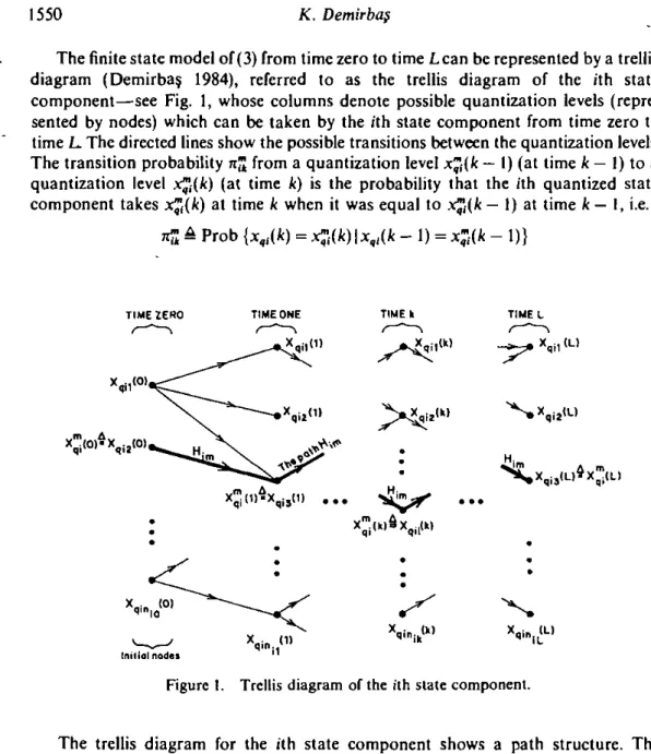
The finite state model of (3) from time zero to time Lcan be represented by a trellis diagram (Demirbav 1984). referred to as the trellis diagram of the ith state component-see Fig. 1, whose columns denote possible quantization levels (repre- sented by nodes) which can be taken by the ith state component from time zero to time L The directed lines show the possible transitions between the quantization levels. The transition probability n;; from a quantization level x;(k

-

I) (at time k - I) to a quantization level c i ( k ) (at time k ) is the probability that the ith quantized state component takes x;(k) at time k when it was equal to c i ( k - I) at time k

-

I, i.e.

rr;;P Prob {xqi(k) =$(k)Ix,,(k- I) =x;(k- I)}

Figure I. Trellis diagram or the ith slate component

The trellis diagram for the ith state component shows a path structure. The quantization levels along the paths of this trellis diagram can be taken by the ith state component from time zero to time L. Hence, the ith state component.smoothing finds a path through the trellis diagram so that the quantization levels along this path are the smoothed values of the ith state component from time zero to time L. Finding a path is a multiple composite hypothesis testing problem. The optimum testing rule that minimizes the overall error probability can be stated (Demirba? 1984) as

choose Hi, if

Mi

>

My

for all m # 1 _{( 5 )}

where H, is the lth path through the ith state component trellis diagram, and

My

is, by definition, the metric of the rnth path through the ith state component trellis diagram, which is defined by

Mulri-dimensional stare smoorhing by H,,) of the ith state component trellis diagram,

M(x;(O)) In { P r o b {xqi(0) = x;(O))}

which is, by definition, the metric of the initial node ( o r quantization level) x;(O), where In indicates the natural logarithm.

M[x;(k

-

I)

-

x;(k)] 4 In { d p [ z i ( k ) Ix,,(k) = x;(k)]}

which is, by definition, the metric of the branch connecting the node x;(k - 1) to the node .$(k), and

x Prob {l,(k) = I,,(k))

which is the conditional density function of the ith observation component, given that the ith quantized state component xqi(k) is equal to x;(k), where p[z,(k)lx,,(k) =

.~;(k). IJk) = I,,(!i)] is the conditional density function of z,(k), given that x,,(k) =

x;(k) and l,(k) = I,,(k), and l,,(k) is the ith possible value of l,(k).

The optimum decision rule o f ( 5 ) states that the quantization levels along the path with the greatest metric are the smoothed values of the ith state component from time zero to time L. For a given observation sequence ZL, if the inequality in (5)

becomes a n equality for more than one path, the quantization levels along any one of these paths can be chosen as the smoothed values of the ith state component from time zero to time L. This does not change the overall error probability. Hence, the smoothing of the ith state component finds the path with the greatest metric through the ith state component trellis diagram. T h e quantization levels along this path are the smoothed values of the ith state component. The path with the greatest metric can be found by the Viterbi decoding algorithm ( D e m i r b a ~ 1984). It follows from (3) that the

ith state component quantization levels at time k

+

1 are a function of the other state component estimates , ( k ) ,

....

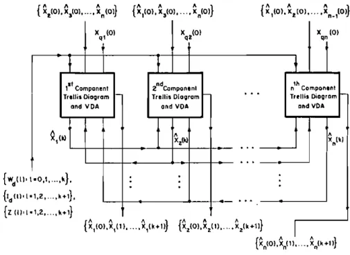
.<,-,(k), .t,+,(k), ..., .t,(k). Thus, these estimates are sequentially obtained by performing the smoothing of the n state components in parallel-see Fig. 2. where VDA represents the Viterbi decoding algorithm. The

recursive steps for the state smoothing can be stated a s follows: Srep k

(k

= 1, 2, ..., L)

Use the observation sequence Z k and the VDA lor each state component to estimate 11 state components from time zero to time k. This yields the smoothed values

{.i.,(O). .<;(I). ..., .i.,(k) : i = 1. 2,

...,

11) of the state components from time zero to time k. given the observation sequence Zk. The smoothed values of the state components at time k ( , ( k ) , .i.,(k).

...,

.<.(k)) are used to find the quantization levels at time k + I . This process at Step L yields the smoothed values o f t h e 11 state components from time

zero to time L.

At every step,a different smoothed value o f a statecomponent a t a given time can be obtained, since the path with the greatest metric can change whenever the trellis diagram is extended ( D e m i r b q 1984).

Assume that, without loss of generality, the numbers of possible values of the discrete initial state components and the discrete disturbance noise vector are component and time-invariant-i,e. ti;, 4 no, for i = 1, 2,

...,

11; and ntk 4 ni for :111 k. I t

can be shown (Demirba$ 1989) that the maximum number of quantization levels required for the implementation of the proposed smoothing scheme is nnomp'., whereas the number of maximum quantization levels for the implementation of the scheme presented by Demirba? and Leondes (1986) is n;mPL, where p and n are the dimensions of the disturbance noise and state vectors, respectively. Hence, this maximum number is a linear function of the dimension of the state vector for the proposed smoothing scheme, whereas it is an exponential function of the dimension of the state vector for the scheme presented by Demirba? and Leondes (1986).

( $ " l o ~ , ~ ~ l ~ : . . . . ~ ~ k + l ~ } Figure 2. Slate smoothing, component by component, in parallel.

4. Performance

The performance of the proposed smoothing scheme depends upon the perfor- mances of VDAs used in parallel to smooth the state components. Consider the ith state component smoothing with the VDA. The performance of this VDA can be quantified by a Gallager-type ensemble upper bound (Gallager 1965. Viterbi and Omura 1979), since the evaluation of the exact error probability or error probability bound for choosing the correct pa!h is complex.lt can be shown ( D e m i r b a ~ 1984) that such an ensemble bound is given by

with

where

Pi,

is the ensemble-averaged overall error probability for the ith stale component smoorhing;

X:

is the set of all possible quantization levels of the ith state component from time I to time L; qj(

.

) is an arbitrary probability density function on

Mulri-dimensional state smoothing 1553

X;;

p(zi(k)Ix) is the conditional density function of the ith observation component, given that the ith state component is equal to x; Mi is the number of possible paths through the trellis diagram ofthe ith state component;

nF

and

nr

are the minimum and maximum values of the occurrence probabilities of the possible values of the ith discrete initial state component xqi(0); and n:'" and

nr,

k

>

0, are the minimum and maximum values of the transition probabilities from time k - 1 to time k(in the trellis diagram of the ith state component), respectively.

The uniformly weighted ensemble bound with 6 = I-as the performance measure of the proposed smoothing scheme for the ith state component-is used since it is the easiest bound to evaluate (Demirbat 1984). 'Uniformly weighted' means that qi(.r) = IIN;, where N; is the number of elements in

XI.

Consider, as an example, the models whose ith components are given by

x,(k

+

I) =f,[k, x(k), w(k)] (the state model)

(7)

zi(!i) =gi[k, ..ri(k), I(k)]

+

hi[k, .ri(k), I(k)]ui(k) (the observation model) (8) where xi(0) and v,(k) are assumed to be gaussian noises with means mi, and 0 and variances R,, and R,,(k), respectively. h[k, rr,(k), I(k)] is a given (linear or non-linear) function such that [h,(k,xq,(k), I,,(k))12R,,(k) f-0, for all j, I and k. Substituting p[z,(k) Ix;(k) = x], 6 = 1, and q,(

.

) = (IIN;) into the bound in (6), and using the inequality

we obtain the bound

where

L[k, .r,, l,(k), x,, lj(k)]

A

C, exp

{

-

:

}

The bound of (9) is the one used as the performance measure of the proposed scheme for the ith statc component smoothing of the models (7) and (8).

Figure 3 (n). Actual and estimated values of the first slate' component .r,(k).

Figure 3 ( h l . Error variancesand bound for estimate solthe first state component .r,(k).

X I K + I ~ = X I S I . O . Z E X P I S I N I X I K > l . U I K l X ~ K . l l r X ~ K l l l + O . I E X P I C O S I X ~ n l I i ~ U l K l Z ~ K ~ ~ ~ ~ I ~ E X ? Z I C O S I I ( K I I I ~ X ~ ~ ~ ~ ~ ~ P I ~ ~ N I ~ ~ ~ ~ ~ ~ ~ ; ~ . ~ ~ I N I = I ~ . ~ ~ E X P I S ~ N I I I ~ I I I ~ X ~ ~ ~ ~ I ~ ~ ~ ~ N I I ~ ~ . I I ~ ~ ~ ~ ~ N u n . OF D I S C . FOR X I O I = 3 .11.1:3 V R R I X I O I 1 ~ 0 . 3 0 0 .VRRI l l .1 : = 0 . 2 0 0 E I X 1 0 1 1 = 1 . 5 0 0 . E l I l . > ) = I , 5 0 0

N u n . OF O I S C . FOR U;. 1 = 3 LEGEND V R R l U l . 1 1 = 3 . 0 0 0 a : n n L n a r V R R I V 1 . 1 1 : 1 . 0 0 0

+ :

ODSA GATE S I Z E = 0 . 2 5 0 A F E 6 - 0 2 0 6 9 3 7 E I

~ R E O P = C . I I 6 0 5 6 E I

Figure 5 (c). Absolute and rime-averaged absolute errors for estimates of the first state component x , ( k ) .

E l X l O l 1 : 1 . 7 0 0 . E l l 1 - 1 1 ~ 1 .ZOO

w m Nun. OF D I S C . FOR W i . 1 ~ 3 LEGEND Y R R I U I . 1 1 : 2 . 5 0 0 0 : n c r u n L

6% : K R L n R N

0 9 G A T E SIZE:O.%SO + : 0 0 5 R

Zrn

0

Figure S ( d ) . Actual and estimated values of the second

Multi-dinrensional stare smoothing 1563

5. Simulations

Computer simulations are used to evaluate the performance of the proposed smoothing scheme, and also to observe the divergence of the Kalman filter estimates, assuming zero interference. Many examples are simulated on the IBM 3081K mainframe computer. Examples with white gaussian noise and interference are considered. Random variables are approximated by the discrete random variables given by Demirba~ (1984). These random variables are also assumed to be time- invariant.

The simulation results of three examples are presented in Figs 3 (a)-5 ( n . At the top left-hand corner of each figure, the simulated models and statistics of random variables used are presented. Moreover, in the Figures E(B(

.

)), VAR (B(

.

)), and NUM. O F DISC. FOR B(

.

) denote the mean value and variance of the random variable B(

.

) and the number of possible values of the discrete random variable used to approximate the random variable B ( . ) ; ACTUAL, ODSA, and KALMAN represent the actual values and their estimates by the proposed smoothing scheme and the Kalman filter; AAEOP and AAEK represent the time averaged absolute errors for the proposed smoothing scheme and the Kalman filter: ER. COV. and BOUND indicate the error variances of the Kalman estimates and the performance bound- given by (9)-of the proposed smoothing scheme, respectively. One should note that this bound may become useless (i.e. a number greater than one), depending upon the models and gatesizes used, since some inequalities are used to drive the bound. Even if this bound is less than one, it does not exactly determine the performance of the proposed smoothing scheme, since i t is an ensemble bound on the overall error probability (Demirba? 1984).

The memory requirement for the implementation of the proposed smoothing scheme increases with the numbers of possible values of the discrete random variables and vectors o r smaller gate sizes used in the finite state models for state com- ponents. Moreover, this memory requirement increases exponentially with time. Hence, by choosing appropriate values for these numbers and gate sizes, one can obtain a desired estimation accuracy, using the available memory, for state smoothing.

The dynamic models, whose simulation results are presented in Figs 3 (a)-5 ( f ) are non-linear with non-linear interference. In other words, observation component models are non-linear functions of interference. The smoothed values of the state components, using the proposed smoothing scheme, closely follow the actual state component values, while the Kalman estimates assuming zero interference are far from the actual state component values. The proposed smoothing scheme is superior to the Kalman filter, which is incapable ofestimating the states ofdynamic models with non- linear interference. However, the implementation ofthe proposed smoothing scheme is more complex than the Kalman filter implementation, since the implementation of the VDA used for each state component smoothing is more complex.

6. Conclusions

The proposed estimation scheme is sub-optimum and applicable to state estim- ation for multi-dimensional dynamic systems with non-linear noise and interference; whereas the Kalman filter cannot, in general, be used to estimate the states of models with non-linear noise and interference. The implementation of the proposed scheme requires a linearly increasing memory; whereas the implementation of the scheme

1564 M u l t i - d i m e n s i o n a l stare smoothing

presented b y D e m i r b a ~ and Leondes (1986) requires a n exponentially increasing memory w i t h the dimension of the state vector. Moreover, b o t h o f these schemes require a n exponentially increasing m e m o r y w i t h time.

REFERENCES

DEMIRRAS. K.. 1984. Aduanres i n Conrroland Dynamic Sysrems. Vol. X X I (New York: Academic Press). pp. 175-295: 1989. In:. J. Systems Sci.. 20, 759.

DBMIRRA$. K.. and LIONOIS. C. T., 1985, Inr. J. Systems Sci., 16, 951: 1986, Ihid., 17, 251. FARINA, A., and PAR~INI, S., 1979, I.E.E.E. Trans. Aerosp. electron. Sysrem, 15, 555. FORNBY, G. D.. Jr.. 1974, in/ Conrrol. 25, 222.

GALLAGI:~. R. G.. 1965. I.E.E.E. Trans. I n ! Theory. ll. 3.

KAILATH~T.. 1968, I.E.E.E. Trans. aurom. Control. 13, 646; 1974. I.E.E.E. Trans. In/ Theory, 20,

146.

KALMAN, R. E., 1960. Trans. Am. Soc. mech. Engrs, Pt D, J . Bas. Engng, 82, 35.

KALMAN, R. E., and Bucv, B. C., 1961, Trans. Am. Soc. mech. Engrs.. Pf D, J . Bas. E n ~ n g , 83,95, MAKHOUL. . 1.. . 1975. Proc. Insr. elecr. elecrron. Eners.

..

. 63. 561. .

M e l x n . J. S., 1973. Auromarica. 9, 151.

MILLER. K. S.. and L~SKIW. D. M.. 1982. I.E.E.E. Trans. Aeroslr. elecrron. Svsrems. _. 18. 192. _.

MONZINCO.

R: A,. 1975. I.E.E.E. ~ r a n s . InJ Theory, 21. 271. .

NAHI. N. E.. 1969. I.E.E.E. Trans In! Theory. 15, 457.

SAC,. A. P.. and MELSA. J. L.. 1971, Esrimarion Theory wirh Applicalions ro Communicarions and Conlrol (New York: McGraw-Hill).

VAN TRECS, H. L.. 1968, Detection. Esrimarion and Modulation Theor)' (New York: Wiley). VITBRRI. A. J.. and OMURA. J. K.. 1979. Principles oJDigiral Communication and Coding (New