a thesis
submitted to the department of industrial engineering
and the institute of engineering and science
of bilkent university
in partial fulfillment of the requirements
for the degree of
master of science
By
Nurdan Ahat
Assist. Prof. Dr. Osman Alp (Advisor)
I certify that I have read this thesis and that in my opinion it is fully adequate, in scope and in quality, as a thesis for the degree of Master of Science.
Assist. Prof. Dr. Alper S¸en (Co–advisor)
I certify that I have read this thesis and that in my opinion it is fully adequate, in scope and in quality, as a thesis for the degree of Master of Science.
Prof. Dr. Nesim Erkip
I certify that I have read this thesis and that in my opinion it is fully adequate, in scope and in quality, as a thesis for the degree of Master of Science.
Assist. Prof. Dr. Ay¸se Kocabıyıko˘glu
Approved for the Institute of Engineering and Science:
Prof. Dr. Mehmet B. Baray Director of the Institute
PROTECTION
Nurdan AhatM.S. in Industrial Engineering
Supervisor: Assist. Prof. Dr. Osman Alp , Assist. Prof. Dr. Alper S¸en July, 2007
In an environment with declining sales prices, retailers (or any reseller) often face the risk of buying high and selling low. In order to limit their channel partners’ exposure to such risks and increase the availability of their products in the marketplace, suppliers often offer price protection. With price protection, a retailer is reimbursed with a percentage of the procurement cost declines, for the inventory that the retailer ordered within a given price protection age limit. We study the optimal inventory policy of the retailer under such price protection terms in a multi–period finite horizon setting with stochastic demand. We propose three different models for the treatment of unsatisfied demand. For the case of full backlogging, we show that the order–up–to type policies are optimal. In a numerical study, we study the behavior of the retailer and investigate the impact of price protection terms on the operational performance of the retailer and the supplier under a variety of settings.
Keywords: Inventory models, price protection, supply chain management, high– tech industry.
F˙IYAT KORUMASI ALTINDA C
¸ OK D ¨
ONEML˙I
ENVANTER MODELLER˙I
Nurdan Ahat
End¨ustri M¨uhendisli˘gi, Y¨uksek Lisans
Tez Y¨oneticisi: Yrd. Do¸c. Dr. Osman Alp, Yrd. Do¸c Dr. Alper S¸en Temmuz, 2007
Satı¸s fiyatlarının giderek d¨u¸st¨u˘g¨u bir ortamda, parakendeciler (veya herhangi bir satıcı) bir ¨ur¨un¨u y¨uksek fiyatla alıp daha d¨u¸s¨uk fiyatla satma riskiyle y¨uz y¨uzedir. Tedarik¸ciler, perakendecilerin bu t¨ur risklere maruz kalmasını engellemek ve ¨ur¨unlerin pazardaki hazır bulunabilirli˘gini arttırmak amacıyla, perakendecilere fiyat koruma stratejilerini sunmaktadır. Fiyat koruma stratejileri sayesinde, per-akendecinin sto˘gunda bulunan, belirli bir zaman aralı˘gında ısmarlanan envanterin fiyatında g¨ozlenen d¨u¸s¨u¸slerin belirli bir y¨uzdesi perakendeciye tedarik¸ci tarafından iade edilir. Bu tezde, tedarik¸cinin perakendeciye belirlenen terimlerle fiyat ko-ruma stratejisi uyguladı˘gı, ¸cok d¨onemli ve sonlu ufuklu bir ortamda rassal talep al-tinda perakendecinin en iyi envanter kontol politikasının belirlenmesi problemiyle ilgilenilmektedir. Zamanında kar¸sılanamayan talebi farklı ¸sekilde ele alan ¨u¸c model ¨onerilmektedir. Zamanında kar¸sılanamayan talebin tamamının daha sonra kar¸sılandı˘gı durumlarda seviye esaslı politikaların optimal oldu˘gu g¨osterilmi¸stir. Sayısal ¸calı¸smalar ile, ¸ce¸sitli ortamlarda perakendecinin davranı¸sı incelenmi¸s fiyat koruma politikası ko¸sullarının perakendecinin ve tedarik¸cinin operasyonel perfor-manslarına etkisi ara¸stırılmı¸stır.
Anahtar s¨ozc¨ukler : Envanter sistemleri, fiyat koruması, tedarik zinciri y¨onetimi, y¨uksek teknoloji end¨ustrisi.
I would like to express my deepest and most sincere gratitude to my advisors Assist. Prof. Dr. Osman Alp and Assist. Prof. Dr. Alper S¸en for their invaluable encouragement, trust, guidance and motivating support during my study. They have been supervising me with everlasting patience and interest. Their advices will be the closest, most important and valuable reference for my future.
I would like to express my special thanks to Prof. Dr. Nesim Erkip and Assist. Prof. Dr. Ay¸se Kocabıyıko˘glu for accepting to read and review this thesis and for their suggestions.
I am indebted to Prof. Dr. Mustafa Pınar for his invaluable advices and sincere talks and for sharing his enlightening vision with me about my future study and life. I would like to thank Assoc. Prof. Dr. Mustafa Akg¨ul for helping me in solving my computer related problems during my study. I also want to thank all the faculty members for devoting their time and knowledge to me.
I wish to thank my friends Berna C¸ elebi, Solmaz S¸irip, Keziban Akkaya and C¸ i˘gdem Akbulut for their existence at the other side of the phone ready to listen and talk to me when the taste of the loneliness started to cause an intolerable pain in my throat. I thank them all, for their luminous glances, closest conversations, and laughters and also, for listening to my delirious ideas with full understanding and tolerance and sharing their valuable thoughts with me.
I would like to thank Ay¸seg¨ul Altın for her interest and clemency when I was wriggling with an insufferable pain in my stomach on a Sunday morning in Ea331. I would also like to thank Evren K¨orpeo˘glu, ¨Onder Bulut and Ay¸seg¨ul Altın for their academic assistance and understanding, and being good friends to me.
I am grateful to my dear friends G¨ulay Samatlı, Esra Aybar, Mehmet Mustafa Tanrıkulu, Sıtkı G¨ulten, Emre Uzun, Muzaffer Mısırcı, Yahya Saleh, Hatice C¸ alık, Ali G¨okay Er¨on, K¨on¨ul Bayramo˘glu, and Tu˘g¸ce Akba¸s. I would like to thank all
the graduate students and Kaytarık¸cılar for being there.
I would like to thank T ¨UB˙ITAK for the financial support they have provided thus make this study happen.
Last but not the least, I would like to express my gratitude to my family for their trust and motivating attitudes. I especially thank to my brother, Mehmet Ahat, for his existence, everlasting love and morale support during my study. He was sometimes my mentor and only source of joy.
And I am grateful to all, who made me to find my way when I fell to the dark wells without any equipment and who made me remember that the stars are still shining and there is still hope...
1 Introduction 1
2 Literature Survey 5
3 Model 9
3.1 Standard Backorder Model . . . 13 3.2 Modified Backorder Model . . . 18 3.3 Lost Sales Model . . . 25
4 Numerical Study 27
4.1 Modified Backorder Model . . . 30 4.2 Lost Sales Model . . . 40
5 Conclusion 52
A Proof of Theorems 56
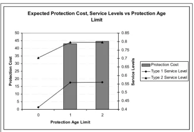
4.1 Expected Protection Cost for Supplier, Type 1 and Type 2 Service Levels of the Retailer vs Protection Age Limit (LD, Poisson(λ = 5),
α = 1, bi = 0.10c1, pi = ci+ 30) . . . 37
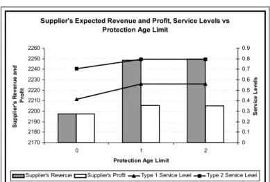
4.2 Expected Profit and Revenue for Supplier, Type 1 and Type 2 Service Levels vs Protection Age Limit(LD, Poisson(λ = 5), α = 1, bi = 0.10c1, pi = ci+ 30) . . . 38
4.3 Expected Protection Cost for Supplier, Type 1 and Type 2 Service Levels of the Retailer vs Protection Age Limit (LD, Poisson(λ = 5),
α = 1, bi = 0.30c1, pi = ci+ 30) . . . 39
4.4 Expected Revenue and Profit for Supplier, Type 1 and Type 2 Service Levels vs Protection Age Limit (LD, Poisson(λ = 5), α = 1, bi = 0.30c1, pi = ci+ 30) . . . 40
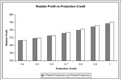
4.5 Expected Profit of the Retailer vs Protection Credit (LD, Poisson(λ = 5), bi = 0.10c1, pi = ci+ 30) . . . 41
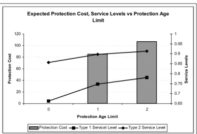
4.6 Expected Protection Cost for Supplier, Type 1 and Type 2 Ser-vice Levels of the Retailer vs Protection Age Limit (Linear Cost Decline, Demand Poisson(λ = 5), α = 1, bi = 0.10c1, hi = 0.10ci,
pi = ci+ 30) . . . 47
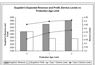
4.7 Expected Revenue and Profit for Supplier, Type 1 and Type 2 Service Levels of the Retailer vs Protection Age Limit (LD, Poisson(λ = 5), α = 1, bi = 0.10c1, hi = 0.10ci, pi = ci+ 30) . . . 48
4.8 Expected Protection Cost for Supplier, Type 1 and Type 2 Service Levels of the Retailer vs Protection Age Limit (LD, Poisson(λ = 5),
α = 1, bi = 0.30c1, hi = 0.10ci, pi = ci+ 30) . . . 49
4.9 Expected Revenue and Profit for Supplier, Type 1 and Type 2 Service Levels of the Retailer vs Protection Age Limit (LD,Poisson(λ = 5), α = 1, bi = 0.30c1, hi = 0.10ci, pi = ci+ 30) 50
4.10 Expected Profit of the Retailer vs Protection Credit (LD, Poisson(λ = 5), bi = 0.30c1, pi = ci+ 30) . . . 51
4.1 Problem Parameters . . . 28 4.2 Cost Decline Structures . . . 29 4.3 Percent Increase in Retailer Profit Under Different Price Protection
Policies (Poisson(λ = 5)) . . . . 31 4.4 Protection Cost and Percent Increase in Supplier’s Profit Under
Different Price Protection Policies (Poisson(λ = 5)) . . . . 33 4.5 Percent Increase in Retailer’s Service Levels Under Different Price
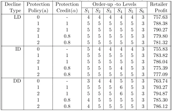
Protection Policies (Poisson(λ = 5)) . . . . 34 4.6 Retailer Profit and Order-up-to Levels Under Different Cost
De-cline Structures (Poisson(λ = 5),bi = 0.10c1, hi = 0.10ci, pi = ci+30) 35
4.7 Retailer Profit Under Different Distributions (LD, bi = 0.10c1,
pi = ci+ 30) . . . 41
4.8 Percent Increase in Retailer Profit Under Different Price Protection Policies (Poisson(λ = 5)) . . . . 42 4.9 Protection Cost and Percent Increase in Supplier’s Profit Under
Different Price Protection Policies (Poisson(λ = 5)) . . . . 43 4.10 Percent Increase in Retailer’s Service Levels Under Different Price
Protection Policies (Poisson(λ = 5)) . . . . 44 x
4.11 Retailer Profit and Order-up-to Levels Under Different Cost De-cline Structures (N = 6, Demand Poisson(λ = 5), LT = 0,bi =
0.10c1, hi = 0.10ci, pi = ci+ 30) . . . 46
4.12 Retailer Profit Under Different Distributions (LD, bi = 0.10c1,
Introduction
The high-tech products are characterized by their short life cycles and high de-mand variability. The suppliers of these products usually use direct and indirect channels to serve the customers. In the direct channel, the demand is satisfied by the supplier by means of catalogs, mail or internet sales, while in the indirect channel, the demand is satisfied through the distributors, retailers, partners, and etc.
In order to survive in the high-tech market, the supplier needs to offer new products to the market. This reduces the appeal and necessitates reductions in the price of the older products in both direct and indirect channels. Sometimes, suppliers also offer price reductions on older products prior to introduction of new products in order to clear the channel of older inventory. Frequent and significant price declines creates the risk of buying high and selling low for the participants of the indirect channel. Therefore, the indirect channel has less incentive for buying the products at the beginning of their life cycle; this leads to reduced availability of new products in the market. In order to limit the indirect channel’s exposure to the risk of buying high and selling low and increase the availability of the product in the market, the manufacturers often offer return or price protection policies.
With price protection, if the supplier reduces the list price of an item, he 1
reimburses the channel participants the difference between what they have paid and the current price for all inventories they have ordered but not yet sold. In some cases, the supplier may impose an age limit on inventories that the channel partners can claim reimbursements, i.e. the protection is valid for only those items that are ordered within a certain period of time. Also, he may impose a limit on the magnitude of the price protection credit, i.e. only a certain percentage of the price change is credited.
Price protection enables the retailer to maintain its profit margin regardless of the price offered by the supplier and reduces the cost of carrying inventory for the retailer. While more price protection is always better for the retailer, the supplier needs to trade off between increased availability of its products in the market and the “cost” of price protection. Price protection can be costly for the supplier in two ways. First type of costs are concrete: with every price decline the manufacturer reimburses the difference between the paid price and current price for the inventory held but not sold in the indirect channel. The second type of costs can be caused by excessive amount of inventory that is carried by the indirect channel due to price protection. This may result in supplier having difficulty in introducing new products to the market as its pipeline is full of older inventory. In addition, price protection limits the supplier’s control in tactical pricing. This may be true not only in indirect channel but also in direct channel, as the industry evidence shows that the retail prices in traditional channels are usually same as the prices in supplier’s direct channel (See [7] for a few examples). When considering a price drop, the supplier needs to take into account the amount of channel inventory for which needed to be reimbursed under the price protection policy (this is in addition to demand elasticity, competition, amount of component inventory and all other factors that impact a pricing decision). Payments to the channel due to price protection may potentially erase all the benefits that the manufacturer is seeking from a price drop. If not managed properly, price protection costs may add up to significant levels.
Many companies in the high–tech industry adopted price protection policies for their indirect channel. Examples include Hewlett Packard, Apple, Compaq, IBM, Seagate, and Maxtor which offer various price protection and return terms in
their contracts to ensure availability of their products in the market ([2], [15], [16], [11], [13]). Hewlett Packard (HP) developed a metric called inventory-driven costs which identifies price protection costs to be one of the major hidden components of cost of holding inventory [2]. Many companies have frequent adjustments to their price protection policies in an effort to strike a balance between keeping their indirect customers happy (hence, the availability of their products in retail) and reducing their price protection costs. Various articles report changes to price protection policies by major companies. Compaq set an age limit of 15 days on price protection [16]. HP announced a reduction in price protection for personal computers [1]. Apple first had set an age limit of 30 days on price protection, but then had to reinstate the full protection after pressure from its indirect customers [15].
In order for the supplier to evaluate any price protection policy alternative, the supplier needs to have a good understanding of how the indirect channel reacts to price changes in the existence of a price protection mechanism. Pre-requisite to this is understanding channel behavior under fixed prices and a given price protection mechanism. In this thesis, we study the inventory problem of an indirect channel partner (e.g. a retailer) who faces decreasing prices and is offered a price protection policy in a multi–period setting. The retailer’s problem is modeled under the assumption of standard backordering, modified backordering (which allows the loyal customer to buy the item from the newer price), and lost sales. Also, the cost of the price protection policy to the supplier is determined assuming that the retailer is rational and operating with an optimal decision rule.
The organization of the thesis is as follows:
In Chapter 2, we provide a review of the literature in the price protection mechanisms and supply chain coordination.
In Chapter 3, we model the ordering problem of the retailer for three different assumptions for the case of shortages. The first of these is the Standard Backorder Model (SBM), in which the retailer can satisfy the demand later. The customer is charged with the price that is used when the customer first appears. The retailer incurs a backorder cost for each item satisfied with a delay. The second
application for the excess demand is the Modified Backorder Model (MBM), in which the retailer satisfies the demand after a while, incurs a backorder cost for each item backordered as in Standard Backorder Model. However this time the owner of the backordered items is charged with the price that is effective when the customer demand is satisfied. The third application for the excess demand is the Lost Sales Model (LSM). In this model excess demand is completely lost. The retailer incurs a shortage cost for each demand lost. The optimal decision rule for the retailer when the supplier offers price protection is determined to be order-up-to type policy for the SBM and MBM.
In Chapter 4, a numerical study with different problem parameters is con-ducted under MBM and LSM. The optimal decision rule of the retailer is verified to be order-up-to type policy for the MBM and it is observed that the optimal ordering policy for the retailer is also order-up-to type in LSM. The cost paid for the price protection policy by the supplier and the service levels of the retailer is determined when the retailer behaves rationally and applies the optimal order-up-to policy for ordering decisions. The simulation results indicate that the service levels of the retailer increases by introducing price protection. The increment in the service levels decreases as the age of the unsold inventory protected by the supplier increases.
In Chapter 5, we summarize our results and contributions to the literature, and suggest future research directions.
Literature Survey
In this chapter we study the literature that is closely related to the problem under concern. We begin with the seminal work of Clark and Scarf [3] who model multi-period stochastic inventory problems with dynamic programming. In their paper, a single installation multi-period inventory problem whose objective is to minimize the cost over the horizon is modeled. A positive lead time for the replenishment of the orders is assumed. The state vector at any period is defined as the outstanding orders plus the inventory level of the retailer. A purchasing decision is made at the retailer level after the orders that are placed lead time periods ago are received and they also consider the holding and the shortage costs of the retailer. They assume that the excess demand is backordered. The authors discuss that the optimal decision rule for the retailer is order-up-to type.
In an other stream of research, there are articles which attempt to model the price changes in the multi-period stochastic inventory environments. Gavirneni [6] models the periodic review inventory problem where the product prices change in a Markovian fashion from one period to the next. The product prices decline from one period to the other where the decline structure is defined in a probability transition matrix which is assumed to be regenerative and communicative. It is assumed that there are no set up costs, capacity restrictions, nor lead times. The unsatisfied demand is lost and a linear holding cost for extra inventory on hand is incurred. Under all these assumptions, the author shows that the optimal
ordering policy of the retailer is a base stock policy in a single period, finite horizon or discounted infinite horizon problems. Also [4] models the single item, periodic review inventory problem when the demand is stochastic but depends on the the selling prices of the item. They characterize the structure of the optimal pricing and inventory strategy and develop a value iteration method for calculating the optimal strategies. In [5], they consider multiple retailers in the same setting when the demand distribution at each retailer can vary. In the paper, an approximate model for the problem is developed and combined pricing, ordering and allocation strategies are provided.
Another paper that models the price decline of the product in a multi-period environment is by Wang [14]. A single item, single location inventory system that is reviewed periodically and that faces a stochastic demand is considered. The demands of the successive periods are independent and identically distributed. The acquisition cost of the item in the successive periods is modeled as decreasing random variables. Therefore, the selling price of the item decreases in the unit acquisition cost as well. Two pricing fashions are handled in the paper: The retailer price is determined by adding a fixed percent mark-up or fixed amount mark-up to the acquisition cost of the item. It is shown that the order-up-to type policy is optimal for the backorder and the lost sales models.
Price protection problem is first introduced by Lee et al. [8]. They consider a 2-period problem in which the supplier offers the retailer a protection policy. They assume that the manufacturer has no capacity restrictions, the set-up cost is negligible, and the excess demand is lost. They consider two cases for purchasing action of the retailer: the retailer may have a single buying or two buying oppor-tunity. In the single buying opportunity case, it is shown that a properly chosen protection credit coordinates the channel and guarantees a win-win situation. It is shown that the optimal order quantity of the retailer without protection policy is strictly less than the optimal order quantity of the integrated channel with price protection policy.
In the two buying opportunity case, it is shown that the order-up-to type policy is optimal and the order-up-to level of the retailer stays the same with
price protection or without price protection in the second period. However, the optimal order quantity of the first period is larger when the supplier offers the retailer a price protection policy. Since the order-up-to level does not change in the second period and the demand is coming from the same distribution in both cases, optimal order quantity in the second period is non-increasing. Therefore, the overall impact of the price protection policy on the retailer’s situation is that the total order quantity throughout the horizon increases or stays the same. If the acquisition cost of the item is set in two periods, price protection does not guarantee channel coordination. If the supplier is allowed to adjust the acquisition cost and the protection rebate simultaneously, the assumption that the acquisition cost has to be larger than the manufacturing cost is relaxed, and the acquisition cost of the product is announced at the beginning of the first period, then the channel coordination is restored.
Our model extends the problem that is described in a 2-period environment by Lee et al. [8]. However, we do not examine the channel coordination nor the supplier’s problem. We model the retailer’s problem in a multi-period environ-ment and analyze the optimal decision rule in the existence of the price protection policy. We also examine the effect of the protection policies to the performance metrics of the players.
Taylor [12] explores the policy combinations that are channel coordinating and implementable that increase the profit margins of the players in the supply chain when compared with the decentralized case. Three channel policies which are commonly adopted in declining price environments for channel coordination are handled. These policies are: price protection (P), end of life returns (E) and mid-life returns (M). The problem is modeled in a 2-period setting with two parties where the demand observed in each period is independent. The stock out and holding costs are negligible and all the exogenous variables are assumed to be known by the players at the beginning of the first period. It is concluded that under the declining price environments, EM achieves channel coordination but does not guarantee a win-win outcome. In the use of PEM, both channel coordination and win-win situation is attained. It is shown that if the retail prices are constant over time, both channel coordination and a win-win situation
is achieved by the implementation of EM.
Later, Lu et al. [10] adds rebate (R) policy to E and M which can be utilized instead of P. In R, the supplier specifies a credit which is obtained by the retailer for each unit sold after an acquisition cost decline. The effectiveness of these policies, channel coordination, win-win situation conditions are explored. Lu et al. [10] include the stock-out and holding costs to the model. Similar to the environment of Lee et al. [8], the retailer may have a single buying opportunity or a two buying opportunity. In the single buying opportunity, PEM or REM guarantees a win-win outcome. The conditions under which ME coordinates the channel are determined and discussed. In the two buying opportunity case, it is shown that win-win policy may not exist, and that in the absence of stock-out costs in the first period, PEM always leads to a win-win stock-outcome. The major contribution is that detailed procedures for determining the win-win policy parameters under the assumption that the acquisition cost never exceeds the retailer price are proposed.
Liu [9] explores the effects of the price protection policy on the channel per-formance in a multi-period environment with deterministic demand structure. In the paper, the age limit of the price protection policy is set to one and the supplier offers full protection to the retailer. The demand is known to the retailer and the supplier and it is decreasing in the selling price. The procurement lead time is negligible and the supplier is ample. Also it is assumed that the market size is non-increasing over time. The performance of the supply chain is compared with the case where there is no protection and supplier uses price-only contract in which the supplier announces the price and the retailer determines the order quantity and selling price in order to satisfy the demand. The impact of the price protection policy to the pricing decisions of the players in the supply chain is studied in the paper. In our study, the effect of the price protection policy to the ordering decision of the retailer and the supplier’s performance metrics are ex-plored. Also the problem is modeled in a stochastic environment in decentralized supply chain.
Model
We consider an inventory control problem of a retailer under a single item, finite planning horizon setting where the supplier with an ample capacity offers a price protection policy to the retailer. The supplier can impose a limit on the price protection credit in the sense that up to a certain portion of the inventory is protected. The supplier sets a certain age limit for the unsold inventory at the retailer to be reimbursed when a price decline decision is made by the supplier. The credit and the age limits do not change throughout the horizon. We consider three different models to treat the excess demand at the retailer: Standard Back-order Model (SBM), Modified BackBack-order Model (MBM), and Lost Sales Model (LSM). The set-up cost is assumed to be zero so that the retailer is not charged any additional amount for placing an order to the supplier. The retailer may be subject to a procurement lead time where the items ordered are received after a period of lead time. The holding and shortage costs are incurred after observing the demand and the acquisition cost is incurred at the beginning of the period. In SBM and MBM any excess demand is backordered with a cost incurred per item per period, whereas in LSM excess demand is lost with a cost incurred for each unit lost. In SBM and MBM, the selling price charged to a backordered customer is different. In SBM, at the time of the demand realization, the customers whose demands are backordered pay the current selling price of the item but receive their demand when the retailer’s stocks become available. Since the selling price
of the item may drop in time in our problem environment, the price that has already been charged to a backordered customer may be higher than the price of the item at the time of the backorder clearance. The difference between the selling prices can be interpreted as the reservation cost that is incurred by the backordered customer for the motivation of the retailer to order more and keep the item in his stocks. In MBM, the backordered customers pay the selling price of the item that is effective when they receive their demand from the retailer. In LSM, the excess demand is lost. The retailer incurs a shortage cost and the potential profit from this customer is also lost.
The sequence of the events at any period at the retailer is as follows:
1. At the end of a period, the inventory level is reviewed and determined. If the inventory level is less than zero, shortage costs are incurred. If the inventory level is positive, then the excess inventory is carried to the next period by incurring a holding cost.
2. At the beginning of the next period, if there is a reduction is the acquisition costs and there exists protected inventory at the retailer then the supplier reimburses the protected quantity.
3. An order is placed to by the retailer based on the current inventory position (i.e. inventory level plus the orders placed but not received yet). The acquisition costs are incurred.
4. The order which was placed lead time periods ago is received and the in-ventory level is updated.
5. Demand is observed.
At the end of the planning horizon, if there is positive inventory left at the retailer and in case a decline in the purchasing price, the unsold inventory under protection is reimbursed by the supplier in all models. In SBM and MBM, the excess demand at the last period of the horizon is satisfied by the retailer by means of market clearance obligation of the retailer. However in LSM, it is lost.
Before detailing the description of the model, we provide the notation that is used throughout the thesis:
N = Number of periods,
a = Protection age limit of the price protection policy, α = Price protection credit, 0 < α ≤ 1,
l = Procurement lead time between the retailer and the supplier, Wk = Random variable denoting the demand during the kth period,
F (wk) = The distribution function of the demand, Wk,
f (wk) = The probability distribution function of the demand, Wk,
Dk = Average demand at the kth period,
γ = Discount factor,
bk = Unit shortage cost in period k,
hk = Unit holding cost in period k,
ck = Unit acqusition cost of the item in period k,
∆ck = ck− ck−1,
pk = Unit selling price of the item in period kth,
∆pk = pk− pk−1,
qk = Order placed by the retailer at the beginning of the kth period,
xk = Inventory level at the beginning of the kth period after,
the replenishment ˜
xk = State of the system at the beginning of the kth period including the
starting inevntory level, xk, and the orders placed in the past a periods,
Jk(˜xk) = Minimum cost incurred in periods k, k + 1, ..., N in SBM, when
the system state is ˜xk,
Rk(˜xk) = Maximum profit obtained in periods k, k + 1, ..., N in MBM and
LSM, when the system state is ˜xk.
At the beginning of period k, we assume that ck’s and pk’s are known by the
channel partners, pk> ck, and a ≥ l
In Sections 3.1, 3.2 and 3.3, we present Dynamic Programming (DP) models for SBM, MBM and LSM respectively. Initially, we provide the common arguments that are used in the models. In order to construct a DP model, we need to define the state vector, ˜xk, that contains the state variables. The state variables of the
problem at any period are the orders that the retailer placed in the last a periods and the on hand inventory at the beginning of the period. The state vector for the price protection problem is the following:
˜ xk = ³ xk, qk−a, qk−a+1, ..., qk−l, qk−l+1...qk−1 ´ .
The next step is determining the evolution equation that is used to determine the following state vector given the current state vector. The state vector ˜xk
at period k, evolves into the following state vector at period k + 1 at SBM and MBM. ˜ xk+1 = ³ xk+ qk−l− wk, qk−a+1, qk−a+2, ..., qk−l, qk−l+1, ..., qk−1, qk ´ . There is a small change in the evolution equation in the LSM which is discussed in Section 3.3.
Let vk = qk−l+1+ ... + qk−1 be the outstanding orders at the kth period after
receiving the order placed l periods ago. Thus, the total protected amount in period k, ηk, is given by:
ηk= α(qk−a+ ... + qk−l+ vk) if xk− qk−a− ... − qk−l− vk ≥ 0 α(xk+ vk) if xk− qk−a− ... − qk−l− vk < 0 0 if xk+ vk ≤ 0
If xk− qk−a− ... − qk−l− vk≥ 0, the retailer has still items unsold in his inventory
that are purchased a periods ago. The protected quantity is given by: α(qk−a+
... + qk−l+ vk) which is the maximum possible inventory under protection.
If xk− qk−a− ... − qk−l− vk< 0, the retailer has already started to sell the items
that are purchased a periods ago and in this case the inventory under protection is: α(xk+ vk).
If xk+ vk≤ 0, there are no unsold items in the retailer’s stocks or in the pipeline
and the retailer has already sold all the inventory to the customers and therefore the inventory under protection is zero.
Therefore, total number of the protected items in the kth period is given by
ηk = α min{qk−a+ ... + qk−l+ vk, xk+ vk}+.
3.1
Standard Backorder Model
In SBM, since the price charged to the backordered customers is always the effective price at the time of demand realization. The ordering policy employed does not have any impact on the total revenue generated from the customers. Hence we can model this environment with a cost minimization objective. Let Jk(˜xk) be the minimum cost incurred in period k when the system state is ˜xk,
then SBM-DP: JN +l+1(˜xN +l+1) = α∆cN +l+1min{qN +l+1−a+ ... + qN, xN +l+1}+ + cN +l+1max(−xN +l+1, 0) Jk(˜xk) = min qk=0 {ckqk+ L(xk+ qk−l) + α(ck− ck−1) min{qk−a+ ... + qk−l+ vk, xk+ vk}+ + γEWk(Jk+1(˜xk+1))} ∀ k = N + 1, ..., N + l Jk(˜xk) = min qk≥0 {ckqk+ L(xk+ qk−l) + α(ck− ck−1) min{qk−a+ ... + qk−l+ vk, xk+ vk}+ + γEWk(Jk+1(˜xk+1))} ∀ k = 1, 2, ..., N, FWk(0) = 1 ∀ k = 1, ..., l where L(y) = hk Ry 0(y − wk)dF (wk) + bk R∞ y (wk− y)dF (wk)
In the above formulation if k − l < 0, qk−l ≡ 0. The retailer stops ordering
at the Nth period but the retailer continues to observe demand in periods N +
1, N + 2, ..., N + l. Hence, even though the end of the planning horizon is N, the business transactions finish at the end of period (N + l). We assume that the unit acquisition cost is the same throughout the periods N + 1, N + 2, ..., N + l so that cN +1= ck ∀ k = N + 1, ..., N + l.
If the procurement lead time is zero and the protection age limit is one, the DP is written as follows: SBM-DP-1: JN +1(˜xN +1) = α∆cN +1min(xN +1, qN)++ cN +1max(−xN +1, 0) Jk(˜xk) = min qk≥0 {ckqk+ L(xk+ qk) + α∆ckmin{xk, qk−l}+ + γEWk(Jk+1(˜xk+1))} ∀ k = 1, 2, ..., N.
In Theorem 1, for a = 1 and l = 0 we show that SBM-DP-1 can be transformed into another DP formulation, where the inventory level attained after ordering, yk,
is the only decision variable, the optimal of this variable is found by minimizing a convex function which is independent of the state variables and hence an order-up-to type policy is the optimal ordering policy of the retailer under the condition that the total holding and backorder costs at any period is greater than the protection credit paid by the supplier to the retailer (i.e. hk+ bk+ α∆ck+1 ≥ 0).
According to the the order-up-to type policy, the retailer is supposed to increase the inventory level to an optimal order-up-to point that is determined by the minimum of a convex function, if the inventory level of the retailer is less than the optimal-order-up-to point. Otherwise, the retailer does not order.
qk∗ =
(
y∗
k− xk if xk < yk∗
0 if xk ≥ y∗k
Also, optimal order-up-to level in the last period is given by
y∗ N = F−1 µ bN − cN + γcN +1 hN + bN + γα∆cN +1+ γcN +1 ¶ ,
if total holding, backorder and selling price of the item is greater than the protec-tion credit offered by the supplier in the last period (i.e. hN + bN + γα∆cN +1+
γcN +1 ≥ 0).
Theorem 1 For a = 1, l = 0, if hk+ bk+ α∆ck+1 ≥ 0 ∀ k = 1, 2, ..., N − 1, and
(i) SBM-DP-1 is equivalent to the following problem: JN +1(˜xN +1) = α∆cN +1min(xN +1, qN)++ cN +1max(−xN +1, 0) Jk(˜xk) = min yk≥xk {Gk(yk)} − γα∆ck+1Φ(xk) + α∆ckmin(xk, qk−1)+− ckxk + Ãi=N −1 X i=k
γi+1−k¡ci+1Di+ Gi+1(yi+1∗ )
¢! + γN +1−kcN +1DN ∀ k = 1, 2, ..., N where Gk(yk) = (ck− γck+1)yk+ L(yk) + γ Z yk−y∗ k+1 0 Gk+1(yk− wk)dF (wk) − γGk+1(yk+1∗ )F (yk− yk+1∗ ) − γ2α∆ck+2 Z ∞ 0 Φ(yk− wk)dF (wk) + γα∆ck+1Φ(yk)∀ k = 1, 2, ..., N − 1. GN(yN) = (cN − γcN +1)yN + L(yN) + γΦ(yN)(α∆cN +1+ cN +1) f or k = N. Φ(y) =R0yF (t)dt, GN +1(yN +1) = 0, and y∗ k = argminyk{Gk(yk)} ∀ k = 1, 2, ..., N.
(ii) Jk(˜xk) is convex in ˜xk and Gk(yk) is convex in yk ∀ k = 1, 2, ..., N .
(iii) Optimal ordering policy of the retailer is an order-up-to type policy that
states if the inventory level of the retailer is less than y∗
k, the order quantity bring
the inventory level to yk∗, otherwise do not order. The following summarizes the
order-up-to type policy,
q∗ k = ( y∗ k− xk if xk < y∗k 0 if xk ≥ yk∗
(iv) Optimal order-up-to level of the last period is:
y∗ N = F−1 µ bN + γcN +1− cN hN + bN + γα∆cN +1+ γcN +1 ¶ . ¤
If the procurement lead time is zero and the protection age limit is 2, the DP can be written as follows: SBM-DP-2: JN +1(˜xN +1) = α∆cN +1min(xN +1, qN + qN −1)++ cN +1max(−xN +1, 0) Jk(˜xk) = min qk≥0 {ckqk+ L(xk+ qk) + α∆ckmin{xk, qk−1+ qk−2}+ + γEWk(Jk+1(˜xk+1))} ∀ k = 1, 2, ..., N
In Theorem 2, We extend the results for Theorem 1 to a = 2 when l = 0.
Theorem 2 For a = 2 , l = 0, if hk+ bk+ γα∆ck+1 ≥ 0 ∀ k = 1, 2, ..., N − 1,
and if k = N hN + bN + γα∆cN +1+ γcN +1≥ 0,
(i) SBM-DP-2 is equivalent to the following problem:
JN +1(˜xN +1) = α∆cN +1min(xN +1, qN + qN −1)++ cN +1max(−xN +1, 0) JN(˜xN) = min yN≥xN {GN(yN)} − γα∆cN +1Φ(xN − qN −1) + γcN +1DN + α∆cNmin(xN, qN −1+ qN −2)+− cNxN. where GN(yN) = (cN − γcN +1)yN + L(yN) + γΦ(yN)(α∆cN +1+ cN +1). Jk(˜xk) = min yk≥xk {Gk(yk)} − γ2α∆ck+2 Z ∞ 0 Φ(xk− wk)dF (wk) − γα∆ck+1Φ(xk− qk−1) + α∆ckmin(xk, qk−2+ qk−1)+− ckxk + Ãi=N −1 X i=k
γi+1−k¡ci+1Di+ Gi+1(y∗i+1)
¢! + γN +1−kcN +1DN ∀ k = 1, 2, ..., N − 1. Gk(yk) = (ck− γck+1)yk+ L(yk) + γ Z yk−y∗ k+1 0 Gk+1(yk− wk)dF (wk) − γGk+1(yk+1∗ )F (yk− yk+1∗ ) − γ3α∆c k+3 Z ∞ 0 Z ∞ 0 Φ(yk− wk+1− wk)dF (wk+1)dF (wk) + γα∆ck+1Φ(yk) if k = 1, 2, ..., N − 2,
GN −1(yN −1) = (cN −1− γcN)yN −1+ L(yN −1) + γ Z yN −1−y∗ N 0 GN(yN −1− wN −1)dF (wN −1) − γGN(yN∗ )F (yN −1− yN∗) + γα∆cNΦ(yN −1) if k = N − 1. Φ(y) =R0yF (t)dt, GN +1(yN +1) = 0, yN +1∗ = 0, y∗ k = argminyk{Gk(yk)} ∀ k = 1, 2, ..., N.
(ii) Jk(˜xk) is convex in ˜xk and Gk(yk) is convex in yk ∀ k = 1, 2, ..., N .
(iii) Optimal ordering policy of the retailer is an order-up-to type policy. That is,
q∗k =
(
y∗
k− xk if xk < y∗k
0 if xk ≥ yk∗
(iv)The order-up-to level of the last period is
y∗ N = F−1 µ bN − cN + γcN +1 hN + bN + γα∆cN +1+ γcN +1 ¶ . ¤
In Theorems 1 and 2, we prove that the base stock policy is optimal. According to the base stock policy, the retailer is supposed to increase the inventory level to an optimal order-up-to point that is determined by the minimum of a convex function, if the inventory level of the retailer is less than the optimal-order-up-to point. Otherwise, the retailer does not order. Also, we observe that the order-up-to levels of the models with single protection period and double protection period are the same for the last period. This can be the consequence of allowing backorders. In this case no demand is lost, some of them are satisfied on time and some of them are satisfied with a little delay and a backorder cost. Thus the market share remains the same for the retailer. In this setting increasing the protection period does not affect the ordering amounts but the total costs. Also, we observe the convexity conditions for the single and double period protection is the same. In both cases, the convexity is preserved at any intermediate period if the total holding and backorder costs of the retailer is higher than the protection credit offered by the supplier. That is if the protection credit offered by the supplier is higher than the total holding and backorder costs incurred by the
retailer, then the retailer will simply prefer no action with the customers and the model will not be valid. Also, for the last period in order to preserve the convexity, total holding, backorder and discounted acquisition cost of the item for the ending period (N + 1) should be grater or equal to the discounted protection credit offered by the supplier for the ending period (N +1). Otherwise, the retailer would choose no action with the customers and the model would be meaningless. SBM is applicable for the products whose demand rate is high but manu-facturing rate is low. Therefore, the customers who cannot find the product in the market becomes willing to pay the reservation cost and wait for the product to become available in the retailer’s stocks. Reservation cost can be considered as the difference in the selling price of the product between the period that the demand is observed and the period that it is satisfied. Since the acquisition cost declines in time, reservation cost is non-negative. Modeling the environments that includes the products like computer game consoles (e.g. Sony Play Station) using SBM would be more meaningful. Since these products are manufactured in limited quantity and the demand of the item depend on the popularity of the product among the customers. Also, there is a decline in the acquisition cost of the product, since the newer ones are prepared for the market. Therefore, the customers are willing to pay the reservation cost for the product that they want to have.
3.2
Modified Backorder Model
In MBM, the selling price charged to a customer whose demand is backordered is the price that is effective at the time of the backorder clearance. The total expected profit obtained in such environments depends on the operating policies employed, since the selling price charged to a backordered customer may drop in the mean time until the backorder is cleared. Hence, problem in this setting should be modeled with a profit maximization objective. The following formula-tion is valid for the profit to go funcformula-tion in the kth period:
MBM-DP: RN +l+1(˜xN +l+1) = −α∆cN +1min{qN +l+1−a+ ...qN, xN +l+1}+ + (pN +1− cN +1) max(−xN +l+1, 0) Rk(˜xk) = max qk=0 {−ckqk+ pk(max(0, min(0, xk+ qk−l) − xk) + EWk{min(xk+ qk−l, Wk) +}¢ − L(xk+ qk−l) − α(ck− ck−l) min{qk−a+ ... + qk−l−1+ vk, xk+ vk}+ + γEWk(Rk+1(˜xk+1))} ∀ k = N + 1, ..., N + l, Rk(˜xk) = max qk≥0 {−ckqk+ pk(max(0, min(0, xk+ qk−l) − xk) + EWk{min(xk+ qk−l, Wk) +}¢ − L(xk+ qk−l) − α(ck− ck−l) min{qk−a+ ... + qk−l−1+ vk, xk+ vk}+ + γEWk(Rk+1(˜xk+1))} ∀ k = 1, 2, ..., N, where L(y) = hk Z y 0 (y − wk)dF (wk) + bk Z ∞ y (wk− y)dF (wk) FWk(0) = 1 ∀ k = 1, ..., l.
Let Ukbe the money collected by the retailer at the end of the kthperiod provided
that the beginning net inventory level of the retailer is xk, the inventory delivered
to the retailer’s stocks at the beginning of the kth period is q
k−l, and the order
placed by the retailer after the replenishment is qk. Then we have
Uk = pkqk−l if xk+ qk−l < 0 and xk < 0 −pkxk+ EWk(min(xk+ qk−l, Wk)) if xk+ qk−l ≥ 0 and xk< 0 pkEWk(min(xk+ qk−l, Wk)) if xk+ qk−l ≥ 0 and xk≥ 0
This is exactly obtained by the following expression
pk
¡
max(0, min(0, xk+ qk−l) − xk) + EWk{min(xk+ qk−l, Wk) +}¢.
For l = 0 and a = 1 we have, MBM-DP-1: RN +1(˜xN +1) = −α∆cN +1min(xN +1, qN)++ (pN +1− cN +1) max(−xN +1, 0) Rk(˜xk) = max qk≥0 {−ckqk+ pk(max(0, min(0, xk+ qk) − xk) + EWk{min(xk+ qk, Wk) +}¢ − L(xk+ qk) − α∆ckmin(xk, qk−1)++ γEWk(Rk+1(˜xk+1))} ∀ k = 1, 2, ..., N
In Theorem 3, for a = 2 and l = 0 we show that MBM-DP-1 can be transformed into another DP formulation, where the inventory level attained after ordering, yk,
is the only decision variable, the optimal of this variable is found by maximizing a concave function which is independent of the state variables and hence order-up-to type policy is optimal ordering policy for the retailer under the condition that the total holding, backorder and selling price of the item in the k0th period is higher
than the discounted total of the protection credit that will be delivered and the selling price of the item in the next period (i.e. (−pk+γpk+1−γα∆ck+1−hk−bk) ≤
0). According to the order-up-to type policy, the retailer is supposed to increase the inventory level to an optimal order-up-to point if the inventory level of the retailer is less than this point. Otherwise, the retailer does not order. More formally, the following is valid for the order-up-to type policy:
q∗ k = ( y∗ k− xk if xk < yk∗ 0 if xk ≥ y∗k
Also, optimal order-up-to level in the last period is given by
yN∗ = F−1 µ bN + cN − pN − γcN +1+ γpN +1 −pN − γα∆cN +1+ γpN +1− γcN +1− hN − bN ¶ ,
if the total holding, backorder and selling price of the item is higher than the discounted total of the protection credit that will be paid to the retailer at the end of the horizon and the profit margin of the retailer that will be obtained from
selling a single item to a customer (i.e. (−pN+ γpN +1− γα∆cN +1− γcN +1− hN−
bN) ≤ 0).
Theorem 3 For a = 1, l = 0, if (−pk + γpk+1 − γα∆ck+1 − hk − bk) ≤ 0 ∀
k = 1, 2, ..., N − 1, and if (−pN+ γpN +1− γα∆cN +1− γcN +1− hN− bN) ≤ 0 then,
(i)assuming that yk= xk+qkand yk > 0, therefore max(0, min(0, xk+qk)−xk) =
max(−xk, 0)
MBM-DP-1 is equivalent to the following problem:
RN(˜xN) = max yN≥xN {GN(yN)} + γα∆cN +1Φ(xN) + γ(pN +1− cN +1)DN + pNmax(−xN, 0) + cNxN − α∆cNmin(xN, qN −1)+ where GN(yN) = yN(−cN + pN + γcN +1− γpN +1) + Φ(yN)(−pN − γα∆cN +1+ γpN +1− γcN +1) − L(yN), Rk(˜xk) = max yk≥xk {Gk(yk)} + γα∆ck+1Φ(xk) + pkmax(−xk, 0) − α∆ckmin(xk, qk−1)+− ckxk + Ã i=N −1X i=k γi+1−k¡(p
i+1− ci+1)Di+ Gi+1(yi+1∗ )
¢! + γN +1−kc N +1DN ∀ k = 1, 2, ..., N − 1 where Gk(yk) = (−ck+ γck+1+ pk)yk+ (−pk+ γpk+1− γα∆ck+1)Φ(yk) − L(yk) + γ Z yk−y∗ k+1 0 Gk+1(yk− wk)dF (wk) − γGk+1(y∗k+1)F (yk− y∗k+1) + γ2α∆c k+2 Z ∞ 0 Φ(yk− wk)dF (wk). Φ(y) =R0yF (t)dt, GN +1= 0, y∗N +1= 0, xk+ qk ≥ 0, y∗ k = argminyk{Gk(yk)} ∀ k = 1, 2, ..., N.
(iii) Optimal ordering policy of the retailer is an order-up-to type policy, q∗ k = ( y∗ k− xk if xk < y∗k 0 if xk ≥ yk∗
(iv) The optimal order-up-to level in the last period is:
y∗ N = F−1 µ bN + cN − pN − γcN +1+ γpN +1 −pN − γα∆cN +1+ γpN +1− γcN +1− hN − bN ¶ . ¤
For a = 2 and l = 0, we have the following formulation: MBM-DP-2: RN +1(˜xN +1) = −α∆cN +1min(xN +1, qN + qN −1)+ + (pN +1− cN +1) max(−xN +1, 0) Rk(˜xk) = max qk≥0 {−ckqk+ pk(max(0, min(0, xk+ qk) − xk) +EWk{min(xk+ qk, Wk) +}¢ − L(xk+ qk) − α∆ckmin{xk, qk−1+ qk−2}+ + γEWk(Rk+1(˜xk+1))} ∀ k = 1, 2, ..., N.
In Theorem 4, we extend the results of Theorem 3 to a = 2 case.
Theorem 4 For a = 2, l = 0, if (−γα∆ck+1 + γpk+1 − pk − hk − bk) ≤ 0
∀ k = 1, 2, ..., N −1, and if k = N (−pN−γα∆cN +1+γ(pN +1−cN +1)−hN−bN) ≤ 0
then,
(i) assuming that yk = xk + qk and yk > 0, max(0, min(0, xk + qk) − xk) =
max(−xk, 0) MBM-DP-2 is equivalent to the following problem:
RN(˜xN) = max
yN≥xN
{GN(yN)} + γα∆cN +1Φ(xN − qN −1) + pNmax(−xN, 0)
where GN(yN) = yN(−cN + pN − γ(pN +1− cN +1)) + Φ(yN)(−pN − γα∆cN +1+ γ(pN +1− cN +1)) − L(yN), RN −1(˜xN −1) = max yN −1≥xN −1 {GN −1(yN −1)} + γ2α∆c N +1 Z ∞ 0 Φ(xN −1− wN −1)dF (wN −1) + γα∆cNΦ(xN −1− qN −2) + pN −1max(−xN −1, 0) − α∆cN −1min(xN −1, qN −2+ qN −3)+ + cN −1xN −1+ γ(pN − cN)DN −1+ γ2(pN +1− cN +1)DN + γGN(y∗N) where GN −1(yN −1) = (−cN −1+ γcN + pN −1)yN −1 + (−γα∆cN + γpN − pN −1)Φ(yN −1) − L(yN −1) + γ Z yN −1−y∗ N 0 GN(yN −1− wN −1)dF (wN −1) − γGN(yN∗)F (yN −1− yN∗), Rk(˜xk) = max yk≥xk {Gk(yk)} + γ2α∆c k+2 Z ∞ 0 Φ(xk− wk)dF (wk) + γα∆ck+1Φ(xk− qk−1) + pkmax(−xk, 0) − α∆ckmin(xk, qk−2+ qk−1)++ ckxk + Ãi=N −1 X i=k
γi+1−k¡(pi+1− ci+1)Di+ Gi+1(yi+1∗ )
¢! + γN +1−kcN +1DN where Gk(yk) = (−ck+ γck+1+ pk)yk+ (−γα∆ck+1+ γpk+1− pk)Φ(yk) − L(yk) + γ Z yk−y∗ k+1 0 Gk+1(yk− wk)dF (wk) − γGk+1(yk+1∗ )F (yk− yk+1∗ ) +γ3α∆c k+3 Z ∞ 0 Z ∞ 0 Φ(yk− wk− wk+1)dF (wk)dF (wk+1) ¾ .
Φ(y) =R0yF (t)dt, GN +1= 0, y∗N +1= 0,
y∗
k = argminyk{Gk(yk)} ∀ k = 1, 2, ..., N.
(ii) Rk(˜xk) is concave in xk, qk−1 and qk−2 and Gk(yk) is concave in yk ∀ k =
1, 2, ..., N .
(iii) Optimal ordering policy of the retailer is a base stock policy. (iv) The optimal order-up-to level at the last period is:
y∗ N = F−1 µ bN + cN − pN + γ(pN +1− cN +1) −pN − γα∆cN +1+ γ(pN +1− cN +1) − hN − bN ¶ . ¤
In Theorems 3 and 4, we prove that order-up-to type policy is optimal. Also, we observe that the order-up-to levels of the models with single protection period and double protection period is the same, similar to SBM. This can be the consequence of allowing backorders. The same reasoning can be applied here. We observe that the concavity of the profit to go function is preserved in an intermediate period if the total of the holding, backorder costs and the selling price of the item is higher than the discounted total of the protection credit that will be delivered and the selling price of the item for the next period (i.e. (−γα∆ck+1+ γpk+1−
pk− hk− bk) ≤ 0 ). Also, at the end of the horizon, the concavity is preserved if
the total holding, backorder costs and selling price of the item is higher than the discounted total of the protection credit that will be paid to the retailer at the end of the horizon and the profit margin of the retailer that is obtained from selling a single item to a customer (i.e. (−pN− γα∆cN +1+ γ(pN +1− cN +1) − hN − bN) ≤
0). Otherwise, transactions between the retailer and the customers would be meaningless.
MBM is applicable for the products whose demand and manufacturing rate is high. The customers has a lot of choices to buy the product. Therefore, they are not willing to pay the reservation cost i.e. to be charged with the former price of the item. In these cases, using MBM for modeling the environment is more adequate. Most of the computer products can be considered in this set.
3.3
Lost Sales Model
Unlike the SBM and MBM, in LSM the unsatisfied demand is lost. The retailer incurs a shortage cost and loses profit of each item that cannot be satisfied.
In LSM, there are some changes in the model construction and the evolution equation. Similar to the MBM, we use a maximization objective. The state vector is given by
˜
xk= (xk, qk−a, qk−a+1, ..., qk−l, qk−l+1, ..., qk−1) .
The evolved state vector for the (k + 1)st period is:
˜
xk+1 = (max(0, xk+ qk−l− wk), qk−a+1, qk−a+2, ..., qk−l, qk−l+1, ..., qk−1, qk) .
The reason for this change is the fact that the retailer’s net inventory level at the beginning of any period cannot be less than zero due to lost sales. The profit to go function of the retailer at the kth period when the system state is ˜x
k is given by the following: LSM-DP: RN +l+1(˜xN +1) = −α∆cN +1min{qN +l+1−a+ ...qN, xN +l+1}+ Rk(˜xk) = max qk=0 {−ckqk+ pkEWk(min(max(0, xk+ qk−l), Wk)) − L(xk+ qk−l) − α(ck− ck−1) min{qk−a+ ... + qk−l+ vk, xk+ vk}+ + γEWk(Rk+1(˜xk+1))} ∀ k = N + 1, ..., N + l, Rk(˜xk) = max qk≥0 {−ckqk+ pkEWk(min(max(0, xk+ qk−l), Wk)) − L(xk+ qk−l) − α(ck− ck−1) min{qk−a+ ... + qk−l+ vk, xk+ vk}+ + γEWk(Rk+1(˜xk+1))} ∀ k = 1, 2, ..., N, where L(y) = hk Z y 0 (y − wk)dF (wk) + bk Z ∞ y (wk− y)dF (wk), FWk(0) = 1 ∀ k = 1, ..., l.
The following DP formulations are valid for the zero lead time where the protec-tion age limits are determined as 1 and 2 by the supplier, respectively:
LSM-DP-1: RN +1(˜xN +1) = −α∆cN +1min(xN +1, qN)+ Rk(˜xk) = max qk≥0 {−ckqk+ pkEWk(min(xk+ qk, 0)) − L(xk+ qk) − α∆ckmin(xk, qk−1)+ + γEWk(Rk+1(˜xk+1))} ∀ k = 1, 2, ..., N, LSM-DP-2: RN +1(˜xN +1) = −α∆cN +1min(xN +1, qN + qN −1)+ Rk(˜xk) = max qk≥0 {−ckqk+ pkEWk(min(xk+ qk, 0)) − L(xk+ qk) − α∆ckmin(xk, qk−1+ qk−2)+ + γEWk(Rk+1(˜xk+1))} ∀ k = 1, 2, ..., N.
In the following theorem, we characterize the ordering decision of the last period for a = 1, a = 2 and l = 0.
Theorem 5 For LSM-DP-1 and LSM-DP-2, optimal order-up-to level at the last period is given by y∗ N = F−1 µ pN − cN − bN pN − α∆cN +1+ hN + bN ¶ .
Numerical Study
The objective in our numerical study is to analyze the impact of the price protec-tion policies on the optimal replenishment behavior of the retailer and different performance metrics of the retailer and supplier. We select the following policy parameters and the performance metrics for our analysis.
1. Order-up-to levels: This is the optimal decision rule for a rational profit maximizer retailer.
2. Expected profit of the retailer: Under the assumption of the existence of rational retailer, this parameter is the outcome of the transaction.
3. Expected cost for the protected items: This cost is incurred by the supplier and it is the result of the protection policies.
4. Expected revenue of the supplier: The revenue that the supplier generates from the retailer.
5. Supplier’s profit: The supplier earns revenue from the products that the retailer is ordering from the supplier and reimburses the cost difference of the protected inventory if there is an acquisition cost decline. Supplier’s profit is the difference between the expected revenue of the supplier and the expected cost for the protected inventory of the retailer. The operational,
manufacturing, holding, backorder and opportunity costs of the supplier are ignored while computing the supplier’s profit.
6. Type 1 service level: Probability of no stock out during the horizon. 7. Type 2 service level: Fraction of demand satisfied directly from the shelf.
In the first part of our study, we analyze the Modified Backorder Model (MBM) and in the second part we analyze the Lost Sales Model (LSM). We verify that the optimal ordering policy for the retailer in MBM is order-up-to as it is also shown in Theorems 3 and 4. Also we observe numerically that order-up-to policy is optimal in LSM for the retailer.
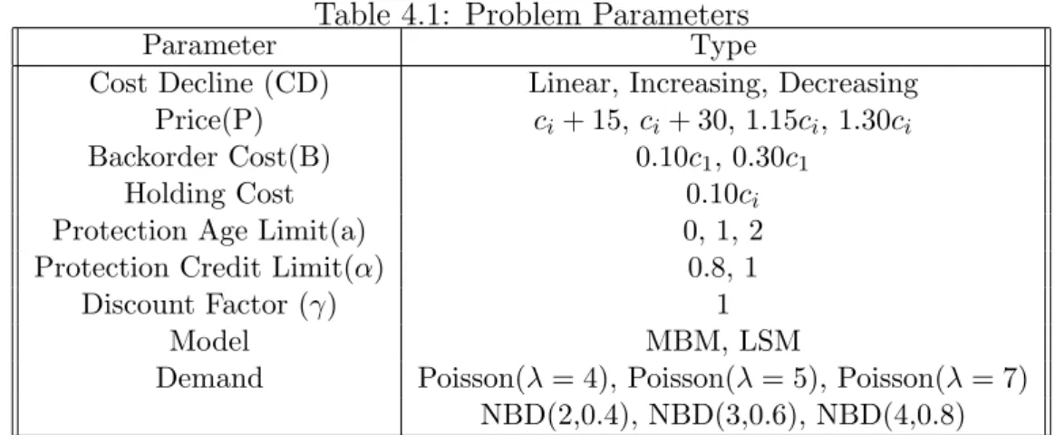
For both parts of the study, we are solving a 6-period problem with zero lead time and an ample supplier that offers the protection age limit to the retailer as one or two. We assume that the demand is stationary during the horizon. We explore the performance metrics’ responses under two different distributions that are Poisson and negative binomial (NBD). We study Poisson distribution under different means and NBD under different parameters that lead to the same mean but different variances. We assume that the discount factor is one throughout the horizon. Furthermore, we consider the problem parameters listed in Table 4.1 and the cost decline structures are listed in Table 4.2.
Table 4.1: Problem Parameters
Parameter Type
Cost Decline (CD) Linear, Increasing, Decreasing Price(P) ci+ 15, ci+ 30, 1.15ci, 1.30ci
Backorder Cost(B) 0.10c1, 0.30c1
Holding Cost 0.10ci
Protection Age Limit(a) 0, 1, 2 Protection Credit Limit(α) 0.8, 1
Discount Factor (γ) 1
Model MBM, LSM
Demand Poisson(λ = 4), Poisson(λ = 5), Poisson(λ = 7) NBD(2,0.4), NBD(3,0.6), NBD(4,0.8)
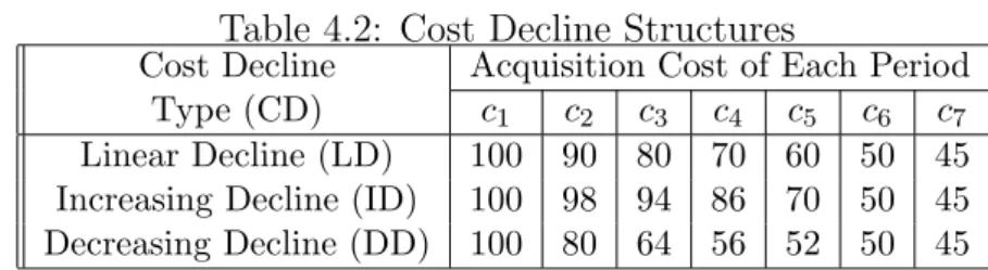
Table 4.2: Cost Decline Structures
Cost Decline Acquisition Cost of Each Period Type (CD) c1 c2 c3 c4 c5 c6 c7
Linear Decline (LD) 100 90 80 70 60 50 45 Increasing Decline (ID) 100 98 94 86 70 50 45 Decreasing Decline (DD) 100 80 64 56 52 50 45
The order-up-to levels and the expected profit of the retailer are derived by solving the dynamic programming formulation of the problem from the last period to the first one. At the end of the horizon, if the net inventory level at the retailer is greater than zero, the protection credit is calculated and paid to the retailer by the supplier in both MBM and LSM. If the retailer is operating with the MBM, the excess demand at the last period is assured to be satisfied by the retailer at the end of the horizon. If the retailer is operating with LSM, the excess demand at the last period is simply lost. The calculation of the expected profit of the retailer, expected cost for the protected items, expected revenue of the supplier, supplier’s profit, Type 1 and Type 2 service levels are done after determining the optimal order-up-to levels and feeding them into the simulation program that is coded in C. Each problem instance is run for 1500 replications. After completing the replications, the average of the related costs are determined and this process is repeated for all the problem instances we tabulated in Table 4.1. We choose the simulation in order to calculate the performance metrics since it is less complicated especially while computing the service levels. We double check the expected profit of the retailer with the result we obtained in the dynamic programming problem.
Price protection policy is costly from the supplier’s perspective since the sup-plier promises the reimbursement of the unsold inventory in the retailer’s stocks in case acquisition cost of the item declines. New component in the supplier’s costs is the protection cost. Cost component reflects the cost of increasing the availability of the product in the market (it is the cost of increasing flow rate of the newer products in the supply channel). The protection cost for the supplier obviously affects the supplier’s profit. It is intuitive that increasing protection
age limit or the credit, α, results higher protection costs and higher supplier’s revenue, however we cannot say much about the supplier’s profit as we do not consider ever cost component of the supplier here.
4.1
Modified Backorder Model
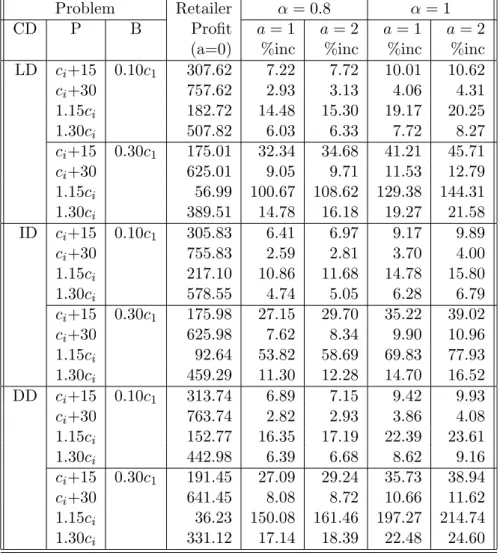
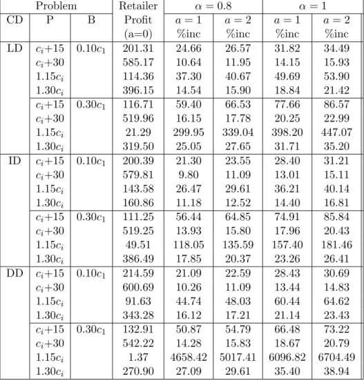
In all instances we observe that the profit of the retailer increases as the supplier increases the protection age limit or the credit. Table 4.3 shows the expected retailer profit when there is no price protection, and the percentage improve-ments on the expected retailer profit under different price protection terms when compared with the base case. We observe some instances where the retailer can increase his profit by 214.74% after the supplier introduces a protection policy to the chain. Therefore, the introduction of price protection policies make the retailer’s position better in comparison to the base case.
The minimum profit is attained by the retailer at all cost decline structures when the retailer is operating with higher backorder cost (0.30c1) and small profit
margin (1.15ci). Therefore, even a small increase in the retailer’s profit has a
significant effect as a percent increase. As a result, maximum percent increase in the retailer’s profit is achieved when the supplier introduces protection policies to the channel in these cases.
Table 4.3: Percent Increase in Retailer Profit Under Different Price Protection Policies (Poisson(λ = 5))
Problem Retailer α = 0.8 α = 1
CD P B Profit a = 1 a = 2 a = 1 a = 2
(a=0) %inc %inc %inc %inc LD ci+15 0.10c1 307.62 7.22 7.72 10.01 10.62 ci+30 757.62 2.93 3.13 4.06 4.31 1.15ci 182.72 14.48 15.30 19.17 20.25 1.30ci 507.82 6.03 6.33 7.72 8.27 ci+15 0.30c1 175.01 32.34 34.68 41.21 45.71 ci+30 625.01 9.05 9.71 11.53 12.79 1.15ci 56.99 100.67 108.62 129.38 144.31 1.30ci 389.51 14.78 16.18 19.27 21.58 ID ci+15 0.10c1 305.83 6.41 6.97 9.17 9.89 ci+30 755.83 2.59 2.81 3.70 4.00 1.15ci 217.10 10.86 11.68 14.78 15.80 1.30ci 578.55 4.74 5.05 6.28 6.79 ci+15 0.30c1 175.98 27.15 29.70 35.22 39.02 ci+30 625.98 7.62 8.34 9.90 10.96 1.15ci 92.64 53.82 58.69 69.83 77.93 1.30ci 459.29 11.30 12.28 14.70 16.52 DD ci+15 0.10c1 313.74 6.89 7.15 9.42 9.93 ci+30 763.74 2.82 2.93 3.86 4.08 1.15ci 152.77 16.35 17.19 22.39 23.61 1.30ci 442.98 6.39 6.68 8.62 9.16 ci+15 0.30c1 191.45 27.09 29.24 35.73 38.94 ci+30 641.45 8.08 8.72 10.66 11.62 1.15ci 36.23 150.08 161.46 197.27 214.74 1.30ci 331.12 17.14 18.39 22.48 24.60
Table 4.4 shows that the expected profit of the supplier when there is no price protection, expected protection cost and percentage improvements on the sup-plier’s profit under different price protection terms. The expected profit of the supplier is calculated by taking the difference between the expected revenue of the supplier and expected cost for the protected items.
Expected P rof it of the Supplier = Expected Revenue of the Supplier
We observe that the expected protection cost is non-decreasing in the protection age limit and credit. However, we cannot observe such a monotonicity for the supplier’s profit. Since it strictly depends on the problem parameters and order-up-to levels. Also, in most of the cases the supplier is hurt from protection policies. However, there are cases where win-win situation is observed. Therefore, if price protection policies are managed well, both of the players in the supply chain can be better off.
T able 4.4: Protection Cost and P ercen t Increase in Supplier’s Profit Under Differen t Price Protection P olicies (P oisson( λ = 5)) Problem Protection Supplier’s Protection Cost Supplier’s Profit % Increase CD P B Cost Profit α = 0. 8 α = 1 α = 0. 8 α = 1 a = 0 a = 0 a = 1 a = 2 a = 1 a = 2 a = 1 a = 2 a = 1 a = 2 LD ci +15 0.10 c1 0 2177.33 34.21 35.55 43.40 46.17 2.09 1.67 1.09 0.91 ci +30 0 2197.52 34.09 35.55 42.95 44.58 0.40 1.15 0.37 0.34 1.15 ci 0 2218.63 34.03 35.61 42.98 51.15 0.33 -0.36 -0.56 -0.61 1.30 ci 0 2194.57 34.54 36.67 48.53 63.32 0.72 0.21 0.37 1.58 ci +15 0.30 c1 0 2299.87 57.63 68.75 87.49 107.68 -1.69 -2.02 -3.04 -2.47 ci +30 0 2295.64 57.05 67.90 85.60 107.24 -1.21 -1.53 -1.82 -1.84 1.15 ci 0 2323.16 57.67 73.33 93.16 105.55 -2.85 -2.27 -.358 -2.30 1.30 ci 0 2311.00 57.09 79.44 92.64 113.65 -1.65 -1.60 -3.04 -1.79 ID ci +15 0.10 c1 0 2415.81 28.73 35.33 42.10 46.17 1.52 1.54 1.08 0.90 ci +30 0 2425.38 28.32 35.49 42.51 44.54 0.41 1.61 1.71 0.68 1.15 ci 0 2463.91 34.18 35.77 42.40 44.27 0.12 -0.55 -0.73 -0.89 1.30 ci 0 2440.08 34.17 37.09 54.94 66.52 0.41 -0.11 0.31 1.38 ci +15 0.30 c1 0 2523.92 57.21 62.55 72.96 103.67 -0.92 -1.54 -2.62 -1.72 ci +30 0 2503.95 56.45 61.41 74.12 106.17 0.20 -0.42 -2.05 -0.24 1.15 ci 0 2539.62 56.33 60.41 86.76 109.08 -1.65 -1.59 -2.61 -1.05 1.30 ci 0 2513.74 56.92 61.40 86.59 110.44 0.05 -0.58 -1.57 -0.19 DD ci +15 0.10 c1 0 1927.50 27.92 29.07 47.04 48.78 2.14 1.74 1.79 1.60 ci +30 0 1933.49 28.00 28.70 44.26 47.90 1.03 1.80 2.56 1.46 1.15 ci 0 1982.23 35.49 37.49 50.49 53.06 0.25 -0.45 -0.53 -0.85 1.30 ci 0 1969.68 37.00 38.49 60.22 62.31 0.16 -0.35 0.03 0.74 ci +15 0.30 c1 0 2047.97 65.56 71.05 84.30 100.75 -0.81 -1.57 -2.82 -2.22 ci +30 0 2033.11 65.46 70.59 84.81 97.46 0.15 -0.54 -2.30 -0.85 1.15 ci 0 2058.67 66.69 69.94 95.40 113.07 -1.63 -1.49 -2.81 -1.39 1.30 ci 0 2044.47 64.97 69.32 94.78 112.42 -0.19 -0.85 -2.12 -0.78