к & Ш ^ -ï. ¿ i ¿ w £ M« W ·(
тЬ
Tü£ tSáÓtíáÍl' Ё Ш Й Е Ü S M S S İklM ISI
ô f і * і ш т - і ш £ і е т т IM г Ш Ш і й Т Ш т ш ад-·2 2^· iS· - r ^ í í : Т Щ — « * ■*··'*»-^·— «ані к *» ^ ' ‘■m m' <»I' * f it ψ% r Г І ’ ' ч іа i î C i 'L y t h 'w М Д Е Т Ш й ? Ш № £ Ш Щ Ё Ш Ш Ш ^ М Ю М . //.. т:г Л Й 7 •А-^З / 5 Ä 2 ^ ^ п і Ц _ ’ί'.Λ л S' > ' s - «к лл, -1^ il Й. Й ír¡ Ti s У·. * " '*·^ ·*» f і' *І 4 V 'í *' ■■'■1 -'/ i í-· £j it и h i'. í - i j z) /INVENTORY CONTROL SYSTEM A CASE STUDY
A THESIS
SUBMITTED TO THE DEPARTMENT OF MANAGEMENT
AND THE GRADUATE SCHOOL OF BUSINESS ADMINISTRATION OF BILKENT UNIVERSITY
IN PARTIAL FULFILMENT OF THE REQUIREMENTS FOR THE DEGREE OF
MASTER OF BUSINESS ADMINISTRATION BY
NERİMAN KOCAOGLU FEBRUARY,1992
axci
Τ5
-/эбг ß т э т
-I certify that -I have read this thesis and in my opinion it is fully adequate, in scope and in quality, as a thesis for the degree of Master of Business Administration.
c __C ^ ^
Assist. Prof. Erdal Erel
I certify that I have read this thesis and in my opinion it is fully adequate, in scope and in quality, as a thesis for the degree of Master of Business Administration.
Assist. Prof. Dilek önkal
I certify that I have read this thesis and in my opinion it is fully adequate, in scope and in quality, as a thesis for the degree of Master of Business Administration.
r\
H J A u M j,.
Assist. Prof. Ümit Yüceer
ABSTRACT
INVENTORY CONTROL SYSTEM A CASE STUDY
Neriman Kocaoglu M.B.A.
Supervisor : Assist. Prof. Erdal Erel February 1992, 67 pages
There are two objectives of inventory control system. The first one is to maximize the level of the costumer service by having the right goods in sufficient quantities, in the right place, and at the right time. The other is to minimise the cost of providing the right level of customer service.
The inventory problem is to determine an ordering policy, determinig when to order and how much to order. In this study,an ordering policy is attempted to be determined for a small merchandise company. The A B C approach is one method to classify inventory items according to their importance. Different ordering policies could be used according to the result of A-B-C classification.
The required data are collected and processed in order to determine the ordering polic for each item.
Key words : Inventory control system, A-B-C classification, customer service level.
ÖZET
STOK KONTROL VAKA ANALİZİ Neriman Kocaoğlu Yüksek Lisans Tezi
Tez Yöneticisi : Y. Doç. Dr. Erdal Erel Şubat 1992, 67 sayfa
Stok kontrolün 2 amacı vardır. Bunlardan birisi müşteriye verilen hizmeti, doğru ürünü, doğru zamanda, doğru miktarda sunarak, en üst seviyeye çıkarmak, diğeri ise bu hizmeti verirken maliyeti en alt düzeyde tutmaktır.
Stok kontrolün en büyük problemi sipariş politikasını bel irleyerek, siparişin ne zaman ve ne kadar verileceğini belirlemektir. Bu çalışmada ufak bir ticari firma için, stok kontrol strategisi belirlenmeye çalışılmıştır. A-B-C klasifikasyonu ürünleri önemlerine göre ayıran bir metoddur. Bu metodla elde edilen sonuçlar doğrultusunda her ürün için bir stok kontrol mekanizması geliştirilebilir.
Her ürün için bir sipariş politikası belirleyebilmek için gerekli bilgiler toplanmış ve işlenmiştir.
Anahtar Kelimeler : Stok kontrol siştemi, A-B-C klaşifikas- yonu, müşteri serviş düzeyi.
ACKNOWLEDGEMENT
I would like to thank Assist. Prof. Erdal Erel for his supervision in the development of the thesis. I would also like to thank Assist. Prof. Dilek önkal and Assist. Prof, ümit Yüceer for their help. Finally I would like to thank to Faculty of Management of Bilkent University for providing me an invaluable MBA education.
TABLE OF CONTENTS
Subject Page
CHAPTER 1 - INTRODUCTION 1
1.1 - Problem Definition 1
1.2 - Important Factors For Decision Making 3
1.2.1 - Cost Factors 4
1.2.2 - Other Key Variables 5
1.3 - A-B-C Classification 5
1.4 - Thesis Outline 7
CHAPTER 2 - LITERATURE SURVEY 9 2.1 - An Order Quantity Decision System 9 2.2 - Decision System For Individual Item Under 11
Probabilistic Demand
2.2.1 - Three Key Questions To Be Answered by a 11 Control System Under Probabilistic Demand
2.2.2 - Continuous Versus Periodic Review 12 2.2.3 - Inventory Policies 13 2.2.4 - Choice Among Criteria For Establishing 14
Safety Stocks Of Individual Items
2.2.5 - Decision Rules For Continuous Review, 17 Order Quantity (s,Q) Model
2.2.5.2 - General Approach To Establishing 18 The Value Of s
2.2.5.3 - Decision Rule For A Given 19 Safety Factor (k)
2.2.5.4 - Decision Rule For A Specified Proba- 19 bility (PI) Of No Stockout Per
Replenishment Cycle
2.2.5.5 - Decision Rule For A Specified Average 19 Time Between Stockout Occasion
2.2.6 - Variability In The Replenishment Lead Time 20 Itself
2.3 - Discussion on A Items 20 2.4 - Discussion on For Managing Routine 22
( Class C ) Inventories
2.4.1 - Selecting The Reorder Point 22 2.4.2 - Stocking Versus Not Stocking An Item 23 CHAPTER 3 - INFORMATION ABOUT THE COMPANY 25 3.1 - General Information About The Company 25 3.2 - Company’s Inventory Policy 27
CHAPTER 4 - METHODOLOGY 28
4.1 - A-B-C Classification 28 4.2 - Stocking Versus Not Stocking An Item 28 4.3 - Choice Of The Inventory Policy 29 4.4 - How Much To Order And When To Order 29 4.5 - Choice Of Criteria For Establishing Safety 30
Stock Of Individual Items
4.5.2 - Choice Of Criteria For B Items 4.5.3 - Choice Of Criteria For C Items 4.6 - Analysis Of The Existing Policy 4.7 - Data Collection
4.8 - Data Processing CHAPTER 5 - RESULT
5.1 - Result Of The A-B-C Classification 5.2 - Stocking Versus Not Stocking An Item 5.3 - Goodness Of Fit Test
5.4 - How Much To Order, When To Order CHAPTER 6 - CONCLUSION REFERENCES APPENDIX VITA 31 32 32 36 42 42 42 45 46 49 52 53 67 31
LIST OF TABLES
Number Name Page
1 Suppliers And Lead Times 34 2 Unit Variable and Replenishment Costs 35
3 Demand In Units 37
4 E(L)’s And STD(L)’s 41
5 A-B-C Classification 43
6 Stocking Versus Not Stocking An Item 45
7 Goodness Of Fit Test 46
8 The Proposed Inventory Policy 47 9 The Existing Inventory Policy 48 10 Recommended And Existing Policy
Costs
50
Q-Replenishment order quantity, in units,
A-Fixed cost component associated with a replenishments, in do!lars.
v-Unit variable cost of the item, in $/unit. r-Carrying charge in $/$/unit time.
D-Demand rate, in units/unit time.
TRC(Q)-Total relevant cost per unit time, that is, the sum of those costs per unit time which can be influenced by the order quantity Q in $/unit time.
E(i)-Expected interval (or time) between demand transactions, in unit time.
E(t)-Expected size of a demand transaction, in units.
c(s)-System cost of having the item stocked, in $/unit time. k-Safety factor.
L-Replenishment lead time, in unit time. SS-Safety stock in units
E(L)-Expected demand over a replenishment lead time, in units.
STD(L)-Standard deviation of errors of forecast over a replenishment lead time, in units.
Pu(k)-Probabi1ity that a unit normal variable takes on a value k or larger.
1 - INTRODUCTION
Some two hundred years ago the management of inventories was, relatively, a simpler matter. Inventories were considered by merchants and producers as primarily a measure of wealth. Inventories are today viewed by most senior management as a large potential of risk and seldom as a measure of wealth. Most managers recognise the importance of balancing the advantages and disadvantages of carrying any level of inventory and try to manage inventory through the use of modern techniques.
1 . 1 - PROBLEM DEFINITION
Inventories are produced, used, or distributed by every organisation. They may be considered an accumulation of a commodity that will be used to satisfy some future demand for that commodity. Good inventory management is essential to the successful operation of most organisations. There are a number of reasons for this. First, inventories represent a major investment from the present perspectives of both individual firms and entire national economies. Enormous costs are incurred in the planning, scheduling, control, and carrying out of replenishment related activities. Another is
the impact that inventories have on the daily operations of an organisation. There has been tremendous progress in the technology of inventory control since 1957. But one basic fact remains: Inventory management is still a complex problem.
Inventories of an item should be justified by benefits accruing from functions served by inventories. Inventories are carried sometimes because of anticipated change in the cost of items, uncertainties in the future requirements and replenishment lead time. An important function of inventories is the improvement of customer service. In addition, inventories are related to economies of scale in production and procurement.
There are two main objectives in inventory control: Firstly, maximization of the level of customer service. Secondly, minimization of the high level customer service cost. Consequently, most of the inventory decisions are trade-offs
involving a compromise between the cost and customer service level.
Management need two supporting functions for inventory control. One is to establish a system of accounting for items in inventory, and the other is decision rules on how much to order and when to order. An effective management will need the following :
order. Inventory accounting system can be periodic or continuous.
b. A reliable demand forecast that includes an indication of possible forecast error.
c. Knowledge of lead-times and lead-time variability.
d. Accurate estimates of inventory holding costs, ordering costs, shortage costs, and system control costs.
e. A classification system for inventory items.
In this study, an inventory control system is applied to a company named AZTEK. This is a merchant company founded in May, 1990. The type of inventory that the firm holds is finished-goods or merchandise inventories. Currently, managers decide on the inventory without the use of any theoretical method.
The decision maker’s problem is to achieve a balance between overstocking as and understocking. Understocking results in missed deliveries, lost sales, dissatisfied customer and production bottlenecks, while overstocking unnecessarily ties up funds that might be more productive elsewhere. The two fundamental decisions that must be made relate to the timing and size of orders ( when to order and how much to order ).
1.2 - IMPORTANT FACTORS FOR DECISION MAKING
Through empirical studies and deductive mathematical modelling a number of factors have been identified that are
1.2.1 - Cost Factors
There are four basic costs that are associated with inventories; holding, replenishment, shortage and system control cost: [1]
important with respect inventory decisions.
Holding cost relates to physically holding items in storage. The cost of holding an item in inventory will depend naturally on its value, v, that is in conceptually equivalent to the price charged by outside suppliers plus other related variable costs such as transportation. Holding cost, for which the symbol r is assigned, also includes opportunity cost associated with having funds tied-up in inventory that could be used elsewhere. Holding cost also includes the cost of insurance, taxes, breakages and pi 1ferage at the storage site, warehouse rental and the cost of operating the warehouse such as labour. light etc. It is assumed that the system incurs damage costs. [2]
Replenishment cost is the costs associated with ordering and receiving the inventory. The cost of replenishment. A, is expressed as a fixed amount of money per order. The replenishment cost should include the cost of typing of orders, postage, telephone call inspecting goods upon arrival for quality and quantity.
Shortage cost result when demand exceeds the supply of inventory on hand. This cost has a different interpretation
depending on whether excess demand is backordered or lost. The cost can include the opportunity cost of not making a sale, loss of customer goodwill, lateness charges.[3]
System Control Cost include the costs of data acquisition, data storage and computation.
1.2.2 - Other Key Variables
Replenishment Lead Time L is the time that elapses from the moment at which an order is placed, until it is physically on the shelf for satisfying customer demands. The variability of demand over L is of importance.[13
Demand Pattern is another variable. Since inventory will be used to satisfy demand requirements, it is essential to have reliable estimates of the amount and timing of demand requi rements.
It is essential to know the extend to which demand and lead time might vary. The higher the variability, the greater the need for additional stock against shortages.[1]
1.3 - A-B-C CLASSIFICATION
An important aspect of inventory management concerns the fact that items kept in inventory are not of equal importance. Some items deserve more managerial attention than the others. Inventory management system can be improved upon by adopting
decision rules that do not treat all items equivalently. A priority can be assigned to each item in inventory according to its Dv value, assuming that item with higher annual dollar volume deserve more managerial attention. It is common to use three priority ratings or three classes of items: A (most important), B (moderately important) and C (least important). However the number of categories may vary from organisation to organisation depending on the circumstances and the degree to which a firm wishes to differentiate the amounts of effort allocated to various grouping of items. [4]
Other bases for an A-B-C classification are used. For example, some large volume consumer distribution centers plan the allocation of warehousing space on the basis of usage rate and cubic-feet square. [1]
Class A items should deserve close attention. The first 5 to 10515 of items which account for somewhere in the neighbourhood of 50% or more of the total annual dollar movement of all the inventories are usually classified as A items. Class B items should deserve a moderate but significant amount of attention. The largest number of items fall into this category. Usually 50% of items which account the most of the remaining 50% of annual dollar usage are classified as B items. When a computer facility is available as many item as possible can be controlled at a computer based system and class B items can be monitored as an A class item. [4]
Those items are remaining part that make up only a minor part of total dollar investment. For class C items decision systems must be kept as simple as possible. One objective of A-B-C classification is to identify this third group, which can potentially consume a large amount of data processing and record keeping time.
1.4 - THESIS OUTLINE
The second chapter is devoted to models that can assist in making two fundamental decisions on timing and size of orders
( when to order and how much to order ).
In Chapter 3, the case of AZTEK problem is described. The demand for the company’s items and its existing inventory policy are examined.
In Chapter 4, continuous review is justified as the most appropriate inventory accounting system. Accordingly (s,Q) model is chosen as the inventory policy. The choice of method for establishing safety stock depends on the class of item. The necessary data are collected and processed in the Data Collection and Data Processing sections for this purpose.
In chapter 5, the proposed inventory policy are developed for each item. In addition the existing inventory policy is analyzed.
compared with that of existing policy and the conclusions are delineated.
2 - LITERATURE SURVEY
Inventory control has been taught by academicians and used by practitioners for the last 75 years. Tremendous progress in the technology of inventory control system has been seen since 1957, especially after introduction of decision support systems. Traditional method is to keep inventory and establish a system of accounting for items in inventory and make decisions regarding how much to order and when to order.
2.1 - AN ORDER QUANTITY DECISION SYSTEM
Determining a replenishment quantity under rather stable conditions is of concern.There is relatively little or no uncertainty concerning the level of demand.
Basic EOQ Model
The basic EOQ model computes the order size that minimize the sum of the annual cost of holding inventory and ordering costs.
Assumptions :
Some of the assumptions may appear to be far away from reality but, the EOQ forms an important building block in the majority of decision systems .
a. The demand rate is constant and deterministic.
b. The order quantity need not be an integral number of units.
c. The unit variable cost does not depend on the replenishment quantity.
d. The item is treated entirely independent of other items. e. The replenishment lead time is zero.
f. No shortages are allowed.
g. The entire order quantity is delivered at the same time. [13
Some assumptions will be relaxed later.
Annual holding cost is computed by multiplying the average amount of inventory on hand by the cost of holding one unit for a year. The average inventory is simply one half of the order quantity, Q/2.
Annual holding cost = Qvr/2
Annual ordering cost is a function of the number of orders per year and the ordering cost per order.
Annual ordering cost = AD/Q + Dv
The second component is independent of Q and, hence, can have no effect on the determination of the best Q value. Therefore it will be ignored in further discussions.
TRC(Q)= Qvr/2 + DA/Q
TRC(Q) with Q.
Q* = SQR(2AD/vr) [5]
This is the economic order quantity. ( also known as the Wilson Lot size ) This is one of the earliest and most well known results of inventory theory.
The optimum policy calls for ordering Q* units every Q*/D time units. The optimal total annual cost TRC(Q*) can be expressed as follows:
TRC(EOQ) = SQR(2ADvr)
2.2 - DECISION SYSTEM FOR INDIVIDUAL ITEM UNDER PROBABILISTIC DEMAND
One of the assumptions in the determination of basic EOQ model is that the demand is deterministic. Deteministic demand assumption is inappropriate in many production and/or distribution situations. Shortage costs were not included in the analyses. A more realistic approach is the consideration of shortage costs in the model.[1]
2.2.1 - Three Key Questions To Be Answered by a Control System Under Probabilistic Demand
The main purpose of a inventory policy is to provide answers to the following three questions :
a. How often should the inventory status be monitored ? b. When should a replenishment order be placed ?
c. How large should the replenishment order be ?
Under the deterministic demand conditions the first question is trivial. Because when the inventory status at any one point in any time is known, to calculate it at all points in any time is allowed. Furthermore under deterministic demand conditions, the second question is answered by placing an order such that it arrives precisely when the inventory level hits some prescribed value (usually set at zero). EOQ is the answer of the third question.
Under probabilistic demand the answers are more difficult to obtain. Monitoring inventory status takes resources (labour, computer time, etc.). The answer to the second question rests upon a trade-off between the cost of ordering somewhat early hence carrying the extra stock, and the cost of providing inadequate customer service. EOQ can answer the third question. Probabilistic nature of demand affects the replenishment timing. [1]
2.2.2 - Continuous versus Periodic Review.
The answer to the question "How often should the inventory status be monitored?" specifies the review interval (R) which is the elapsed time between two consecutive moments at which we know the stock level. An extreme case is where there is continuous review. The stock status is monitored always and
R = 0. So the system can provide information on the status of item at all times. An obvious advantage of such system is the continuous monitoring of inventory withdrawals. One disadvantage of this approach is the added cost of record keeping. Many real world inventory systems are perpetual systems because of technological developments in computers and information processing.[6]
A periodic review system requires a physical count of items in inventory at periodic intervals, then necessary orders are placed. One advantage of this type of system is that orders for many items occur at the same time and there can be economies in processing and and shipping orders. An apparent disadvantage of periodic review is the lack of control between reviews. Another disadvantage is a need for protection against shortages between review periods by carrying extra stocks.
2.2.3 - Inventory Policies
There are several policies to consider. The four most common ones will be discussed. [1]
a. Order Point, Order Quantity (s,Q) Model : This model involves continuous review. A fixed quantity Q is ordered whenever the inventory position drops to the reorder point s, or lower.
b. Order Point, Order_Up_To_Level (s,S) Model : This model
again involves continuous review, and a replenishment is made whenever the inventory position drops to the reorder point s or lower. However in contrast to the (s,Q) model here a variable replenishment quantity is used, enough being ordering to raise the inventory position to the order up to level S.
c. Periodic Review, Order_Up_To_Level (R,s) Model : Every R units of time an order is placed to raise the inventory position to the level S.
d. (R,s,S) Model : Every R units of time an order is placed to raise the inventory position to the level S, if the level is below the order point s.
2.2.4 - Choice Among Criteria For Establishing Safety Stocks of Individual Items.
Under probabilistic demand there is a definite chance of not being able to satisfy some of the demand on a routine basis. Safety stock is proposed as an insurance against fluctuations in either demand or supply. It is often a necessary evil and should be kept as low as possible. [7]
If demand is unusually large emergency actions are required to avoid a stock_out occasion. On the other hand if demand is lower than anticipated, hence excess inventory is carried. Some methods to balance these two types of risks will be discussed next. [1]
a. Safety Stock Established Through The Use of a Common Factor.
Equal Time Supplies
This a simple, commonly used approach. The safety stocks of a broad group of items in an inventory are set equal to the same time supply; for example reorder any item when its inventory position minus the forecasted lead time demand drops to a 3-month supply or lower.
Equal Safety factors
It is convenient to define the safety factor (SS) as the product of factors as follows:
SS = kSTD(L) where k is called safety factor
STD(L) is the standard deviation of the errors of forecasts of total demand over a period of duration L.
b. Safety Stocks Based on the Shortage Costs Specified Fixed Cost(BI) per Stockout Occasion
The only cost associated with a stockout occasion is a fixed value B1, independent of the magnitude or duration of the stockout.
Specified Fractional Charge (B2) per Unit Short
A fraction B2 of unit value is charged per unit short of item i is B2v(i) where v(i) is the unit variable cost of the item.
Specified Fractional Charge (B3) per Unit Short per Unit Time A charge B3 per dollar short per unit time is used.
c. Safety Stock Based on Service Considerations.
Specified Probability (PI) of No Stockout per Replenishment Cycle
Equivalently, This is the fraction of cycles with no stockouts. A stockout defined as an event when the on-hand stock drops to the zero level. Using P1 across a group of
items is equivalent to using a common safety factor k. Specified Fraction (P2) of Demand To Be Satisfied Routinely from the Shelf (that is, Not Lost or Backordered)
A form of service measure with considerable appeal to practitioners is the specification of a certain fraction of customer demand that will be met routinely.
Specified Ready Rate (P3)
The ready rate is the fraction of time during which the net stock is positive.
Specified Average Time Between Stockout (TBS) Occasions
Equivalently, one could use the reciprocal of TBS, which represents the desired average number of stockout occasions per year.
Unfortunately there are no hard and fast rules for selecting the appropriate approach and/or measure of service which to
use depends on the environment of the particular company under consideration.
2.2.5 - Decision Rules For Continuous-Review, Order-Quantity (s,Q) Model
The choice of criterion for safety stocks is a strategic decision. Senior management must be involved directly. Once a criterion is selected, there is then the tactical issue of the selection of a value of the associated policy variable.
(For example, the numerical value of P2 for that particular service measure.) [1]
2.2.5.1 Common Assumptions and Notations
There are a number of assumptions on the methods of estimating costing shortage or measuring service. These are: a. Although demand is probabilistic, the average demand changes very little with time.
b. A replenishment order of size Q is placed when the inventory level is exactly at the order point s.
c. If two or more replenishment orders for the same item are simultaneously outstanding, then they must be received in the same order in which they were placed.
d. Unit shortage costs are so high that a practical operating procedure will always result in the average level of backorders being negligible small when compared with the average level of the on hand stock.
e. Forecast errors have a normal distribution with no bias and a known standard deviation STD(L) for forecast over a
lead time L.
f. Where a value of Q is needed, it is assumed to have been predetermined.
g. The cost of control system does not depend on the specific value of s selected.
Common notations include:
D = demand rate in units/year
Gu(k) = a special function of the unit normal variable, k = safety factor
L = replenishment lead time, in years
Pu(k) = probability that a unit normal variable takes on a value of k or larger
Q = prespecified order quantity, in units SS = safety stocks in units
V = unit variable cost, in $/unit
E(L) = forecast (or expected) demand over a replenishment lead time, in units
STD(L) = standard deviation of errors of forecasts over a replenishment lead time, in units [1]
2.2.5.2 - General Approach To Establishing The Value Of s Reorder Point, s = x(L) + ( safety stock )
and
where k is known as the safety factor. Determination of a k value leads directly to a value of s.
2.2.5.3 - Decision Rule for a Given Safety Factor (k) Once k value is specified;
The Rule
Step 1 Safety stock, SS = kSTD(L)
Step 2 Reorder point, s = E(L) + SS, increased to the next integer.
2.2.5.4 - Decision Rule for a Specified Probability (PI) of No Stockout Per Replenishment Cycle
Suppose management has specified that the probability of no stockout in a cycle should be no lower than P1.
The Rule
Step 1 Select The safety factor k to satisfy Pu(k) = 1 - PI
Step 2 Reorder point, s = E(L) + kSTD(L), increased to the next higher integer.
2.2.5.5 - Decision Rule for a Specified Average Time Between Stockout (TBS) Occasion
The Rule Step 1 is
If Q/D(TBS) > 1 Yes, then go to Step 2
Else Select a safety factor k to satisfying Pu(k) = Q/D(TBS)
if the resulting k is lower than the minimum allowable value specified by management then go to step 2. Otherwise, move to Step 3.
Step 2 Set k at its lowest permitted value.
Step 3 Reorder point, s = E(L) + kSTD(L), increased to the next higher integer.
2.2.6 - Variability in the Replenishment Lead_Time Itself
If L is not known with certainty it is apparent that increased safety stock is required as protection against this additional uncertainty.
If L and D are assumed to be independent random variables, then it can be shown that
and
E(x) = E(L)E(D)
STD(x) = SQR( E(L)VAR(D) + (E(D))2VAR(D) [4]
2.3 - DISCUSSION ON A ITEMS
importance. The total cost of replenishment, holding stock and shortage associated with such an item is high enough to justify a more sophisticated control system.
The factor Dv is important in deciding on whether or not to place an item in the A category. However the type of policy to use within the A category should definitely depends upon the magnitudes of the individual components, D and v. A high Dv value resulting from a low D and a high v value implies a different policy from a high D and a low v value. [1]
Section 2.2 discusses the use of the normal distribution to represent the distribution of forecast errors over a lead time. The potential benefits of using a more accurate representation for A items is higher. It is suggested still using the normal distribution if the demand is normally distributed. Typical management behaviour is to cope with potential or actual shortages of A items. If distribution is not normal, a discrete distribution such as Poisson is likely more appropriate. [1]
The Poisson distribution has a single parameter, namely, the average demand (in this case E(L)). Once E(L) is specified, a value of the standard deviation of forecast errors, STD(L), follows from the Poisson relation
STD(L) = SQR(E(D)
Therefore, the Poisson distribution is appropriate to use when the actually observed standard deviation of demand during a replenishment lead time, STD(L), is quite close to
the squared of expected demand, E(L).
The distribution of demand during a replenishment lead time could be tested by goodness-of-fit test. This is a statistical test checking the validity of a hypothesized probability distribution for a population. [8]
2.4 - DISCUSSION ON MANAGING ROUTINE ( CLASS C ) INVENTORIES
The primary factor which indicates that an item should be placed in C category is low dollar usage ( Dv value ). As the C type item should receive only loose control. Using simple procedures keeps the control costs quite low and labour and paperwork per item will be at a minimum. In selecting the reorder quantity basic EOQ should be used. [1]
2.4.1 - Selecting the Reorder Point
One may choose any of the criteria discussed in section 2.2 for selecting a safety factor. Selecting a safety factor to provide a specified expected time between stockout (TBS) occasions is accurate. This approach appeals to the management for most C items. Thinking in terms of an average time between stockouts is rather straightforward than dealing with probabilities or fractions. [1]
factor k to satisfy Pu(k) = ( Q/D(TBS)) where
Pu(k) = Prob { Unit normal variable takes on a value of k or larger }
Then the reorder point is s = X(L) + kSTD(L)
2.4.2 - Stocking Versus Not Stocking an Item
Satisfion of customer demand for an item the following question needs an answer : Should a special order be placed to satisfy each individual customer demand transaction or keep the item in stock ?
A Simple Decision Rule Assumptions
a. The unit variable cost is the same under stocking and nonstocking
b. The fixed setup cost is the same under stocking and nonstocking.
c. In deriving the decision rule to decide on whether to stock the item or not, the order quantity is allowed to be a noninteger (of course, if the item was actually stocked and demands were in integer units, an integer value for the order quantity).
d. The replenishment lead time is negligible; there is no backordering cost.
The Decision Rule
Do not stock the item if either of the following two conditions holds (otherwise stock the item):
c(s) > A/E(i) or
E(t)vr > (E(i)/2A)(A/E(i)-c(s)) where
c(s) = system cost, in dollars per unit time, of having the item stocked
A = fixed setup cost, in dollars, associated with a replenishment
E(i) = expected (or average) interval (or . time) between demand transaction
E(t) = expected (or average) size of a demand transaction in units
V = unit variable cost of the item, in $/unit r = holding charge, in $/$/unit time [1]
Characteristics of the inventory control system are discussed. Now it is time to choose the models that can be applied in assisting on fundamental decisions relate to the timing and size of orders.
Next chapter presents the methodology with which the decisions are made.
3 - INFORMATION ABOUT THE COMPANY
3.1 - GENERAL INFORMATION ABOUT THE COMPANY
AZTEK is a merchandising company that was founded by two partners in May 1990. The company sells a variety of household appliances, in which sell expansion has been substantial. The company’s annual sales volume is approximately TL 3 billion.
The head office of the company is located in downtown and it has a store almost two kilometres away from the head office. The employee profile is made up of three workers. One of them is does marketing and the others do deliveries.
AZTEK sells the majority of its items through retailing stores and the minority through distributors. Buyers consider price to be the most important factor in determining from whom they will buy the appliances. They consider delivery service the second important factor.
Seasonality and changes in prices are two most important risks. The company owners have just added another unwelcome item to their worry list : high competition. The number of competitors, which is six now, varies depending on the economical conditions, but the competition is quite high.
Success requires competing on terms other than price, such as speed of delivery.
Therefore an efficient and effective inventory management becomes necessary. Managers realise that a number of changes are needed in many parts of company’s inventory control system. The price is determined by adding a fixed percentage to the buying price. This percentage varies from item to item according to the competitors attitudes. Another problem that managers are faced is the problem of fluctuations in sales volume. As long as fluctuations exists, the company has a problem in demand forecasting.
The company has sufficient space. There is no upper limit on the number of orders to place and no upper limit on the maximum dollar investment in inventory.
In purchasing, vendor often offer price discounts if the purchase quantity is large. Quantity discount is not applicable to AZTEK.
Backordering is well accepted by customers. The inventory could become out of stock due to two reasons. One is the access demand, the other one is the limited production of the i terns.
The company purchases sixteen types of household appliances from five suppliers. The lead times are constant for each supplier. The items their supplier and lead-time is given
in Table 1
3.2 - COMPANY’S INVENTORY POLICY
The management of the company makes all the decisions merely by intuition and experience. No classification method is used for the arrangement of the items according to their importance. The existing inventory policy of the company have some rules explained below.
Usually an order is placed when the inventory level drops down to zero level. In other words, an extra stock is carrying but there is not a strict control to handle the stockouts during a lead time. The management tries to forecast the demand while determining the order quantity.
Characteristics of the problem are defined, so that inventory policy of the company can in turn be chosen. Next chapter presents the methodology with which the problem is approached.
4 - METHODOLOGY
4.1 - A-B-C CLASSIFICATION
As an inventory management system can be significantly improved by simply adopting decision rules that do not treat all items equivalently, A-B-C type of classification is used. As AZTEK is a retailer company, the classification is based on annual TL volume (Dv).
4.2 - STOCKING VERSUS NOT STOCKING AN ITEM
Appropriate answer to the question of whether or not an item is stocked can yield substantial savings. The procedure of the decision rule is applied for C class items.
The Decision Rule
Do not stock the item if either of the following two conditions holds (otherwise stock the item)
c(s) > A/E(i) (1) or
E(t)vr > SQ(E(i)/2A)(A/E(i)-c(s)) (2)
All of the variables can be estimated easily except c(s) which is the system cost. Therefore Eq. 2 is used in determining whether or to stock the item or not. It is assumed that c(s) = 0. Then Eq. 2 reduces to :
Do not stock the item if following condition holds (otherwise do stock)
E(t)vr > A/2E(i)
4.3 - CHOICE OF THE INVENTORY POLICY
Continuous review is chosen as the inventory accounting system. The company already owns a computer, and the added cost of record keeping will be low. The number of items is not large, which makes continuous monitoring of inventory possi ble.
A further step is use of (s,Q) or (s,S) model as the inventory policy (s,Q) is a simple model to understand, while (s,S) model need a computational effort to find the best (s,S). The risk of making error is high. On the other hand, (s,S) model can be shown to have total costs of replenishment, holding inventory and shortages no larger than those of the best (s,Q) model. As a result, (s,Q) model is chosen as the inventory policy due to its simplicity.
4.4 - HOW MUCH TO ORDER AND WHEN TO ORDER
The question of how much to order is answered by using the economic-order-quantity, EOQ.
EOQ = SQR(2AD/vr)
The question of when to order is answered by finding the reorder point, s.
Reorder point, s = E(L) + kSTD(L) The total cost of holding inventory is
TRC(Q) = Qvr/2 + AD/Q
when a reorder point is determined TRC(Q) becomes, TRC(Q) = (Q/2 + s)/2 + AD/Q
If an item is not stocked, the amount to order will be equal to the demand itself. Total cost is than :
TRC(Q) = AN
where N is equal to the number of demand transaction in a year.
4.5 - CHOICE OF CRITERIA FOR ESTABLISHING SAFETY STOCK OF INDIVIDUAL ITEMS
There are some methods to balance the risk of running out of stock and carrying excess inventory. The choice of method for establishing safety stocks depends on the class of the item.
4.5.1 - Choice of Criteria for A items
The use of costing of shortages is recommended for A items. [1] That will require estimating B1, B2 or B3. It is very difficult to estimate the cost of shortages especially as in the case of AZTEK, there is no data available. An alternative approach could be the use of a desired level of customer service. Therefore instead of making errors in calculations.
it is better to specify a desired level of consumer service. Additionally in the case of a stockout, the percentage of
lost sales is not high. As a result the estimate of specified probability (PI) of no stockout per replenishment cycle is chosen for A items as a service measure.
4.5.2 - Choice of Criteria for B Items
In establishing safety stocks for B items, any criterion in section 2.2.4 for selecting the safety factor may be chosen. As the items are not numerous, the method that is used for A
items may be used for B items as well. An estimate of specified probability (PI) of no stockout per replenishment cycle should be specified.
4.5.3 - Choice of Criteria for C Items
C items represent a very small fraction of the total TL investment in the inventory, these items are considered relatively unimportant. Establishing a safety stock for these is rather straightforward if an average time between stockouts is considered. Large values of TBS are not reasonable when one recognise the added expense of holding a high safety stock.
The distribution of demand during a replenishment lead time for A items is tested by goodness-of-fit test. For the case of B items the normal distribution provides a good
representation of the distribution of forecast error over a lead time.
P1 is set to 0.20 judgmental!y, therefore k is equal to 0.84. Additionally TBS for C items is given as 1 month.
4.6 - ANALYSIS OF THE EXISTING POLICY
Annual holding cost is computed by the average amount of inventory on hand by the cost of holding one unit for a year.
Holding Cost = E(I)vr
E(I) is the average inventory
E(I) = (Amount of order * Days) / Days where
Days = number of days between orders. N = number of orders
Annual ordering cost is a function of the number of orders. Ordering Cost = AN
where
N = number of orders.
4.7 - DATA COLLECTION
The required data have to be collected for computing the costs and other key variables of inventory system. Consulting with management and past data are obtained for this purpose.
There are sixteen different items in the inventory, each having different characteristics, shown in Table 1. The number of items is small, different method is applied to each of item. Because the methods that are used here could be applied to any other company that has large number of item. Therefore, for all of those items the data are obtained except HLJNSB. A contract is signed between AZTEK and suppliers of HLJNSB in which the price and the amount are determined on a yearly basis. This item is then excluded from the inventory control study.
Replenishment lead time, L, depends on the supplier rather than the item itself. The well known suppliers are utusan, Intratek, Bimex, ugur Makina and Tamsel. Lead time data are obtained from the management. It is constant for each item. Unfortunately there is not a database to measure the variability of lead time. The suppliers and lead times for each item are shown in Table 1.
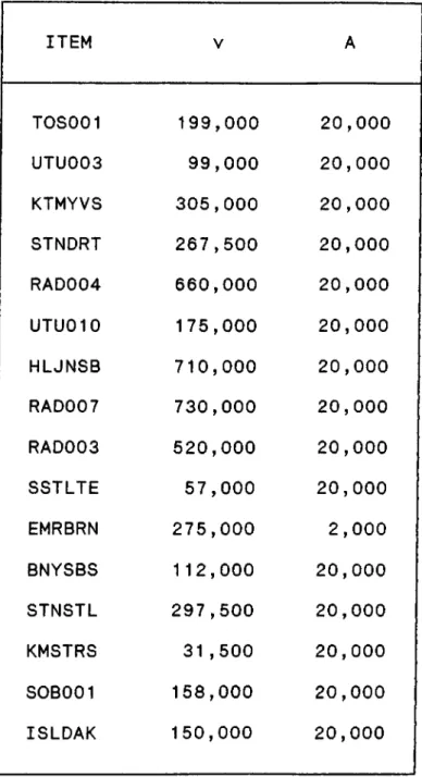
Setup cost. A, the unit value, v, data are also obtained from the management. Setup cost includes only the telephone call. A and V of each item is shown in Table 2.
The company owns storage space for inventory. This idle space is not suitable for generating revenue. There are no costs of insurances and damages. Therefore, inventory holding cost is just the opportunity cost of tying money in inventory. It is taken as the annual interest rate. The interest rate, r, is
TABLE 1. SUPPLERS AND LEAD TIMES
ITEM SUPPLIER LEAD TIME (in days) TOS001 Utusan 3 UTU003 Otusan 3 KTMYVS utusan 3 STNDRT Ugur Makina 4 RAD004 Otusan 3 UTU010 utusan 3 HLJNSB Intratek 4 RAD007 utusan 3 RAD003 utusan 3 SSTLTE utusan 3 EMRBRN Tamsel 3 BNYSBS utusan 3 STNSTL utOsan 3 KMSTRS Bimex 4 SOB001 Otusan 3 ISLDAK Intratek 4
TABLE 2. UNIT VARIABLE AND REPLENISHMENT COSTS ITEM V A TOS001 199,000 20,000 UTU003 99,000 20,000 KTMYVS 305,000 20,000 STNDRT 267,500 20,000 RAD004 660,000 20,000 UTU010 175,000 20,000 HLJNSB 710,000 20,000 RAD007 730,000 20,000 RAD003 520,000 20,000 SSTLTE 57,000 20,000 EMRBRN 275,000 2,000 BNYSBS 112,000 20,000 STNSTL 297,500 20,000 KMSTRS 31,500 20,000 SOB001 158,000 20,000 ISLDAK 150,000 20,000 35
obtained also from the management.
Sales transaction for each item are examined carefully. Last one year’s data (from December 1990 to November 1991) are collected as the sales transaction. The demand is seasonal for KTMYVS, RAD004, RAD007, RAD003, STNSTL, KMSTRS, SOB001 and ISLDAK.
Management expect that the annual demand D will be very much like the last year’s annual demand. A naive approach is used as the forecasting method.[4]
In order to analyse the existing policy ordering data are also collected,
4.8 - DATA PROCESSING
Data are processed to obtain inputs for the inventory control.
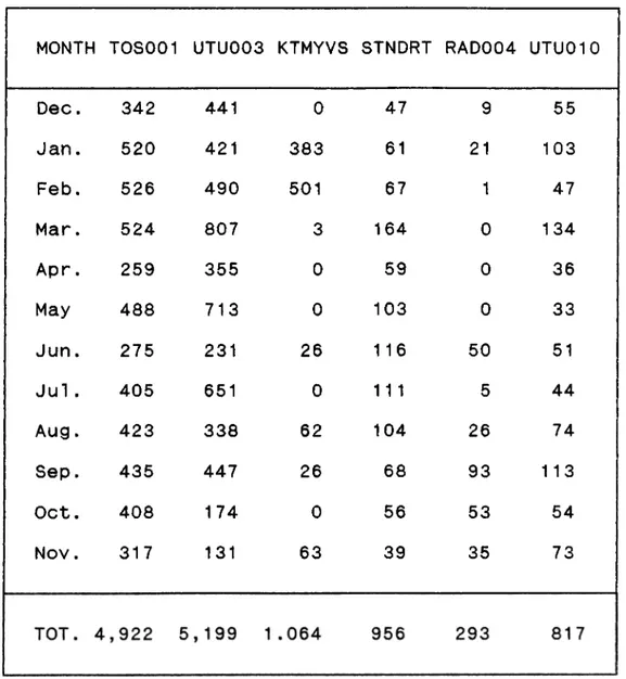
First Annual demand D is found for each item, by taking the sum of all monthly sales transactions of the last year. Monthly sales are given in Table 3. Annual TL value, Dv, is calculated for each item. Then percentage of each item and its percentage of TL usage are determined.
The decision rule on stocking versus not stocking an item requires the values of E(i) and E(t). E(i) is the expected interval between demand transactions, and found by counting the daily sales which are zero. E(t) is the expected size of
TABLE 3. DEMAND IN UNITS
MONTH TOS001 UTU003 KTMYVS STNDRT RAD004 UTU010 Dec. Jan. Feb. Mar. Apr. May Jun. Ju1 . Aug. Sep. Oct. Nov. 342 520 526 524 259 488 275 405 423 435 408 317 441 421 490 807 355 713 231 651 338 447 174 131 0 383 501 3 0 0 26 0 62 26 0 63 47 61 67 164 59 103 116 1 11 104 68 56 39 9
21
1
0 0 0 50 5 26 93 53 35 55 103 47 134 36 33 51 44 74 113 54 73 37TABLE 3 (CONTINUED)
MONTH HLJNSB RAD007 RAD003 SSTLTE EMRBRN BNYSBS
Dec. J a n . Feb. M a r . A p r . May J u n . Ju1 . A u g . Sep. Oct. Nov. 39 3
1
0 0 0 0 0 71 24 61 71
5 0 0 0 0 41 6 18 4021
27 0 0 0 0 0 23 48 5 22 26 54 32 40 233 67 231 90 283 33 51 81 43 98 6121
1
13 14 3 12 35 010
9 0 3 01
9 30 2 0 21
011
1
49 82 TOT. 206 159 210 1,311 121 817TABLE 3 (CONTINUED)
MONTH STNSTL KMSTRS SOB001 ISLDAK
Dec. 0 202 0 0 Jan. 0 227 0 0 Feb. 0 39 0 0 Mar. 0 49 0 0 Apr. 9 0 0 0 May. 17 0 0 0 Jun. 13 0 2 28 Jul . 15 0 3 6 Aug. 7 0 15 12 Sep. 0 0 1 19 Oct. 2 36 18 0 Nov. 4 16 42 2 TOT. 67 569 81 67 39
a demand transaction in units and is found by taking the average of sales which are not zero.
r is the holding charge is 8% per month. Daily or annual holding charge is found by using Eq. 3.
r = (1+i)"period - 1 (3)
For testing, whether the distribution of demand during lead time is normal or not for A items, Goodness-of-fit test is used. Lead time demand transactions are obtained by adding the daily demands during a lead time. For instance, when the lead time is equal to 3 days, the sum of daily demand is taken for each of 3 days. Table 4 provides expected demand during a lead time, E(L), and its standard deviation of demand during a lead time, STD(L). Upper and lower tails of the normal distribution is found by the equation E(L) -(+) 2STD(L) and a number of categories, k, is calculated by taking the sqareroot of the number of lead time demand transaction.
Expected frequency for each category is found by multiplying the probability of being in a category and the number of lead time demand transaction. Observed frequency, 0(j), for each each category is found by counting the number of transaction which is in this category.
TABLE 4. E(L)’s and STD(L)’s
ITEM E(L) STD(L) PERIOD (in month) TOS001 51.64 40.04 A11 UTU003 54.73 59.53 All
KTMYVS 52.06 41.02 Jan. to Feb. KTMYVS 4.02 7.39 June to Nov. STNDRT 13.47 11.46 All
RAD004 4.87 6.59 June to Dec. UTU010 8.60 11.76 A11
RAD007 3.39 4.23 June to Nov. RAD003 4.20 5.30 May to Nov. STLLTE 13.80 25.94 All
KMSTRS 16.26 22.21 Oct. to Mar. SOB001 2.38 4.48 Aug. to Nov. ISLDAK 2.71 3.75 June to Sep.
The analysis of the existing policy will need number of orders, N, and number of days between orders.
5 - RESULT
5.1 - RESULT OF THE A-B-C CLASSIFICATION
The percentage of item that accounts approximately 50% of annual TL usage is 12.5%.Intuitively, TOS001 and UTU003 have a relatively high annual TL value. It makes sense to classify them as A items.
Availability of computer facility allows to classify as many items as possible as B items. KTMYVS, STNDRT, RAD004, UTU010 HLJNSB, RAD007 and RAD003 appear to have moderate annual TL values and should be B items.
The remaining items, STLLTE, EMRBRN, BNYSBS, STNSTL, KMSTRS, SOB001 and ISLDAK should be C items based on their relatively low TL usage. The results are shown in Table 5 and Figure 1.
5.2 - STOCKING VERSUS NOT STOCKING AN ITEM
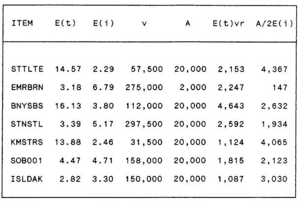
There are three items, EMRBRN, BNYSBS and STNSTL, that E(t)vr is greater than A/2E(i). The results are shown in Table 6. Therefore for those three items a special purchase will be made from the supplier to satisfy each individual customer demand. The remaining items, SSTLTE, KMSTRS, SOB001 and ISLDAK, will be stocked.
TABLE 5. A-B-C CLASSIFICATION
INV. ANNUAL UNIT ANNUAL CUM %
CODE DEMAND COST TL VOL. ITEM SUM OF TL CUM % TL
TOSCO1 UTU003 KTMYVS STNDRT RAD004 HLJNSB UTU010 RAD007 RAD003 SSTLTE EMRBRN BNYSBS STNSTL KMSTRS SOB001 ISLDAK 4922 5199 1064 956 293 817 199 159
210
1311121
205 67 569 81 67 199000 99000 305000 267500 660000 175000 710000 730000 520000 57500 275000112000
297500 31500 158000 150000 979478000 514701000 324520000 255730000 193880000 142975000 141290000 116070000 109200000 75382500 33275000 22960000 19932500 17923500 12798000 10050000 6.3 12.5 18.8 25.0 31.3 37.5 43.8 50.0 56.3 62.5 68.8 75.0 81.3 87.5 93.8100.0
979478000 1494179000 1818699000 2074429000 2267809000 2410784000 2552074000 2668144000 2777344000 2852726500 2886001500 2908961500 2928894000 2946817500 2959615500 2969665500 33.0 50.3 61.2 69.9 76.4 81.2 85.9 89.8 93.5 96.1 97.2 98.0 98.6 99.2 99.7100.0
43si
TABLE 6. STOCKING VERSUS NOT STOCKING AN ITEM
ITEM E(t) E(i ) V A E(t)vr A/2E(i)
STTLTE 14.57 2.29 57,500 20,000 2,153 4,367 EMRBRN 3.18 6.79 275,000 2,000 2,247 147 BNYSBS 16.13 3.80 112,000 20,000 4,643 2,632 STNSTL 3.39 5.17 297,500 20,000 2,592 1,934 KMSTRS 13.88 2.46 31,500 20,000 1,124 4,065 SOB001 4.47 4.71 158,000 20,000 1,815 2,123 ISLDAK 2.82 3.30 150,000 20,000 1 ,087 3,030
5.3 - GOODNESS OF FIT TEST
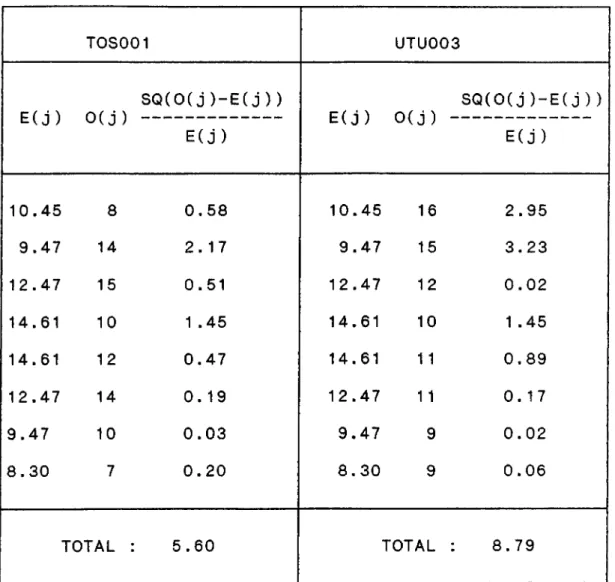
Goodness-of-fit test is applied to A items. The Chi_square distribution has k-1 degrees of freedom. Therefore the degree of freedom is 7 for both TOS001 and UTU003 . The level of significance, p, is taken as 0.10. As the p value is less than 0.1 for both item the hypothesis of the normal distribution is accepted. Calculations are given in Table 7.
TABLE GOODNESS OF FIT TEST
TOSCO1 UTU003
E(j) 0(j) SQ(0(j)-E(j)) E(j) n i ^ SQ(0(j)-E(j))
E(j) E(j) 10.45 8 0.58 10.45 16 2.95 9.47 14 2.17 9.47 15 3.23 12.47 15 0.51 12.47 12 0.02 14.61 10 1 .45 14.61 10 1 .45 14.61 12 0.47 14.61 11 0.89 12.47 14 0.19 12.47 1 1 0.17 9.47 10 0.03 9.47 9 0.02 8.30 7 0.20 8.30 9 0.06 TOTAL : 5.60 TOTAL : 8.79
5.4 - HOW MUCH TO ORDER, WHEN TO ORDER
The answers to these questions will be determined next for each item. The proposed inventory policy is presented in Table 8.
TABLE 8. THE PROPOSED INVENTORY POLICY
ITEM EOQ s TRC(Q) PERIOD (in month)
TOSCO1 26 85 18,002,714 A11 UTU003 37 105 10,307,880 All
KTMYVS 26 87 3,116,950 Jan. to Feb. KTMYVS 5 10 1,997,575 June to Nov. STNDRT 10 23 8,011,000 A11
RAD004 5 10 5,936,500 June to Dec. UTU010 1 1 18 5,608,455 All
RAD007 4 7 3,379,200 June to Nov. RAD003 5 8 3,239,300 May to Nov. STLLTE 24 34 3,889,300 All
EMRBRN - - 98,000 All
BNYSBS - - 580,000 All
STNSTL - - 420,000 Apr. to Nov.
KMSTRS 35 24 780,475 Oct. to Mar. SOB001 7 6 635,960 Aug. to Nov. ISLDAK 7 3 632,000 June to Sep.
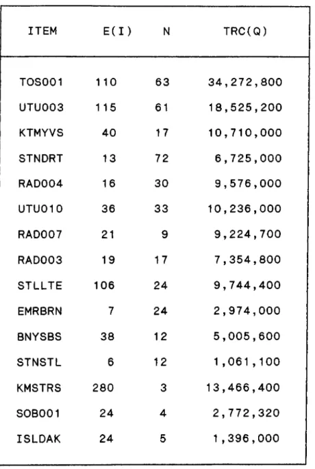
The existing inventory policy is given in Table 9,
TABLE 9. THE EXISTING INVENTORY POLICY ITEM E(I) N TRC(Q) TOSCO1 110 63 34,272,800 UTU003 115 61 18,525,200 KTMYVS 40 17 10,710,000 STNDRT 13 72 6,725,000 RAD004 16 30 9,576,000 UTU010 36 33 10,236,000 RAD007 21 9 9,224,700 RAD003 19 17 7,354,800 STLLTE 106 24 9,744,400 EMRBRN 7 24 2,974,000 BNYSBS 38 12 5,005,600 STNSTL 6 12 1,061,100 KMSTRS 280 3 13,466,400 SOB001 24 4 2,772,320 ISLDAK 24 5 1,396,000
Calculations of the TRC(Q) for the both policies are provided Conclusion are discussed in the next chapter.
6 - CONCLUSION
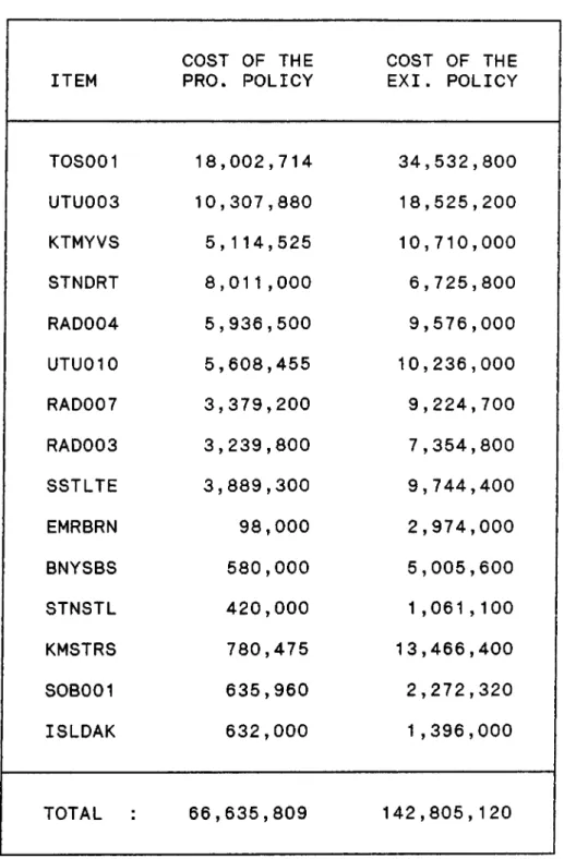
The total annual cost associated with holding and ordering inventory for the proposed policy is TL 66,635,809 and for the existing policy it is TL 142,805,120 which is given in Table 10. There is a savings of TL 76,169,311 (53%). The main difference between the company’s existing policy and proposed policy for A and B class items is the inventory level. In the proposed policy the inventory level is lower than the existing policy, except for the STNDRT and the savings is TL 24,747,406(47«) for A items and TL 22,537,820
(42«) for B items.
There are two main differences between existing and proposed policy for C class items.
1. The company does not care whether a C item should be stocked or not. It stocks all the C items.
2. The inventory levels for to be stocked C are lower in the proposed policy.
There is a big savings TL 28,884,085 (80«). It is highly recommended that the company should adapt the new proposed inventory policy especially for C items.
The proposed policy is obtained by some analytical techniques
TABLE 10. PROPOSED AND EXISTING POLICY COSTS
ITEM COST OF THE PRO. POLICY COST OF THE EXI. POLICY
TOS001 18,002,714 34,532,800 UTU003 10,307,880 18,525,200 KTMYVS 5,114,525 10,710,000 STNDRT 8,011,000 6,725,800 RAD004 5,936,500 9,576,000 UTU010 5,608,455 10,236,000 RAD007 3,379,200 9,224,700 RAD003 3,239,800 7,354,800 SSTLTE 3,889,300 9,744,400 EMRBRN 98,000 2,974,000 BNYSBS 580,000 5,005,600 STNSTL 420,000 1,061,100 KMSTRS 780,475 13,466,400 SOB001 635,960 2,272,320 ISLDAK 632,000 1,396,000 TOTAL : 66,635,809 142,805,120
and provides savings of 53%. If the company uses an analytical method, it will gain a risk-free TL 76,169,311. Changing times would require changes in costs and in portfolio of items. Without the use of analytical methods, the efficient and effective management of inventory will not be materi ali zed.
Two types of risks overstocking and understocking are balanced by using theoritical methods. Classification of items and usage of an inventory control system maximized the customer service level and minimized the costs. At the next step more data can be collected by the company which unables the analyser to get the shortage and system costs. A more sensitive analysis can be made by adding those costs to the total cost formula.
There are several other companies merchandising household appliances. The proposed policy can be adopted to those companies as well.
In conclusion, AZTEK and the sector can achieve large savings. This analytical inventory approach can be adapted to the changing conditions to help management and to search better and effective inventory policies
REFERENCES
1. Peterson R. and Silver EA (1979) Decision Systems For Inventory Management and Production Planning John Wiley & Sons, Inc., NY.
2. Chyr F., Lin T. and Chin_Fu (1989) An extension of the EOQ Production Model Based on Damage Costs.
3. Nahmias S. (1989) Production and Operation Analysis Homewood IL 60430 Boston.
4. Stevenson W. (1986) Production/Operation Management Homewood IL 60430 Boston.
5. Erel E. (1990) Sensitivity of the Basic EOQ Model to Continuous Purchase Price, Discussion Paper No 90-4.
6. Johnson L., Montgomery D. (1990) Operation Research in Production Planning, Scheduling, and Inventory Control. John Wiley & Sons, Inc., NY
7. Dillon R., Some Simple Steps to Inventory Reductions. 8. Anderson D., Sweeney D., Williams T. (1986) Statistics Concepts and Applications West Publishing Company
A P P E N D I X
TOS001
This is an A class item which is normally distributed, Proposed Policy D = 4,922 units A = TL 20,000 V = TL 199,000 r = 152% L = 3 days k = 0.84 E(L) = 51.64 STD(L) = 40.04 EOQ = 2 6 SS = 34 s = 85 TRC(Q) = (Q/2 + SS)vr + AD/Q = 14,216,560 + 3,786,154 = TL 18,002,714 Existing Policy N = 63 E(I) = 110 TRC(Q) = E(I)vr + AN = 33,272,800 + 1,260,000 = TL 34,532,800 UTU003 Proposed Policy
D = 5,199 units A = TL 20,000 V = TL 99,000 г = 152% L = 3 days к = 0.84 E(L) = 54.73 STD(L) = 59.53 EOQ = 37 SS = 50 s = 105 TRC(Q) = (Q/2 + SS)vr + AD/Q = 10,307,880 + 2,810,270 = TL 13,118,150 Existing Policy N = 61 E(I) = 115 TRC(Q) = E(I)vr + AN = 17,305,200 + 1,220,000 = TL 18,525,200 KTMYVS Proposed Policy
This is a B class item. At January and February D = 884 units A = TL 20,000 V = TL 305,000 r = 17% L = 3 days k = 0.84 E(L) = 52.06 STD(L) = 41.02 55
EOQ = 26 SS = 34 s = 87 TRC(Q) = (Q/2 + SS)vr + AD/Q = 2,436,950 + 680,000 = TL 3,116,950 At Jlune. July, D = 117 units A = TL 20,000 V = TL 305,000 r = 59% L = 3 days k = 0.84 E(L) = 4 .02 STD( L) = 7.39 EOQ = 5 SS = 6 S = 10 TRC(Q) = (Q/2 + SS)vr + AD/Q = 1,529,575 + 468,000 = TL 1,997,575 TRC(Q) = 3,116,950 + 1,997,575 = TL 5,114,525 Existing Policy N = 17 E(I) = 40 r = B5% TRC(Q) = E(I)vr + AN = 10,370,000 + 340,000 = TL 10,710,000
STNDRT
This is a B class item. Proposed Policy D = 956 units A = TL 20,000 V = TL 267,500 r = 152% L = 4 days k = 0.84 E(L) = 13.47 STD(L) = 11.46 EOQ = 1 0 SS = 10 s = 23 TRC(Q) = (Q/2 + SS)vr + AD/Q = 6,099,000 + 1,912,000 = TL 8,011,000 Existing Policy N = 72 E(I) = 13 TRC(Q) = E(I)vr + AN = 5,285,800 + 1,440,000 = TL 6,725,800 RAD004 Proposed Policy
This is a B class item.
At June, July, August, September, October, November, December
D = 292 units A = TL 20,000 V = TL 660,000 г = 85* L = 3 days к = 0.84 E(L) = 4.87 STD(L) = 6.59 and January. EOQ = 5 SS = 6 s = 10 TRC(Q) = (Q/2 + SS)vr + AD/Q = 4,768,500 + 1,168,000 = TL 5,936,500 Existing Policy N = 30 E(I) = 16 TRC(Q) = E(I)vr + AN = 8,976,000 + 60,000 = TL 9,576,000 UTU010 Proposed Policy
This is a B class item. D = 817 units A = TL 20,000 V = TL 175,000 r = 152* L = 3 days к = 0.84 E(L) = 8.60 STD(L) = 11.76
EOQ = 11 SS = 10 S = 18 TRC(Q) = (Q/2 + SS)vr + AD/Q = 4,123,000 + 1,485,455 = TL 5,608,455 Existing Policy N = 33 E(I) = 36 TRC(Q) = E(I)vr + AN = 9,576,000 + 660,000 = TL 10,236,000 RAD007 Proposed Policy
This is a B class item that must be stocked.
At June, July, August, September, October and November, D = 153 units A = TL 20,000 V = TL 730,000 r = 59% L = 3 days k = 0.84 E(L) = 3.39 STD(L) = 4.23 EOQ = 4 SS = 4 s = 7 TRC(Q) = (Q/2 + SS)vr + AD/Q = 2,584,200 + 795,000 59
N = 9 E(I) = 21 г = 0.59 TRC(Q) = E(I)vr + AN = 9,044,700 + 180,000 = TL 9,224,700 RAD003 Proposed Policy
This is a В class item.
At May, June, July, August, September, October and November D = 210 units A = TL 20,000 V = TL 520,000 r = 71% L = 3 days к = 0.84 E(L) = 4.20 STD(L) = 5.30 = TL 2,379,200 Existing Policy EOQ = 5 SS = 4 s = 8 TRC(Q) = (Q/2 + SS)vr + AD/Q = 2,399,800 + 840,000 = TL 3,239,800 Existing Policy N = 17
E(I) = 19 r = 0.71 TRC(Q) = E(I)vr + AN = 7,014,800 + 340,000 = TL 7,354,800 STLLTE Proposed Policy
This is a C class item that must be stocked, D = 1,311 units A = TL 20,000 V = TL 57,500 г = ^52% L = 3 days TBS = 1 mouth E(L) = 13.80 STD(L) = 25.94 EOQ = 24 Pu (k) = Q/D(TBS) = 0.22 Therefore к = 0.77 SS = 20 s = 34 TRC(Q) = (Q/2 + SS)vr + AD/Q = 2,796,800 + 1,092,500 = TL 3,889,300 Existing Policy N = 24 E(I) = 106 61
TRC(Q) = E(I)vr + AN
= 9,264,400 + 480,000 = TL 9,744,400
EMRBRN
Proposed Policy
This is a C class item that must not be stocked A = 2,000 N = 49 TRC(Q) = TL 98,000 Existing Policy N = 24 E(I) = 7 TRC(Q) = E(I)vr + AN = 2,926,000 + 480,000 = TL 2,974,000 BNYSBS Proposed Policy
This is a C class item that must not be stocked, A
N 2920,000
Existing Policy N = 12 E(I) = 38 r = 11551^ TRC(Q) = E(I)vr + AN = 4,765,600 + 240,000 = TL 5,005,600 STNSTL Proposed Policy
This is a C class item that must not be stocked, A = 20,000 N = 21 TRC(Q) = TL 420,000 Existing Policy N = 12 E(I) = 6 r = 465ii TRC(Q) = E(I)vr + AN = 821,100 + 240,000 = TL 1.061,100 KMSTRS Proposed Policy
This is a C class item that must be stocked,
D = 569 units A = TL 20,000 V = TL 31,500 r = 599i L = 4 days TBS = 1 month E(L) = 16.26 STD(L) = 22.21
At January, February, March, October, November and December,
EOQ = 35 Pu (k) = Q/D(TBS) = 0.37 Therefore к = 0.33 SS = 7 s = 24 TRC(Q) = (Q/2 + SS)vr + AD/Q = 455,332 + 325,143 = TL 780,475 Existing Policy N = 3 E(I) = 280 r = 152% TRC(Q) = E(I)vr + AN = 13,406,400 + 60,000 = TL 13,466,400 SOB001 Proposed Policy
At August, September, October and November, D = 76 units A = TL 20,000 V = TL 158,000 r = 36% L = 3 days TBS = 1 month E(L) = 2.38 STD(L) = 4.48 tOQ = 7 Pu (k) = Q/D(TBS) = 0.37 Therefore к = 0.33 SS = 1 s = 6 TRC(Q) = (Q/2 + SS)vr + AD/Q = 255,960 + 380,000 = TL 635,960 Existing Policy N = 4 E(I) = 24 r = 71% TRC(Q) = E(I)vr + AN = 2,692,320 + 80,000 = TL 2,772,320 ISLDAK Proposed Policy
This is a C class item that must be stocked,
D = 65 units A = TL 20,000 V = TL 150,000 r = 36% L = 4 days TBS = 1 month E(L) = 2.71 STD(L) = 3.75
At June, July, August, and September,
EOQ = 7 Pu (k) = Q/D(TBS) = 0.43 Therefore к = 0.18 SS = 2 s = 3 TRC(Q) = (Q/2 + SS)vr + AD/Q = 297,000 + 335,000 = TL 632,000 Existing Policy N = 5 E(I) = 24 r = 71% TRC(Q) = E(I)vr + AN = 1,296,000 + 100,000 = TL 1,396,000
VITA
Neriman Kocaoğlu, born on first of January, 1965 in Alanya, has a BSc degree in Industrial Engineering from Bosphorus University. She worked in Türk Eximbank during the MBA programme of Bilkent University.