Full and conditional likelihood approaches for hazard change-point estimation with truncated and censored data

(1)

Contents lists available atScienceDirect

Computational Statistics and Data Analysis

journal homepage:www.elsevier.com/locate/csda

Full and conditional likelihood approaches for hazard change-point

estimation with truncated and censored data

Ülkü Gürler

a

, C. Deniz Yenigün

b,∗

a_{Bilkent University, Department of Industrial Engineering, 06800 Ankara, Turkey} b_{Bilkent University, Faculty of Business Administration, 06800 Ankara, Turkey}

a r t i c l e i n f o Article history:

Received 31 March 2010

Received in revised form 15 February 2011 Accepted 19 April 2011

Available online 27 April 2011 Keywords:

Hazard function Change-point Conditional likelihood

Left truncated right censored data

a b s t r a c t

Hazard function plays an important role in reliability and survival analysis. In some real life applications, abrupt changes in the hazard function may be observed and it is of interest to detect the location and the size of the change. Hazard models with a change-point are considered when the observations are subject to random left truncation and right censoring. For a piecewise constant hazard function with a single change-point, two estimation methods based on the maximum likelihood ideas are considered. The first method assumes parametric families of distributions for the censoring and truncation variables, whereas the second one is based on conditional likelihood approaches. A simulation study is carried out to illustrate the performances of the proposed estimators. The results indicate that the fully parametric method performs better especially for estimating the size of the change, however the difference between the two methods vanish as the sample size increases. It is also observed that the full likelihood approach is not robust to model misspecification.

1. Introduction

Hazard function plays an important role in reliability and survival studies since it quantifies the instantaneous risk of failure of an item at a given time point. In the majority of the studies existing in the literature, either a smooth, continuous hazard function is assumed when the objective is the estimation of this function itself, or as in the Cox model of proportional hazards, the emphasis is more on the estimation of the effects of the covariates, rather than the hazard function itself. Estimation of the hazard function presents a more interesting and a challenging task when this function displays abrupt changes in time which may correspond to significant improvements in the health conditions of a patient due to a particular treatment, or an alarming deterioration in the physical conditions of an equipment due to fatigue. As discussed byFrobish

and Ebrahimi(2009), patients may experience events according to a common hazard rate function and they may receive

treatments. It is commonly observed that the treatment takes its full effect only after a time lag. The curing effect of a medication or a treatment may as well deteriorate or dampen steeply after a certain period of time. In such cases it is of interest to detect both the time when such a change occurs and the size of the change.

One of the earliest works that consider changes in the hazard function is byMatthews and Farewell(1982) which studied a piecewise constant hazard model with a single change-point given by

λ(

t

) =



β

0

≤

t

< τ

β + θ

t

≥

τ,

(1)

where

β

and

β + θ >

0. Here

β

represents the initial constant hazard rate,

θ

represents the size of the change in the hazard rate, and

τ

is the location of the change-point, all of which are unknown.Matthews and Farewell(1982) applied this

∗_{Corresponding author. Tel.: +90 312 290 2701; fax: +90 312 266 4958.}

(2)

model to the data of times-to-relapse after remission induction for leukemia patients, where it is suspected that the relapse rate may change after an unknown time. They used numerical techniques to obtain maximum likelihood estimates and simulated the sampling distribution of the likelihood ratio statistic for the null hypothesis that there is no change-point.

Loader(1991) also considered the piecewise constant hazard model with a single change-point and discussed inference

based on the likelihood ratio process. He derived approximate confidence regions for the change-point and the size of the change. He also discussed the effect of random censoring.Pham and Nguyen(1993) considered the asymptotic validity of the bootstrap method in this model and showed that the parametric bootstrap of the change-point parameters works. Several other authors considered hazard change-point models includingLuo et al.(1997),Antoniadis et al.(1998) andGijbels and

Gürler(2003) and more recentlyGoodman et al.(2006),Karasoy and Kadılar(2007),Liu et al.(2008),Frobish and Ebrahimi

(2009) andDupuy(2009).

As briefly reviewed above, most of the studies in literature for hazard change points estimation, assume either complete observations or random censoring. Although censoring naturally arises in medical data in several forms, another form of incomplete data observed in survival studies is truncation, where the observed sample comes only from a subset of the population. Like censoring, truncation corresponds to a form of biased sampling. In survival studies a subject may not be included in the study if the time origin of event time precedes the chronological time that the study starts, hence a truncation occurs because the incidences that have occurred before the recordings have started are lost to observation. As discussed in

Kalbfleisch and Lawless(1989), AIDS data especially in the initial stages of the disease is an example of truncated data. On the

other hand, once a subject is included in the study, she or he is also subject to censoring due to drop out or other causes such as competing risks. Hence, left truncation and right censoring may naturally arise in cases where truncation excludes some subjects from the study. The effects of truncation become more significant when a newly discovered epidemic in survival studies or a new product launch in reliability are considered. Studies where both truncation and censoring are considered includeTurnbull(1976),Hyde(1977),Tsai et al.(1987),Uzunoğulları and Wang(1992),Gijbels and Wang(1993),Pan and

Chappell(1998),Hudgens et al.(2001) andLim et al.(2002) among others.

To the best of our knowledge, a model where the observations are subject to both truncation and censoring has not been studied for estimation of piecewise constant hazard functions with a change-point. In this paper we aim to fill this gap by considering estimation methods for left truncated and right censored data. We consider the model given in(1)and discuss two approaches based on maximum likelihood ideas. In the first approach, we assume parametric families for the truncation and censoring variables, and we refer to this approach as the full likelihood approach. Since our primary interest is in the estimation of the hazard function for the variable of interest, the truncating and censoring variables arise as nuisance variables. In the full likelihood approach, assumptions regarding these variables introduce some difficulty for the estimation procedure. In the second approach, we do not assume any parametric families for these variables, and we rather treat the data as a random sample given that it is subject to the observed censoring and truncation effects, which we refer to as the conditional likelihood approach. The advantages and disadvantages of these approaches are discussed in the numerical analysis section, in the context of estimation difficulties and misspecification of the models for censoring and truncation in the fully parametric approach. Our simulation studies indicate that the full likelihood approach performs better especially for estimating the size of the change, however the difference between the two methods vanish as the sample size increases. The simulation studies also indicate that the full likelihood approach is not robust to model misspecification.

The rest of the paper is organized as follows: In Section2we present preliminary results, in Section3we discuss the full likelihood approach, and in Section4we discuss the conditional likelihood approach. Section5contains numerical studies for evaluating the performances of the estimators, and Section6concludes.

2. Preliminaries

We first present some preliminary results and notation. Consider a random variable of interest X , representing the time until an event occurs, which may correspond to the survival time of a patient after a treatment or the time until failure of a component. Let Y and C be the truncation and censoring variables respectively, which prevent the complete observation of the variable X . We assume that X

,

Y

,

C are independent and nonnegative. Let T

=

min

(

X

,

C

)

, and

δ =

I

(

T

=

X

)

, where I is the indicator function. In the presence of left truncation and right censoring, instead of observing independent and identically distributed (i.i.d.) samples of X , we observe triplets

(

T

,

Y

, δ)

only if Y

≤

T , otherwise nothing is observed. Thus the observations come from the conditional distribution of

(

T

,

Y

, δ)

, given that Y

≤

T . The observed data are given by a set of i.i.d. observations

(

ti

,

yi

, δ

i

)

for i

=

1

, . . . ,

n.

Our focus is on hazard function

λ(

x

)

, defined by

λ(

x

) =

f

(

x

)/[

1

−

F

(

x

)]

, where f is the probability density function (p.d.f.) and F is the cumulative distribution function (c.d.f.). For any c.d.f. K

(

x

)

, letK

¯

(

x

) =

1

−

K

(

x

)

. The survival function is defined by S

(

x

) = ¯

F

(

x

)

, and the cumulative hazard function is defined byΛ

(

x

) = 

₀x

λ(

u

)

du.

Suppose X has the hazard function

λ

as given in(1). Then, the p.d.f. f , the c.d.f. F , the survival function S, and the cumulative hazard functionΛof X are as given below, which are all piecewise functions.

f

(

x

) =



β

e−βx

≡

f1

(

x

)

0

≤

x

< τ

(β + θ)

e−βx−θ(x−τ)

≡

f2

(

x

)

x

≥

τ

,

(2) F

(

x

) =



1

−

e−βx

≡

F1

(

x

)

0

≤

x

< τ

1

−

≡

F2

(

x

)

x

≥

τ,

(3)

S

(

x

) =



e−βx

≡

S1

(

x

)

0

≤

x

< τ

≡

S2

(

x

)

x

≥

τ

(4) and Λ

(

x

) =



β

x 0

≤

x

< τ

β

x

+

θ(

x

−

τ)

x

≥

τ

.

(5)

The functions before and after the change points are denoted separately for the ease of derivations given in Section4.

3. Full likelihood approach

The random variable of interest X has the hazard function given in(1)with a single change point. Our objective is to estimate the time,

τ

, of the change-point, along with the constant hazard level,

β

, before the change-point, and the size of the jump,

θ

, at the change point. In the full likelihood approach, we assume parametric families of distributions for the censoring and truncation variables. Suppose the censoring variable C has the p.d.f. h and c.d.f. H with a (possibly vector valued) parameter

γ

, and the truncation variable Y has the p.d.f. g and c.d.f. G with a (possibly vector valued) parameter

ν

. We assume that the p.d.f’s h and g are continuous and differentiable with respect to their unknown parameters. Our aim is to estimate the unknown parameters

τ, β, θ, γ

, and

ν

.

Let us denote the set of unknown parameters byΨ

= {

β, θ, τ, γ , ν}

. In what follows, we describe the maximum likelihood procedure for estimatingΨ, and then illustrate this procedure for special cases of censoring and truncation distributions.

3.1. Likelihood function

As described in Section2, in the left truncation and right censoring model one observes triplets

(

T

,

Y

, δ)

only if Y

≤

T , otherwise nothing is observed. Hence the observed variables belong to the following conditional distribution:

F1

≡

F1

(

t

,

y

, δ|

Y

≤

T

) =

P

(

T

≤

t

;

Y

≤

y

;

δ|

Y

≤

T

).

Let

α =

P

(

Y

≤

T

)

be the probability that a

(

Y

,

T

)

pair is observed without truncation. We can write

α

more explicitly as follows:

α =

P

(

Y

≤

T

) =

P

(

Y

≤

min

(

X

,

C

)) =

∫

∞ 0

∫

∞ y

∫

∞ y f

(

x

)

h

(

c

)

g

(

y

)

dcdxdy

=

∫

∞ 0

¯

F

(

y

) ¯

H

(

y

)

dG

(

y

).

(6)

We decompose F1into two parts, the sub-distribution function of uncensored observations, Fu, and the sub-distribution function of censored observations, Fc. These distributions can be expressed as follows:

Fu

≡

Fu

(

t

,

y

, δ =

1

|

Y

≤

T

) =

P

(

T

≤

t

,

Y

≤

y

, δ =

1

|

Y

≤

T

)

=

P

(

T

≤

t

,

Y

≤

y

, δ =

1

,

Y

≤

T

)α

−1

=

α

−1

∫

t 0

∫

y u

¯

H

(

x

)

dF

(

x

)

dG

(

u

).

(7)

The corresponding sub-density of censored observations is fu

(

t

,

y

) =

∂

Fu

∂

y

∂

t

=

α

−1_g

₍

_y

_{) ¯}

_H

₍

_t

₎

_f

₍

_t

_).

₍₈₎

Similarly, the sub-distribution function of censored observations is Fc

≡

Fc

(

t

,

y

, δ =

0

|

Y

≤

T

) =

P

(

T

≤

t

,

Y

≤

y

, δ =

0

|

Y

≤

T

)

=

P

(

T

≤

t

,

Y

≤

y

, δ =

0

,

Y

≤

T

)α

−1

=

α

−1

∫

y 0

∫

t u

¯

F

(

c

)

dH

(

c

)

dG

(

u

),

(9)

and the corresponding sub-density function is fc

(

t

,

y

) =

∂

Fc

∂

y

∂

t

=

α

−1_g

₍

_y

_)¯

_F

₍

_t

₎

_h

₍

_t

_).

₍₁₀₎

Now consider the observed sample

(

ti

,

yi

, δ

i

)

for i

=

1

, . . . ,

n. The likelihood contribution of an observed uncensored triplet

(

tj

,

yj

, δ

j

)

for some j

∈ {

1

, . . . ,

n

}

is fu

(

tj

,

yj

)

, and the likelihood contribution for an observed censored triplet

(

tk

,

yk

, δ

k

)

for some k

∈ {

1

, . . . ,

n

}

,

k

̸=

j, is fc

(

tk

,

yk

)

. Then the likelihood function can be written as follows:

L

=

n

∏

i=1

α

−1_g

₍

_y i

)[ ¯

H

(

ti

)

f

(

ti

)]

δi

[ ¯

F

(

ti

)

h

(

ti

)]

1−δi

.

(11)

(4)

Taking logarithms, we have the log-likelihood function log L

= −

n log

α +

n

−

i=1 log g

(

yi

) +

n

−

i=1 log h

(

ti

) −

n

−

i=1 Λ

(

ti

) +

n

−

i=1

δ

ilog

λ(

ti

) −

n

−

i=1

δ

ilog

λ

c

(

ti

),

(12) where

λ

is the hazard function of X

,

Λis the cumulative hazard function of X , and

λ

cis the hazard function of the censoring variable C .

3.2. Estimation

The likelihood function L is not differentiable with respect to

τ

, hence it is not possible to find the maximum likelihood estimators (M.L.E.’s) forΨ using standard methods. However, for fixed

τ,

L is continuous and differentiable with respect to the remaining parameters inΨ. Therefore we first fix the value of

τ

and find the M.L.E.’s for the remaining parameters as a function of

τ

. Then we search for the value of

τ

as our estimator, which maximizes the likelihood function over a number of grid points on a specific interval

[

τ

₀

, τ

₁

]

. Formally speaking, for a fixed

τ

, letΨ_τ

= {

β, θ, γ , ν}

_τ be the parameter set to be estimated, and let U

(

Ψ_τ

)

be the corresponding score vector composed of the first derivatives of the log-likelihood function, which is given by U

(

Ψ_τ

) =







∂

log L

∂β

∂

log L

∂θ

∂

log L

∂γ

∂

log L

∂ν







.

(13)

Then, the M.L.E.Ψ

ˆ

_τ

=

( ˆβ, ˆθ, ˆγ , ˆν)

_τ forΨ_τ is obtained as the solution to the system of equations U

(

Ψ_τ

) =

0. Let

τ

i

∈ [

τ

0

, τ

1

]

, i

=

1

, . . . ,

m, denote the fixed grid points in the search interval and let Lτi denote the maximum value of the log-likelihood function for

τ = τ

i. That is

L_τ_i

=

L

({ ˆβ, ˆθ, ˆγ , ˆν}

_τ_i

, τ

i

).

Then the proposed estimators for the change-point

τ

and the rest of the parameters are given by

ˆ

τ =

argmax_τ_iL_τ_i (14)

and

ˆ

Ψ

= {

( ˆβ, ˆθ, ˆγ , ˆν)

τˆ

, ˆτ}.

(15)

For the estimation method proposed above, it is of interest to see the impact of the choice of the search interval

[

τ

₀

, τ

₁

]

on the estimators. On the one hand, this interval is desired to be sufficiently wide in practice in order to include the unknown parameter

τ

, but on the other hand it should be narrow enough to avoid the erratic behavior of the likelihood function at the extreme

τ

ivalues. A sensible selection of this interval could be made in reference to an expert opinion in practice.

3.3. Two special cases

In order to illustrate the full likelihood approach, we consider two cases. In the first case both the censoring and the truncation variables are assumed to have exponential distributions, in the second case both are assumed to have Weibull distributions. In both cases, we only present how model parameters are estimated for a fixed

τ

, the estimation procedure proceeds as described in Section3.2.

3.3.1. Exponential distribution

In this case, the censoring variable C and the truncation variable Y are both assumed to have exponential distributions with rate parameters

γ

and

ν

respectively. Note that the hazard function of the censoring variable is

λ

c

(

t

) = γ

, and the hazard function of the truncation variable is

λ

y

(

t

) = ν

.

Consider an observed random sample

(

ti

,

yi

, δ

i

)

for i

=

1

, . . . ,

n. For a fixed

τ

, let A and B denote the set of observations such that ti

≤

τ

and ti

> τ

, respectively. Formally, A

= {

i

:

ti

≤

τ},

B

= {

i

:

ti

> τ}

. Let n1Adenote the number uncensored

observations that are less than or equal to

τ,

n1Bdenote the number of uncensored observations that are larger than

τ

, and

nBdenote the number of observations that are larger than

τ

. Let

¯

t

, ¯

y and

δ

¯

denote the sample means. Then for a fixed

τ

, after some steps the log-likelihood function(12)can be written as

log L

=

n log



γ ν

α



−

(γ + β)

nt

¯

−

ν

ny

¯

−

θ



−

B ti

−

nB

τ



(5)

where

α =

P

(

Y

≤

T

) =

ν

w

−

νθ

e−wτ

w(w + θ)

,

(17) and

w = β + γ + ν

.

Taking the derivative of log L with respect to the unknown parameters, the score vector(13)is computed as

U

(

Ψ_τ

) =







∂

log L

∂β

∂

log L

∂θ

∂

log L

∂γ

∂

log L

∂ν







=







nE1

α

−

n

−

i=1 ti

+

−

A

δ

i 1

β

+

−

B

δ

i 1

β + θ

nE2

α

−

B

(

ti

−

τ) +

−

B

δ

i 1

β + θ

n

α

E1

+

n

γ

−

n

−

i=1 ti

−

n

−

i=1

δ

i 1

γ

−

n



1

ν

−

E1

α



+

n

−

i=1



1

ν

−

yi









.

Here the quantities E1and E2are given by

E1

=

∫

∞ 0 yF

¯

(

y

) ¯

H

(

y

)

dG

(

y

)

=

ν

w

2

+

ν

exp

−

wτ

[

τ(w + θ) +

1

(w + θ)

2

−

τw +

1

w

2

]

and E2

=

∫

∞ τ

(

y

−

τ)¯

F

(

y

) ¯

H

(

y

)

dG

(

y

)

=

ν

exp

−

wτ

(w + θ)

2

.

For the fixed

τ

, the M.L.E.Ψ

ˆ

_τ

=

( ˆβ, ˆθ, ˆγ , ˆν)

_τ forΨ_τ is obtained as the solution to the system of equations U

(

Ψ_τ

) =

0. This solution is obtained by numerical methods since closed form expressions cannot be obtained.

3.3.2. Weibull distribution

We next discuss another special case where the censoring variable C and the truncation variable Y are both assumed to have Weibull distributions with shape parameters a and s, and rate parameters b and

v

respectively. Note that the hazard function of the censoring variable is

λ

c

(

t

) =

abta−1and the hazard function of the truncation variable is

λ

y

(

t

) =

s

v

ts−1. Then using(6)we have

α =

P

(

Y

≤

T

=

min

(

X

,

C

))

=

s

v

[∫

τ 0 ys−1e−βy−vys−byady

+

∫

∞ τ ys−1e−βy−vys−bya−θy+θτdy

]

.

(18)

Consider an observed random sample

(

ti

,

yi

, δ

i

)

for i

=

1

, . . . ,

n. Let U denote the set of uncensored observations. For a fixed

τ

, let A and B denote the set of observations such that ti

≤

τ

and ti

> τ

, respectively. Let nAdenote the number of observations that are smaller than

τ,

nBdenote the number of observations that are larger than

τ,

n1denote the number of

uncensored observations, n1Adenote the number uncensored observations that are less than or equal to

τ

, and n1Bdenote

the number of uncensored observations that are larger than

τ

. Then for a fixed

τ

, after some steps the log-likelihood function

(12)can be written as

log L

= −

n log

α +

n log asb

v + (

a

−

1

)

n

−

i=1 log yi

−

b n

−

i=1 ya_i

+

(

s

−

1

)

n

−

i=1 log ti

−

v

n

−

i=1 t_is

−

β

n

−

i=1 ti

−

θ

−

B ti

+

nB

θτ +

n1Alog

β +

n1Blog

β + θ −

n1log s

v − (

s

−

1

)

−

U

log ti

.

(19)

The resulting likelihood function makes it very complicated to calculate the score vector(13)and to proceed the estimation in the usual way, mainly due to the complicated structure of

α

, which is a function of the other parameters. Therefore we use numerical procedures to maximize the likelihood function.

4. Conditional likelihood approach

In the full likelihood approach, the distributional assumptions regarding the censoring and truncation variables complicate the estimations procedure as the number of parameters to be estimated increases. In this section we discuss an alternative procedure which targets estimating the parameters in the hazard function of interest only. Let X be a random

(6)

variable with the hazard function(1). The random variable X is subject to left truncation and right censoring, where the full observation of X is prevented by a right censoring variable C and a left truncation variable Y as described in Section2. Unlike the full likelihood approach, here we do not assume parametric families of distributions for the censoring and truncation variables. Instead, we treat the data as a random sample given that it is subject to the observed values of censoring and truncation variables. We refer to this approach as the conditional likelihood approach. Our main concern is again to estimate the location of the change-point, along with the hazard rate before the change-point and the size of the change. Let us denote the set of unknown parameters byΨ

= {

β, θ, τ}

. In the rest of this section we describe a maximum likelihood estimation procedure for estimatingΨ.

4.1. Likelihood function

Klein and Moeschberger(2003) summarized the likelihood construction techniques frequently used in survival analysis

literature. According to this construction, various types of censoring and truncation schemes have different contributions to the likelihood function. For example, if X is a random variable of interest with p.d.f. f and survival function S, and if X is subject to right censoring, then the contribution of an observed exact lifetime x to the likelihood function is given by f

(

x

)

, and the contribution of an observed censoring time c to the likelihood function is given by S

(

c

)

. When we generalize this approach to the left truncation and right censoring model, we have the following.

Recall that in the left truncation and right censoring model, one observes the triplets

(

T

,

Y

, δ)

only if Y

≤

T , otherwise nothing is observed. Consider an observed random sample

(

ti

,

yi

, δ

i

)

for i

=

1

, . . . ,

n. In this case, the contribution of an exact lifetime

(

ti

=

xi

)

to the likelihood function is f

(

xi

)/

S

(

yi

)

, and the contribution of an observed censoring time

(

ti

=

ci

)

to the likelihood function is S

(

ci

)/

S

(

yi

)

. Putting together all the components, one may write the conditional likelihood function as L

∝

∏

i∈D f

(

xi

)

S

(

yi

)

∏

i∈R S

(

ci

)

S

(

yi

)

,

(20) where D is the set of observations where the real lifetimes are observed and R is the set observations where the censoring times are observed only.

4.2. Estimation

When we construct the likelihood function(20)for the piecewise constant hazard model(1), is not differentiable with respect to

τ

, hence it is not possible to find the M.L.E.’s forΨusing standard methods. Therefore, we take the same approach as in Section3, where we first fix the value of

τ

and find the M.L.E.’s for the remaining parameters as a function of

τ

. Then we search for the value of

τ

as our estimator, which maximizes the likelihood function over a number of grid points on a specific interval

[

τ

₀

, τ

₁

]

.

Let us start with the problem of finding the M.L.E.’s of

β

and

θ

for a fixed

τ

. Consider an observed random sample

(

ti

,

yi

, δ

i

)

for i

=

1

, . . . ,

n. Note that the p.d.f. and the survival function of X are piecewise functions as described in(2) and(4). Then for a fixed

τ

, there are six possible types of observations that have different contributions to the likelihood function, all of which are given inTable 1. For example, A denotes the set of observed triplets for which t is an actual lifetime x, and both x and the observed truncation variable y are less than

τ

. The contribution of such

(

x

,

y

)

pairs to the likelihood function is f1

(

x

)/

S1

(

y

)

, where f1 and S1 are as described in(2) and(4). We define the sets B

,

C

,

D

,

E

,

F , and

their likelihood contributions similarly. Let nAdenote the number of observed triplets in set A, let

∏

Adenote the product over set A, let nB,C denote the total number of observed triplets in sets B and C , and let

∑

B,C denote the sum over sets

B and C . Define all the other related subscripts similarly. Then for a fixed

τ

, we can write the likelihood function as follows: L

(β, θ|

y

,

t

, δ) =

∏

A f1

(

xi

)

S1

(

yi

)

∏

B f2

(

xi

)

S1

(

yi

)

∏

C f2

(

xi

)

S2

(

yi

)

∏

D S1

(

ci

)

S1

(

yi

)

∏

E S2

(

ci

)

S1

(

yi

)

∏

F S2

(

ci

)

S2

(

yi

)

=

β

nA

(β + θ)

nB,C_exp



n

β(¯

y

− ¯

t

) + θ



−

C,F yi

−

B,C xi

−

E,F ci

+

nB,E

τ



.

Following the notation in Section3, for a fixed

τ

, let Ψ_τ

=

{

β, θ}

_τ be the parameter set to be estimated, and let U

(

Ψ_τ

)

be the corresponding score vector composed of the first derivatives of the log-likelihood function, which is given by U

(

Ψ_τ

) =







∂

ln L

∂β

∂

ln L

∂θ







=







nA

β

+

nB,C

β + θ

+

n

(¯

y

− ¯

t

)

nB,C

β + θ

+

−

C,F yi

−

B,C xi

−

E,F ci

+

nB,E

τ





 .

(21)

(7)

Table 1

Likelihood contributions of different observation types.

Type of observation Contribution to likelihood A= {(ti,yi, δi) : δi=1,yi<xi≤τ} f1(xi)/S1(yi) B= {(ti,yi, δi) : δi=1,yi≤τ <xi} f2(xi)/S1(yi) C= {(ti,yi, δi) : δi=1, τ <yi<xi} f2(xi)/S2(yi) D= {(ti,yi, δi) : δi=0,yi<ci≤τ} S1(ci)/S1(yi) E= {(ti,yi, δi) : δi=0,yi≤τ <ci} S2(ci)/S1(yi) F= {(ti,yi, δi) : δi=0, τ <yi<ci} S2(ci)/S2(yi)

Then, the M.L.E._Ψ

ˆ

_τ

=

( ˆβ, ˆθ)

_τ forΨ_τis obtained as the solution of the system of equations U

(

Ψ_τ

) =

0, which results in the estimators:

ˆ

β =

nA

∑

C,F yi

−

∑

B,C xi

−

∑

E,F ci

+

τ

nB,E

−

n

(¯

y

− ¯

t

)

(22) and

ˆ

θ =

−

nB,C

∑

C,F yi

−

∑

B,C xi

−

∑

E,F ci

+

τ

nBE

− ˆ

β.

(23)

Let

τ

i

∈ [

τ

0

, τ

1

]

,

i

=

1

, . . . ,

m denote the fixed grid points in the search interval and let Lτidenote the maximum of the likelihood function for

τ = τ

i. That is

L_τ_i

=

L

({ ˆβ, ˆθ}

_τ_i

, τ

i

).

Then the proposed estimators for the change-point

τ

and the rest of the parameters are given by

ˆ

τ =

argmax_τ_iL_τ_i (24) and

ˆ

Ψ

= {

( ˆβ, ˆθ)

τˆ

, ˆτ}.

(25) 5. Numerical studies

The full likelihood model specifies parametric families of distributions for the censoring and truncation variables and it is expected to give more accurate results when the model specification is correct. Its drawbacks are the risk of model misspecification, the large number of parameters to be estimated, and the lack of closed form estimators which forces one to use numerical methods for estimation. Sometimes the numerical methods may not lead to the maximum likelihood estimators, especially for small sample sizes. The conditional likelihood model on the other hand, does not assume any parametric families of distributions for censoring and truncation variables, and focuses only on estimating the model parameters of the hazard function. This simpler approach provides closed form estimators for the model parameters and does not have the risk of model misspecification. The conditional likelihood approach, however, emphasizes more the observed values of the censoring and truncation variables and somewhat overlooks their random nature. This results in increased bias and variance especially for small samples, which disappears as the sample size increases.

In this section we present the results of a numerical study which aims to address three issues concerning the perfor-mances of the proposed estimators. Firstly we are interested in the general perforperfor-mances of the proposed estimation meth-ods under several choices of model parameters. Secondly, we are interested in the comparison of the performances of full and conditional likelihood methods with respect to the factors such as the size of the hazard change, censoring and trunca-tion levels, and the sample size. Finally, we want to investigate how sensitive the full likelihood method is with respect to misspecification of the distributions of censoring and truncation variables. We address these three issues in Sections5.1–

5.3, respectively. All three issues are important, since the full likelihood approach requires estimation of more parameters and results in a more complicated maximization procedure. We are interested to see whether this difficulty is justified by significantly better performance under correct model specification, and whether it is robust to misspecification of the model. Throughout the numerical study, we consider two cases that we refer to as the exponential case and the Weibull case. In the exponential case both censoring and truncation variables have exponential distributions with rate parameters

γ

and

ν

respectively. In the Weibull case the truncation variable has Weibull distribution with shape parameter s and rate parameter

v

, and the censoring variable has exponential distribution with rate parameter b. For both cases we study different choices of the hazard change-point model parameters

β, θ

, and

τ

. In order to illustrate the impact of truncation and censoring we consider three different observation levels that correspond to various degrees of available information. In particular, we use

α =

P

(

Y

<

T

)

as one component of observation level that corresponds to the proportion of untruncated observations. For the censoring component we consider

α

′, the proportion of uncensored observations among the observed

(

Y

,

T

, δ)

triplets,

(8)

where

α

′

=

P

(

X

<

C

|

Y

<

T

)

. In the cases that we report here, the observation levels are

α = α

′

=

60%, 75%, 90%, which are set by using appropriate parametrization for censoring and truncation variables. The impact of the sample size is investigated by considering three different sample sizes, namely n

=

60

,

100

,

140 and 180, and a simulation size of 1000 samples is used to assess the performances of the procedures given in Sections3.3.1and3.3.2for the exponential and Weibull (a

=

1) cases respectively. The search intervals

[

τ

₀

, τ

₁

]

were taken to be large intervals, selected by considering the observed data range. All computations are done with the statistical software R. For the numerical optimization procedures, the ‘‘L-BFGS-B’’ method in the ‘‘optim’’ function of R is used, which employs the method byByrd et al.(1995). Due to space considerations we discuss below relevant subsets of the obtained results for the issues addressed. In particular, for the general sensitivity of the methods, we only present the exponential case with sample size n

=

180 with 75% observation level, since the other choices qualitatively yield similar results. We then focus on the comparison of the methods and present results for different sample size and observation level choices for an arbitrarily selected sample of parameter configurations. Some further results of the numerical study are provided in theAppendix.

5.1. Performances of estimation methods under several choices of hazard change-point model parameters

We first illustrate the performances of full and conditional likelihood methods under different choices of hazard change-point model parameters. We consider different configurations of model parameters from the sets

β ∈ {

0

.

2

,

0

.

5

,

1

}

, θ ∈

{

0

.

1

,

0

.

2

,

0

.

5

,

2

}

, and

τ ∈ {

1

,

2

,

3

,

5

,

7

}

. Here we focus on the exponential case with observation level

α = α

′

₌

_75%,

and we consider samples of size 180. For each configuration, empirical mean square errors are given inTable 2. The results indicate that both methods perform reasonably well in estimating the model parameters for the cases investigated. The largest mean square errors are observed for the censoring parameter

γ

and the size of the jump

θ

. The performances of the two methods are generally comparable showing similar improvement or deterioration behaviors as the system parameters change. In particular, we observe that the mean square error values worsen for larger values of

γ

, and this worsening is most emphasized in the estimation of

θ

. Here we note that in all these configurations with higher mean square errors, such as configurations 14, 17 and 20, only about 10% of the observed data points are greater than the change-point

τ

, and this has a negative effect on the performances of the estimators. We also note that in such cases where both estimators worsen, the full likelihood estimator performs significantly better than the conditional likelihood. In order to see the effect of changes in the initial hazard rate

β

only, we can look at the configuration sequence 12–13–14, where out of three parameters of the hazard change-point model(1), only

β

increases. Note that in this sequence censoring and truncation parameters are changed in order to keep the observation levels at 75%. We observe that as

β

increases the change-point becomes less visible, and the mean square errors increase. Similarly, in order to see the effect of changes in the jump size

θ

only, we can look at the configuration sequence 12–15–18–21, where we observe that as

θ

increases it is easier to detect the change-point and the mean square errors for the location of the change

τ

decrease. Finally, to see the effect of changes in

τ

only, we can look at the configuration sequence 3–5–25–31–32, where we do not observe significant changes in mean square errors. 5.2. Sensitivity of estimation methods with respect to jump size, sample size, and observation levels

In this section we take a closer look at the four of the hazard change-point models given inTable 2, in order to compare the performances of the full and conditional likelihood methods. We take into account factors such as jump size, observation levels and sample size, and we present extensive simulation results for configurations 5, 11, 23 and 27. We study these models under both exponential and Weibull cases, with observation levels

α = α

′

₌

_60%

_,

_75%

_,

_{90%, and sample sizes}

n

=

60

,

100

,

140

,

180. The censoring and truncation parameters used for this experimental setting are given inTable 3. For each case, empirical bias, standard deviation, and mean square error are computed. Some representative cases are given in

Tables 4and5, reporting the performances of full and conditional likelihood approaches for the exponential case, at 75%

observation level. The only difference between Configurations 5 and 11 is the larger jump size in configuration 11, thus we report the two together inTable 4to see the effect of this difference. Similarly, Configurations 23 and 27 are reported together inTable 5. The complete simulation results for Configurations 11 and 23 are given in theAppendix. The results indicate that both methods perform reasonably well in estimating the model parameters for both the exponential case and the Weibull case. As expected, biases and standard deviations decrease as the sample size and the observation level increase. For a large jump, the estimation of

τ

is better than the small jump since it is easier to detect the change. The empirical bias and standard deviation of the estimators of the parameters of the censoring and truncation variables tend to be larger than that of the remaining model parameters, especially for smaller observation levels.

As for the comparison of the full and the conditional likelihood approaches, when the model specification is correct as in the cases reported inTables 4and5(andTables 6–10in theAppendix), both methods have similar performances for estimating

τ

and

β

in terms of the mean square error, but the full likelihood method performs better for estimating

θ

. However, the performance differences for estimating

θ

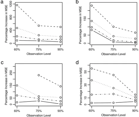
seem to vanish as the sample size increases. In order to point out the relative performances of the two approaches for estimating

θ

, we present four graphs inFig. 1for exponential and Weibull cases for configurations 11 and 23. Let MSEF

(θ)

denote the empirical mean square error for the estimator of

θ

using the full likelihood approach, and let MSEC

(θ)

θ

using the conditional likelihood approach. The vertical axes of all graphs inFig. 1give the percentage increase in mean square error when using

(9)

Table 2

Empirical mean square errors for 32 configurations. Exponential case, observation level 75%, n=180. The columnsτFandτC

contain the empirical values forτusing the full model and the conditional model, respectively, similar to other parameters. This notation is used in all the remaining tables.

Con. Model parameters Full likelihood Conditional likelihood

τ β θ ν γ τF βF θF νF γF τC βC θC 1 1 0.5 0.1 2 0.15 0.094 0.008 0.015 0.076 0.003 0.099 0.023 0.038 2 1 1 0.1 3.8 0.27 0.106 0.013 0.073 0.232 0.010 0.107 0.030 0.135 3 1 0.2 0.2 1.03 0.09 0.011 0.003 0.005 0.030 0.002 0.012 0.005 0.006 4 1 0.5 0.2 2 0.17 0.069 0.008 0.015 0.087 0.004 0.077 0.018 0.032 5 1 1 0.2 3.75 0.27 0.017 0.011 0.051 0.256 0.011 0.017 0.017 0.082 6 1 0.2 0.5 1.25 0.13 0.004 0.003 0.007 0.058 0.004 0.004 0.003 0.007 7 1 0.5 0.5 2.1 0.18 0.022 0.007 0.017 0.114 0.006 0.021 0.007 0.017 8 1 1 0.5 4 0.3 0.012 0.012 0.077 0.301 0.013 0.013 0.013 0.082 9 1 0.2 2 1.6 0.21 0.000 0.003 0.048 0.154 0.019 0.000 0.003 0.047 10 1 0.5 2 2.35 0.25 0.000 0.007 0.077 0.227 0.019 0.000 0.008 0.075 11 1 1 2 4.1 0.31 0.002 0.012 0.239 0.396 0.016 0.002 0.012 0.235 12 2 0.2 0.1 0.85 0.07 0.077 0.001 0.002 0.017 0.001 0.080 0.002 0.003 13 2 0.5 0.1 2 0.14 0.102 0.003 0.015 0.068 0.003 0.102 0.004 0.022 14 2 1 0.1 3.75 0.26 0.110 0.008 0.305 0.247 0.010 0.107 0.010 0.493 15 2 0.2 0.2 0.9 0.08 0.040 0.001 0.003 0.022 0.001 0.041 0.001 0.003 16 2 0.5 0.2 2 0.14 0.080 0.003 0.018 0.072 0.003 0.082 0.004 0.022 17 2 1 0.2 3.6 0.25 0.104 0.010 0.182 0.244 0.010 0.106 0.011 0.465 18 2 0.2 0.5 1 0.1 0.006 0.001 0.006 0.038 0.003 0.007 0.002 0.006 19 2 0.5 0.5 2 0.16 0.034 0.003 0.032 0.082 0.004 0.034 0.003 0.032 20 2 1 0.5 3.8 0.27 0.076 0.008 0.139 0.322 0.011 0.080 0.009 0.881 21 2 0.2 2 1.2 0.14 0.000 0.001 0.054 0.029 0.006 0.000 0.001 0.055 22 2 0.5 2 2 0.18 0.001 0.004 0.147 0.114 0.007 0.001 0.004 0.157 23 3 0.2 0.1 0.78 0.06 0.016 0.001 0.002 0.012 0.001 0.016 0.001 0.002 24 3 0.5 0.1 1.96 0.13 0.109 0.002 0.025 0.061 0.002 0.105 0.003 0.036 25 3 0.2 0.2 0.85 0.07 0.045 0.001 0.003 0.017 0.001 0.045 0.001 0.003 26 3 0.5 0.2 1.96 0.13 0.091 0.002 0.035 0.063 0.002 0.092 0.003 0.040 27 3 0.2 0.5 0.9 0.09 0.011 0.001 0.008 0.024 0.002 0.011 0.001 0.008 28 3 0.5 0.5 1.96 0.14 0.049 0.003 0.072 0.072 0.003 0.049 0.003 0.072 29 3 0.2 2 1 0.1 0.000 0.001 0.066 0.038 0.003 0.000 0.001 0.066 30 3 0.5 2 1.96 0.15 0.006 0.003 0.282 0.080 0.004 0.006 0.003 0.393 31 5 0.2 0.2 0.8 0.07 0.062 0.001 0.005 0.015 0.001 0.061 0.001 0.004 32 7 0.2 0.2 0.8 0.06 0.079 0.000 0.008 0.013 0.001 0.079 0.000 0.008 Table 3

Censoring and truncation parameters for different cases. Case Configuration Observation level

60% 75% 90% Exponential 5 ν 2.2 3.75 10 γ 0.48 0.27 0.1 11 ν 2.4 4.1 11 γ 0.57 0.31 0.12 23 ν 0.49 0.8 2.1 γ 0.107 0.062 0.023 27 ν 0.55 0.9 2 γ 0.15 0.086 0.03 Weibull 5 s 2 2 2 v 8 16 90 b 0.7 0.35 0.12 11 s 2 2 2 v 9.2 18.5 84 b 0.85 0.43 0.14 23 s 2 2 2 v 0.35 0.7 3.7 b 0.17 0.085 0.025 27 s 2 2 2 v 0.45 0.8 3.7 b 0.22 0.115 0.04

the conditional likelihood approach for estimating

θ

, instead of using the full likelihood approach. This can be considered as the cost of using the simpler conditional likelihood approach. We denote this quantity by PIMSEC

(θ)

, where

(10)

Table 4

Performances of the estimators, exponential case, Configurations 5 and 11, observation level 75%.

n Full likelihood Conditional likelihood

τF βF θF νF γF τC βC θC

Con. 5 (small jump) 60 bias 0.016 −0.032 0.266 −0.257 0.092 0.003 0.024 0.119

stdev 0.135 0.185 0.371 0.690 0.105 0.136 0.236 0.558 mse 0.019 0.035 0.209 0.542 0.020 0.019 0.056 0.326 100 bias 0.007 −0.036 0.194 −0.274 0.082 0.004 −0.004 0.108 stdev 0.129 0.144 0.276 0.525 0.077 0.131 0.179 0.395 mse 0.017 0.022 0.114 0.350 0.013 0.017 0.032 0.168 140 bias 0.007 −0.013 0.144 −0.337 0.088 −0.003 0.014 0.074 stdev 0.130 0.129 0.229 0.438 0.063 0.133 0.158 0.329 mse 0.017 0.017 0.073 0.306 0.012 0.018 0.025 0.113 180 bias 0.013 −0.010 0.109 −0.326 0.087 0.009 0.010 0.053 stdev 0.129 0.106 0.197 0.387 0.057 0.131 0.130 0.282 mse 0.017 0.011 0.051 0.256 0.011 0.017 0.017 0.082

Con. 11 (large jump) 60 bias 0.014 0.012 0.184 −0.332 0.114 0.017 0.012 0.487

stdev 0.077 0.198 0.368 0.613 0.126 0.079 0.209 0.918 mse 0.006 0.039 0.169 0.486 0.029 0.007 0.044 1.080 100 bias 0.009 0.003 0.115 −0.259 0.105 0.009 0.013 0.249 stdev 0.065 0.146 0.362 0.406 0.095 0.068 0.153 0.662 mse 0.004 0.021 0.144 0.232 0.020 0.005 0.024 0.500 140 bias 0.003 0.009 0.076 −0.386 0.103 0.004 0.011 0.137 stdev 0.050 0.127 0.349 0.470 0.067 0.051 0.129 0.510 mse 0.003 0.016 0.128 0.3709 0.015 0.003 0.017 0.279 180 bias 0.001 0.002 0.054 −0.221 0.0980 0.002 0.012 0.090 stdev 0.042 0.112 0.312 0.430 0.054 0.040 0.080 0.410 mse 0.002 0.013 0.100 0.234 0.013 0.002 0.007 0.176 Table 5

Performances of the estimators, exponential case, Configurations 23 and 27, observation level 75%.

Con. 23 (small jump) 60 bias 0.042 −0.003 0.022 −0.059 0.023 0.038 0.001 0.018

stdev 0.127 0.044 0.060 0.146 0.025 0.130 0.055 0.089 mse 0.018 0.002 0.004 0.025 0.001 0.018 0.003 0.008 100 bias 0.031 0.0001 0.017 −0.076 0.022 0.032 0.002 0.014 stdev 0.126 0.037 0.052 0.118 0.019 0.127 0.040 0.064 mse 0.017 0.001 0.003 0.020 0.001 0.017 0.002 0.004 140 bias 0.026 0.0001 0.013 −0.077 0.021 0.029 0.002 0.010 stdev 0.125 0.030 0.045 0.096 0.015 0.124 0.032 0.050 mse 0.016 0.001 0.002 0.015 0.001 0.016 0.001 0.003 180 bias 0.019 0.0003 0.009 −0.071 0.020 0.026 0.002 0.007 stdev 0.124 0.026 0.039 0.084 0.011 0.122 0.028 0.041 mse 0.016 0.001 0.002 0.012 0.001 0.016 0.001 0.002

Con. 27 (large jump) n=60 bias 0.044 0.002 0.075 −0.107 0.039 0.048 0.003 0.070

stdev 0.186 0.052 0.160 0.184 0.037 0.188 0.053 0.160 mse 0.037 0.003 0.031 0.045 0.003 0.038 0.003 0.030 n=100 bias 0.027 0.003 0.041 −0.123 0.038 0.029 0.004 0.036 stdev 0.149 0.039 0.123 0.141 0.027 0.149 0.040 0.123 mse 0.023 0.002 0.017 0.035 0.002 0.023 0.002 0.016 n=140 bias 0.017 0.005 0.025 −0.120 0.037 0.019 0.006 0.019 stdev 0.119 0.034 0.095 0.116 0.023 0.120 0.034 0.095 mse 0.014 0.001 0.010 0.028 0.002 0.015 0.001 0.009 n=180 bias 0.011 0.004 0.020 −0.117 0.037 0.012 0.005 0.015 stdev 0.104 0.029 0.086 0.101 0.020 0.105 0.029 0.087 mse 0.011 0.001 0.008 0.024 0.002 0.011 0.001 0.008

The horizontal axes of the graphs inFig. 1represent the observation levels, 60%, 75% and 90%. Each graph gives the profiles of PIMSEC

(θ)

for three observation levels for sample sizes 60, 100, 140 and 180. The results indicate that the cost of using the conditional model can be very high, but this remarkable cost vanishes fast as the sample size increases. Recall thatFig. 1

reports the comparisons for estimating

θ

, where the conditional likelihood approach has the poorest performance. For the other model parameters the two methods are very similar. Note that when the observation level is 60% and when n

=

60,

(11)

a

b

c

d

Fig. 1. Comparison of full likelihood model and conditional likelihood model via PIMSEC(θ). (a) Exponential case, configuration 11, (b) Exponential case,

configuration 23, (c) Weibull case, configuration 11, (d) Weibull case, configuration 23. Sample sizes are n=60 (− − −), n=100 (· · ·), n=140 (—·—) and n=180 (—).

a

b

Fig. 2. (a) Under misspecification, comparison of full model and conditional model via PIMSEC(θ). (b) Comparison of correct specification and

misspecification via PIMSEF,E(θ). Sample sizes are n=60 (− − −), n=100 (· · ·), n=140 (—·—) and n=180 (—).

we do not have results inFig. 1-c. This is because at this level our optimization routines in the full likelihood model did not lead to a solution, which was noted earlier as a disadvantage of the full likelihood model.

5.3. The effect of model misspecification

In order to address the issue regarding the effect of model misspecification in the full likelihood approach, we carried out two simulation studies where the data are generated from configuration 11 and Weibull case with the parameters given inTable 3. In the first study we compared the full likelihood model which falsely assumes exponential distribution for the censoring and truncation variables with the conditional likelihood model. In the second study we compared the full likelihood model which falsely assumes exponential distribution with the one that correctly assumes Weibull distribution.

Fig. 2-a reports the results for the first study, where the graph is designed similar to the graphs inFig. 1with PIMSEC

(θ)

on the vertical axis. Note that this graph is comparable withFig. 1-c, and the decrease in the PIMSEC

(θ)

values indicate the importance of model misspecification. When n

=

180 the conditional approach performs better.

(12)

Fig. 2-b reports the results for the second study for illustrating the disadvantages of model misspecification. Let MSEF,E

(θ)

θ

using the exponential full likelihood model, and let MSEF,W

(θ)

θ

using the Weibull full likelihood model. Define

PIMSEF,W

(θ) =

100

× [

MSEF,W

(θ) −

MSEF,E

(θ)]/

MSEF,E

(θ).

The vertical axis ofFig. 2-b is the PIMSEF,W

(θ)

, where negative values indicate the importance of model misspecification. The results show that PIMSEF,W

(θ)

can get as low as

−

50 indicating that the correct specification performs much better. In summary,Fig. 2provides some evidence that the full likelihood model is not robust to misspecification of the model.

6. Summary and conclusions

In this paper we considered piecewise constant hazard functions with a single unknown change-point, when the observations are subject to random left truncation and right censoring. We discussed two maximum likelihood estimation procedures, namely, the full likelihood method and the conditional likelihood method. The full likelihood method assumes parametric families of distributions for the censoring and truncation variables. This complicates the model to some extent, as the number of parameters to be estimated increase, and the lack of closed form maximum likelihood estimators forces one to use numerical optimization techniques. If the distributional assumptions are accurate, this fully parametric model is expected to produce good estimators. The conditional likelihood method does not make any distributional assumptions and focuses only on estimating the three model parameters of the hazard function. Its simpler structure allows the conditional likelihood method to provide closed form estimators for the model parameters. However, it can have large bias and variance especially for small sample sizes, since it constructs the censoring and truncation component of the likelihood function solely on the observed values.

Our numerical studies indicate that both methods can easily be implemented and their performances are good. When the distributional assumptions of the full likelihood method are correct, the performances of the two methods are close for estimating the location of the change-point and the initial hazard rate, but for estimating the size of the change, the full likelihood method performs better. We observed that this difference tends to vanish as the sample size increases. Another important finding of the study is that the full likelihood model is not robust to model misspecification, and in some cases it is outperformed by the conditional likelihood model.

Appendix

Here we present the results of the numerical study discussed in Section5in more detail. We report Configurations 11 and 23 as representatives of large jump and small jump cases, respectively.Tables 6and7report the exponential case for observation levels 60% and 90%. Note that a 75% observation level is given in Section5.Tables 8–10report the Weibull case for observation levels 60%, 75% and 90%.

Table 6

Performance of the estimators, exponential case, Configurations 11 and 23, observation level 60%.

Con. 11 (large jump) 60 bias 0.022 0.091 0.184 −0.844 0.308 0.032 0.111 0.654

stdev 0.081 0.224 0.378 0.509 0.132 0.084 0.250 1.345 mse 0.007 0.058 0.177 0.971 0.112 0.008 0.075 2.237 100 bias 0.012 0.068 0.118 −0.731 0.282 0.020 0.119 0.288 stdev 0.069 0.171 0.376 0.283 0.078 0.072 0.209 0.871 mse 0.005 0.034 0.149 0.614 0.086 0.006 0.058 0.842 140 bias 0.008 0.059 0.107 −0.798 0.335 0.012 0.108 0.158 stdev 0.055 0.142 0.367 0.194 0.098 0.058 0.173 0.657 mse 0.003 0.024 0.146 0.674 0.122 0.004 0.042 0.457 180 bias 0.005 0.051 0.099 −0.712 0.313 0.008 0.101 0.084 stdev 0.044 0.132 0.351 0.179 0.068 0.046 0.156 0.492 mse 0.002 0.020 0.133 0.539 0.103 0.002 0.035 0.249

Con. 23 (small jump) 60 bias 0.038 0.011 0.021 −0.178 0.069 0.033 0.033 −0.011

stdev 0.135 0.051 0.064 0.128 0.045 0.136 0.082 0.122 mse 0.020 0.003 0.005 0.048 0.007 0.020 0.008 0.015 100 bias 0.027 0.005 0.016 −0.145 0.065 0.023 0.028 −0.013 stdev 0.131 0.041 0.057 0.065 0.030 0.138 0.062 0.090 mse 0.018 0.002 0.004 0.025 0.005 0.020 0.005 0.008 140 bias 0.020 0.016 0.011 −0.191 0.067 0.022 0.030 −0.015 stdev 0.127 0.038 0.051 0.088 0.029 0.132 0.050 0.072 mse 0.017 0.002 0.003 0.044 0.005 0.018 0.003 0.005 180 bias 0.016 0.005 0.008 −0.171 0.060 0.020 0.026 −0.015 stdev 0.120 0.030 0.046 0.074 0.025 0.130 0.044 0.061 mse 0.015 0.001 0.002 0.035 0.004 0.017 0.003 0.004

(13)

Table 7

Performance of the estimators, exponential case, Configurations 11 and 23, observation level 90%.

Con. 11 (large jump) 60 bias 0.013 0.001 0.154 0.012 0.016 0.013 −0.005 0.444

stdev 0.074 0.172 0.377 1.302 0.059 0.076 0.174 0.892 mse 0.006 0.030 0.166 1.695 0.004 0.006 0.030 0.993 100 bias 0.006 −0.001 0.110 0.007 0.016 0.006 −0.004 0.228 stdev 0.061 0.128 0.369 1.135 0.046 0.061 0.129 0.627 mse 0.004 0.016 0.148 1.288 0.002 0.004 0.017 0.445 140 bias 0.002 −0.001 0.085 −0.039 0.015 0.002 −0.003 0.157 stdev 0.052 0.114 0.342 0.988 0.037 0.052 0.114 0.499 mse 0.003 0.013 0.124 0.978 0.002 0.003 0.013 0.274 180 bias 0.001 −0.001 0.062 0.003 0.014 0.002 −0.002 0.112 stdev 0.044 0.103 0.334 0.879 0.031 0.047 0.096 0.392 mse 0.002 0.011 0.115 0.773 0.001 0.002 0.009 0.166

Con. 23 (small jump) 60 bias 0.033 −0.006 0.021 0.001 0.004 0.030 −0.005 0.023

stdev 0.131 0.039 0.058 0.299 0.011 0.131 0.043 0.076 mse 0.018 0.002 0.004 0.089 0.0001 0.018 0.002 0.006 100 bias 0.034 −0.005 0.016 0.004 0.003 0.032 −0.004 0.017 stdev 0.126 0.031 0.049 0.244 0.008 0.127 0.032 0.056 mse 0.017 0.001 0.003 0.060 0.0001 0.017 0.001 0.003 140 bias 0.022 −0.003 0.015 −0.012 0.003 0.023 −0.004 0.015 stdev 0.125 0.027 0.044 0.199 0.007 0.125 0.027 0.046 mse 0.016 0.001 0.002 0.040 0.0001 0.016 0.001 0.002 180 bias 0.019 −0.002 0.014 0.005 0.002 0.017 −0.003 0.013 stdev 0.124 0.025 0.040 0.181 0.005 0.121 0.024 0.041 mse 0.016 0.001 0.002 0.033 0.0001 0.015 0.001 0.002 Table 8

Performance of the estimators, Weibull case, Configurations 11 and 23, observation level 60%.

τF βF θF sF vF bF τC βC θC

Con. 11 (large jump) 100 bias 0.012 −0.006 0.310 0.022 0.376 0.008 0.011 −0.008 0.468

stdev 0.071 0.157 0.597 0.148 1.768 0.127 0.071 0.157 0.957 mse 0.005 0.025 0.453 0.022 3.267 0.016 0.005 0.025 1.135 140 bias 0.005 −0.016 0.223 0.009 0.221 0.003 0.006 −0.017 0.303 stdev 0.057 0.134 0.548 0.128 1.589 0.113 0.059 0.134 0.714 mse 0.003 0.018 0.350 0.016 2.574 0.013 0.004 0.018 0.602 180 bias 0.003 −0.008 0.180 0.004 0.112 0.001 0.003 −0.015 0.181 stdev 0.045 0.119 0.551 0.110 1.472 0.096 0.049 0.118 0.602 mse 0.002 0.014 0.336 0.012 2.179 0.009 0.002 0.014 0.395

Con. 23 (small jump) 60 bias 0.030 −0.016 0.046 0.046 0.006 0.002 0.031 −0.009 0.034

stdev 0.132 0.046 0.072 0.226 0.075 0.036 0.131 0.057 0.099 mse 0.018 0.002 0.007 0.053 0.006 0.001 0.018 0.003 0.011 100 bias 0.024 −0.010 0.029 0.024 0.004 0.001 0.021 −0.006 0.022 stdev 0.130 0.037 0.059 0.160 0.054 0.028 0.130 0.042 0.074 mse 0.017 0.001 0.004 0.026 0.003 0.001 0.017 0.002 0.006 140 bias 0.021 −0.007 0.021 0.016 0.003 0.001 0.020 −0.006 0.020 stdev 0.125 0.033 0.054 0.139 0.046 0.023 0.125 0.035 0.059 mse 0.016 0.001 0.003 0.020 0.002 0.001 0.016 0.001 0.004 180 bias 0.018 −0.002 0.014 0.010 0.002 0.001 0.018 −0.005 0.019 stdev 0.121 0.030 0.051 0.117 0.038 0.021 0.121 0.028 0.050 mse 0.015 0.001 0.003 0.014 0.001 0.0001 0.015 0.001 0.003

(14)

Table 9

Con. 11 (large jump) 60 bias 0.004 −0.009 0.233 0.011 0.574 −0.003 0.007 −0.014 0.503

stdev 0.081 0.198 0.572 0.131 2.843 0.110 0.082 0.198 1.005 mse 0.007 0.039 0.381 0.017 8.412 0.012 0.007 0.039 1.263 100 bias 0.007 −0.006 0.203 0.026 1.233 −0.007 0.008 −0.007 0.275 stdev 0.070 0.148 0.543 0.130 3.537 0.068 0.070 0.148 0.692 mse 0.005 0.022 0.336 0.018 14.031 0.005 0.005 0.022 0.554 140 bias 0.008 −0.005 0.184 −0.006 −0.149 0.005 0.008 −0.006 0.231 stdev 0.051 0.120 0.501 0.080 1.659 0.073 0.052 0.120 0.603 mse 0.003 0.014 0.285 0.006 2.774 0.005 0.003 0.014 0.417 180 bias 0.007 −0.004 0.170 −0.002 −0.121 0.003 0.004 −0.005 0.205 stdev 0.042 0.095 0.472 0.060 1.974 0.054 0.041 0.102 0.531 mse 0.002 0.009 0.252 0.004 3.911 0.003 0.002 0.010 0.324

stdev 0.128 0.042 0.067 0.217 0.119 0.022 0.130 0.049 0.087 mse 0.019 0.002 0.006 0.050 0.014 0.0001 0.019 0.002 0.009 100 bias 0.024 −0.008 0.025 0.026 0.007 0.001 0.020 −0.006 0.021 stdev 0.128 0.034 0.053 0.159 0.086 0.018 0.129 0.037 0.062 mse 0.017 0.001 0.003 0.026 0.007 0.0001 0.017 0.001 0.004 140 bias 0.017 −0.007 0.020 0.019 0.007 0.002 0.016 −0.006 0.018 stdev 0.123 0.029 0.047 0.138 0.074 0.015 0.124 0.031 0.052 mse 0.015 0.001 0.003 0.019 0.006 0.0001 0.016 0.001 0.003 180 bias 0.010 −0.004 0.018 0.011 0.005 0.001 0.008 −0.005 0.011 stdev 0.105 0.021 0.041 0.121 0.069 0.014 0.116 0.028 0.044 mse 0.011 0.0001 0.002 0.015 0.005 0.0001 0.014 0.001 0.002 Table 10

Con. 11 (large jump) 60 bias 0.009 −0.015 0.273 0.012 2.498 −0.001 0.011 −0.016 0.427

(15)

References

Antoniadis, A., Gijbels, I., MacGibbon, B., 1998. Nonparametric estimation for the location of a change-point in an otherwise smooth hazard function under random censoring. Tech. Report. Institute of Statist. U.C.L., Louvain-La-Neuve.

Byrd, R.H., Lu, P., Nocedal, J., Zhu, C., 1995. A limited memory algorithm for bound constrained optimization. SIAM Journal on Scientific Computing 16, 1190–1208.

Dupuy, J.-F., 2009. Detecting change in a hazard regression model with right-censoring. Journal of Statistical Planning and Inference 139, 1578–1586. Frobish, D., Ebrahimi, N., 2009. Parametric estimation of change-points for actual event data in recurrent events models. Computational Statistics and Data

Analysis 53, 671–682.

Gijbels, I., Gürler, Ü., 2003. Estimation of a change-point in a hazard function based on censored data. Lifetime Data Analysis 9, 395–411.

Gijbels, I., Wang, J.-L., 1993. Strong representations of the survival function estimator for truncated and censored data with applications. Journal of Multivariate Analysis 47, 210–229.

Goodman, M.S., Li, Y., Tiwari, R.C., 2006. Survival Analysis with Change Point Hazard Functions. Harvard University Biostatistics Working Paper Series, Paper 40.

Hudgens, M.G., Satten, G.A., Longini Jr., M.I., 2001. Nonparametric maximum likelihood estimation for competing risks survival data subject to interval censoring and truncation. Biometrics 57, 74–80.

Hyde, J., 1977. Testing survival under right censoring and left truncation. Biometrika 64, 225–230.

Kalbfleisch, J.D., Lawless, J.F., 1989. Inference based on retrospective ascertainment: an analysis of the data on transfusion-related AIDS. Journal of the American Statistical Association 84, 360–372.

Karasoy, D.S., Kadılar, C., 2007. A new Bayes estimate of the change-point in the hazard function. Computational Statistics and Data Analysis 51, 2993–3001. Klein, J.P., Moeschberger, M.L., 2003. Survival Analysis, second ed. Springer, New York.

Lim, H., Sun, J., Matthews, D.E., 2002. Maximum likelihood estimation of a survival function with a change-point for truncated and interval-censored data. Statistics in Medicine 21, 743–752.

Liu, M., Lu, W., Shao, Y., 2008. A Monte Carlo approach for change-point detection in the Cox proportional hazards model. Statistics in Medicine 27, 3894–3909.

Loader, C.R., 1991. Inference for hazard rate change-point. Biometrika 78, 835–843.

Luo, X., Turnbull, B.W., Clark, L.C., 1997. Likelihood ratio tests for a change-point with survival data. Biometrika 84, 555–565. Matthews, D.E., Farewell, V.T., 1982. On testing for a constant hazard against a change-point alternative. Biometrics 38, 463–468.

Pan, W., Chappell, R., 1998. Computation of the NPMLE of distribution functions for interval censored and truncated data with applications to the Cox model. Computational Statistics and Data Analysis 28, 33–50.

Pham, T.D., Nguyen, H.T., 1993. Bootstrapping the change-point of a hazard rate. Annals of the Institute of Statistical Mathematics 45, 331–340. Tsai, W., Jewell, N., Wang, M.-C., 1987. A note on the product-limit estimator under right censoring and left truncation. Biometrika 74, 883–886. Turnbull, B.W., 1976. The empirical distribution function with arbitrarily grouped, censored and truncated data. Journal of the Royal Statistical Society:

Series B 38, 290–295.