Financial, economic, banking sector and institutional development and productivity

(1)

(2)

(3)

FINANCIAL, ECONOMIC, BANKING

SECTOR AND INSTITUTIONAL

DEVELOPMENT AND PRODUCTIVITY

The Institute of Economics and Social Sciences of

Bilkent University by

G ÖKÇ E ÖZCAN

In Partial Fulfilment of the Requirements for the Degree of

MASTER OF ARTS in

THE DEPARTMENT OF ECONOMICS BILKENT UNIVERSITY

ANKARA November 2004

(4)

I certify that I have read this thesis and have found that it is fully adequate, in scope and in quality, as a thesis for the degree of Master of Arts in Economics.

Associate Professor Fatma Ta¸skın Supervisor

I certify that I have read this thesis and have found that it is fully adequate, in scope and in quality, as a thesis for the degree of Master of Economics.

Assistant Professor ¨Umit ¨Ozlale Examining Committee Member

I certify that I have read this thesis and have found that it is fully adequate, in scope and in quality, as a thesis for the degree of Master of Economics.

Assistant Professor Zeynep ¨Onder Examining Committee Member

Approval of the Institute of Economics and Social Sciences Professor Erdal Eren

(5)

ABSTRACT

FINANCIAL, ECONOMIC, BANKING SECTOR AND INSTITUTIONAL DEVELOPMENT AND PRODUCTIVITY

¨

Ozcan, G¨ok¸ce

Masters of Arts, Department of Economics Supervisor: Fatma Ta¸skın

November 2004

This thesis explores the links between Malmquist Productivity Index (and its two components, namely efficiency change and technological change) and the banking sector, economic, financial development and institutional variables. Re-sults show that there is a positive link between the banking, economic and financial variables and the productivity indexes. Also, data show that cross-country dif-ferences in legal and accounting systems play significant role in the improvement of the productivity indexes- Malmquist Index and its two components, efficiency change and technical change.

(6)

¨ OZET

F˙INANSAL, EKONOM˙IK, BANKACILIK SEKT ¨OREL VE KURUMSAL GEL˙IS¸˙IM VE ¨URETKENL˙IK

¨

Ozcan, Gök¸ce Mastır, ˙Iktisat Bölümü Tez Yöneticisi: Fatma Ta¸skın

Eyl¨ul 2004

Bu tez, Malmquist Üretkenlik Göstergesi (ve bu göstergenin iki bile¸seni olan verimlilik deˇgi¸simi ve teknolojik deˇgi¸sim) ile bankacılık sektörü, ekonomik, fi-nansal ve kurumsal deˇgi¸simin arasındaki ili¸skiyi incelemektedir. Sonu¸clar göstermi¸stir ki, bankacılık, ekonomik, finansal ve de kurumsal deˇgi¸skenler ile bu üretkenlik göstergeleri arasında pozitif bir ili¸ski vardır. Ayrıca, veriler ülkeler arası kanuni ve muhasebe sistemleri arasındaki farkların bu üretkenlik göstergelerinin geli¸siminde belirgin bir rol oynadıˇgını sergilemi¸stir.

(7)

ACKNOWLEDGEMENTS

Although this thesis is the output of my studies at Bilkent University Eco-nomics Department Graduate Program, it is certain that all my previous educa-tion helped in some ways to complete this thesis. Therefore, I would like to thank everybody who has had a contribution in this journey; my teachers, my friends, and especially to my family for their endless support.

However, if I have to name one person to acknowledge here, that would defi-nitely be Fatma Ta¸skın, my supervisor in this study. Her assistance and support - both academically and personally- have been the most important factor for me to finish this thesis and get my degree. I consider myself very lucky since I have had the chance to work with her and get to know her.

(8)

1 INTRODUCTION

Relationship between better functioning financial structure - the mix of financial contracts, markets and institutions- and economic growth has been subject to many research papers. Do well functioning financial structure (stock markets, banks, legal environment) promote long-run growth? Economists hold different opinions regarding the importance of the financial structure for economic growth. Researchers who claim that well functioning financial structure promote long-run growth argue that with the help of debt contracts and financial intermediaries, economic agents ameliorate the economic consequences of informational asymme-tries and they provide proper resource allocation. On the other hand, researchers who claim that finance is a relatively unimportant factor in economic development argue that higher returns from better resource allocation may depress saving rates enough such that overall growth rates actually slow with enhanced financial de-velopment.

1.1 Supporters of the View

Hamilton (1789) argued that ”banks were the happiest engines that ever were invented” for spurring economic growth. Schumpeter (1912) argues that finan-cial intermediaries are essential for technological innovation and economic de-velopment since they help mobilizing savings, evaluating projects, monitoring managers, managing risks, and facilitating transactions. Schumpeter (1912) also states that well-functioning banks spur technological innovation by identifying and funding the entrepreneurs with the best chances of successfully implementing innovative products and production processes. Bagehot (1873) and Hicks (1969) say that financial system played a crucial role in igniting industrialization in Eng-land by facilitating the mobilization of capital for ”immense works”. Goldsmith

(12)

(1969) and McKinnon (1973) empirically show the close relationship between fi-nancial and economic development for a few countries.

Besides the historical focus on banking, there is an expanding theoretical lit-erature on the links between stock markets and long-run growth. Levine (1991) and Bencivenga (1991) et al. show models where more liquid stock markets de-crease the propensity not to invest in long-duration projects because investors can sell their stocks before the project matures if they need their savings. Therefore, liquidity facilitates investment in longer-run, higher-return projects that boost productivity growth.

Similar consequences are obtained by Devereux (1994) et al. and Obstfeld (1994) about stock markets in the existence of greater international risk shar-ing through internationally integrated stock markets . Greater international risk sharing induces a portfolio shift from safe, low-return investments to high-return investments, thereby accelerating productivity growth.

1.2 Supporters of the Opposing View

In contrast to the idea that financial structure and economic growth are linked, there is support for the opposing view that finance is a relatively unimportant factor in economic development.

Adams (1819) states that banks harm the ”morality, tranquility, and even wealth” of nations. Lucas (1988) argues that the ties between financial and eco-nomic development is ”badly over-stressed”. The debate also exists about whether greater stock market liquidity actually encourages a shift to higher-return projects that stimulate productivity growth. Since more liquidity makes it easier to sell shares, some argue that more liquidity reduces the incentives of shareholders to undertake the costly task of monitoring managers (Shleifer (1986) et al.; Bhide (1993)). In turn, weaker corporate governance impedes effective resource alloca-tion and slows productivity growth.

(13)

1.3 Purpose of the Paper

In the view of the papers stated above, the objective of the paper is to ad-dress the question of economic growth and financial development from another perspective. Traditionally, real per capita GDP growth or real per capita cap-ital stock growth have been used as a dependent variable. This paper replaces economic growth with a specific productivity measure, Malmquist index intro-duced by Fare et al (1994). The index is further decomposed into two component measures, efficiency change (diffusion) and technical change (innovation). The paper examines the role of banking, financial, economic and institutional factors on the development of the above productivity measures. The empirical analysis is conducted on a group of countries, which includes developed and developing coun-tries. Most of the OECD countries (with the exception of Mexico and Turkey) are included in the first group. The developing countries are selected from a group of countries, which had some financial liberalization and reform experience. Panel data approach is utilized to expose the relationship between the produc-tivity and efficiency measures and the indicators of banking, financial, economic and institutional factors.

The plan of the study is as follows: Section two describes the Malmquist productivity index measures, section three gives details of data and methodology, section four reports the empirical results and section five concludes.

(14)

2 MALMQUIST PRODUCTIVITY INDEX

2.1 Description of Malmquist Productivity Index

In this study a Malmquist index introduced by Fare et al. (1994) is used to measure the productivity growth between two groups of countries (developed and developing countries). To define the Malmquist index of productivity change, it is assumed that for each time period t = 1, ..., T , the production technology St _{models the transformation of inputs, x}t _{∈ R}N

+, into outputs, yt ∈ RM+. In

mathematical representation this can be expressed as:

St_{= {(x}t_{, y}t_{) : x}t _{can produce y}t_} ₍₁₎

The output distance function at t is defined as:

D0(xt, yt) = inf {θ : (xt, yt/θ) ∈ St} (2)

= (sup{θ : (xt_{, y}t_{/θ) ∈ S}t_})−1 ₍₃₎

This function is defined as the reciprocal of the ”maximum” proportional expansion of the output vector yt_{, given inputs x}t_{. Output distance function is}

equal to one if and only if (xt_{, y}t_{) is on the boundary or frontier of technology. In}

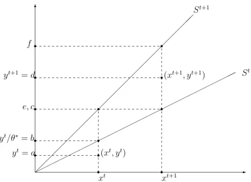
our calculations, the country with the distance function equal to one constructs the best practice world frontier and the distance of individual countries is computed according to this world frontier. This is illustrated in Figure 1. In the figure, observed production at t is interior to the boundary of technology at t, so (xt_{, y}t_{) is}

not technically efficient. The distance function gives the reciprocal of the greatest proportional increase in outputs given inputs, such that output is still feasible. In

(15)

distance function for our observation in terms of distances on the y-axis is 0a/0b, which is less than 1.

-6 ©©©© ©©©© ©©©© ©©©© ©©©© ©©©© ©©©© ¡¡ ¡¡ ¡¡ ¡¡ ¡¡ ¡¡ ¡¡ ¡¡ ¡¡ ¡¡ ¡¡ r r r r r r r r r r r r r xt _xt+1 yt_{= a} yt_/θ∗ _{= b} e, c yt+1_{= d} f (xt_{, y}t₎ (xt+1_{, y}t+1₎ St St+1

Figure 1 - The Malmquist Output-Based Index of Total Factor Productivity and Output Distance Function

To define the Malmquist index, one needs to define distance functions with re-spect to two different time periods such as Dt

0(xt+1, yt+1) = inf {θ : (xt+1, yt+1/θ) ∈

St_{}. This distance function measures the maximal proportional change in outputs}

required to make (xt+1_{, y}t+1_{) feasible in relation to the technology at t. Similarly,}

distance function that measures the maximal proportional change in output re-quired to make (xt_{, y}t_{) feasible in relation to the technology at t + 1 is given as}

Dt+1

0 (xt, yt) = inf {θ : (xt, yt/θ) ∈ St+1}.

Malmquist productivity index is defined in two different ways depending on whether period t or period t + 1 is the reference technology:

Mt₌ Dt+10 (xt+1, yt+1) Dt 0(xt, yt) or Mt+1₌ D0t+1(xt+1, yt+1) Dt+1 0 (xt, yt) . (4)

In order to avoid choosing arbitrary benchmark, Malmquist productivity change index is defined as the geometric mean of the two type indexes given above:

Mt 0(xt+1, yt+1, xt, yt) = " Dt+1 0 (xt+1, yt+1) Dt 0(xt, yt) Dt+1 0 (xt+1, yt+1) Dt+1 0 (xt, yt) #_1/2 (5)

(16)

Equivalent way of writing this expression is Mt 0(xt+1, yt+1, xt, yt) = Dt+1 0 (xt+1, yt+1) Dt 0(xt, yt) " Dt 0(xt+1, yt+1) Dt+1₀ (xt+1_{, y}t+1₎ Dt 0(xt, yt) Dt+1₀ (xt_{, y}t₎ #_1/2 (6)

where the ratio outside the brackets measures the change in relative efficiency (i.e., is from maximum potential production) between years t and t + 1. The geo-metric mean of the two ratios inside the brackets captures the shift in technology between the two periods evaluated at xt _{and x}t+1_{. In this expression, efficiency}

change is given as:

Dt+1

0 (xt+1, yt+1)

Dt

0(xt, yt)

(7) and technical change is given as:

" Dt 0(xt+1, yt+1) Dt+1 0 (xt+1, yt+1) Dt 0(xt, yt) Dt+1 0 (xt, yt) #_1/2 . (8)

For values greater than one, efficiency change component will indicate that the country has improved its relative technical efficiency during the period considered and experienced diffusion of technology. Technical change component measures the shift in frontier between two periods. A value greater than one will indicate that there is technical progress along the input and output mix of the country. The Malmquist index, which displays the changes in the productivity, is the prod-uct of these measures. While index values greater than one show improvement in the productivity over time, values smaller than one indicate deterioration in performance.

The decomposition is illustrated in Figure 1 where technical advance has oc-curred between the years t and t + 1. In terms of the distances along the y-axis, the Malmquist Index becomes

M0(xt+1, yt+1, xt, yt) = µ 0d 0f ¶µ 0b 0a ¶"µ 0d/0e 0d/0f ¶µ 0a/0b 0a/0c ¶#1/2 (9) = µ 0d 0f ¶µ 0b 0a ¶"µ 0f 0e ¶µ 0c 0b ¶#1/2 (10)

(17)

2.2 Calculation of Malmquist Productivity Index

In our study, Malmquist productivity index is calculated by using non-parametric programming techniques. The aggregate output measure is GDP of the countries between years 1970 − 1991, input measures are capital and labor. These values are compiled from The Penn World Tables (2002).

In our model, we assume that there are k = 1, 2, ..., K countries using n = 1, 2, ..., N inputs, xk,t

n , at each time period t = 1, 2, ..., T . These inputs produce

m = 1, 2, ..., M outputs, yk,t

m. In the model we assume that capital and labor are

the input variables and the GDP of each country is our output value. The reference technology in period t is constructed from the data set as:

St₌          (xt_{, y}t_{) : y}t m ≤ P_K k=1zk,tyk,t m = 1, ..., M P_K k−1zk,txk,tn n = 1, ..., N zk,t _{≥ 0} _{k = 1, ..., K}          where constant returns to scale is assumed.

There are four different linear programming problems to calculate the produc-tivity of a country between years t and t + 1:

1)Dt

0(xt, yt), 2)Dt+10 (xt+1, yt+1), 3)Dt0(xt+1, yt+1), 4)Dt+10 (xt, yt) . So for each

k0 _{= 1, ..., K these four linear programming problem can be defined as:}

1) ³ D₀t(xk0,t, yk0,t) ´₋₁ =                        max θk0 subject to θk0 yk0_,t m ≤ P_K k=1zk,tyk,tm m = 1, ..., M P_K k=1zk,txk,tn ≤ xk 0_,t n n = 1, ..., N zk,t _{≥ 0} _{k = 1, ..., K} 2) ³ D₀t+1(xk0,t+1, yk0,t+1) ´₋₁ =                        max θk0 subject to θk0 yk0_,t+1 m ≤ P_K k=1zk,t+1yk,t+1m m = 1, ..., M P_K k=1zk,t+1xk,t+1n ≤ xk 0_,t+1 n n = 1, ..., N zk,t+1 _{≥ 0} _{k = 1, ..., K}

(18)

3) ³ Dt₀(xk0,t+1, yk0,t+1) ´₋₁ =                        max θk0 subject to θk0 yk0_,t+1 m ≤ P_K k=1zk,tymk,t m = 1, ..., M P_K k=1zk,txk,tn ≤ xk 0_,t+1 n n = 1, ..., N zk,t _{≥ 0} _{k = 1, ..., K} 4) ³ D₀t+1(xk0,t, yk0,t) ´₋₁ =                        max θk0 subject to θk0 yk0_,t m ≤ P_K k=1zk,t+1ymk,t+1 m = 1, ..., M P_K k=1zk,t+1xk,t+1n ≤ xk 0_,t n n = 1, ..., N zk,t+1 _{≥ 0} _{k = 1, ..., K}

In order to find out the Malmquist productivity index, we need to solve the above equations.

(19)

3 DATA AND METHODOLOGY

As mentioned above, the countries are grouped into 2 groups, which are developed countries (Canada, U.S.A., Japan, Austria, Belgium, Denmark, Finland, France, Germany, Ireland, Italy, Norway, Spain, Sweden, U.K., Australia) and developing countries (Nigeria, Zimbabwe, Mexico, Argentina, Chile, Venezuela, India, Korea, Greece, Turkey, Philippines, Taiwan, Thailand, Colombia). For these countries, Malmquist productivity index and its components, efficiency change index and technical change index are calculated. In order to find these indexes, the equations defined above need to be solved. These equations are solved by using GAMS (General Algebraic Modeling System (2002)) for each time period between 1970 and 1990. So for each country, we need to solve 61 linear programming problems, which makes totally 30 ∗ 61 = 1830 problems. The Malmquist productivity index and its components are the dependent variables of our regression models.

Regressors, on the other hand, are grouped into 4 groups. Banking develop-ment variables include claims on governdevelop-ment, claims on private sector, domestic credit provided by banking sector, domestic credit growth rate, financing from abroad, gross private capital flows, liquid liabilities, credit to private sector, total domestic financing. Economic variables are total central government debt, foreign direct investment-net inflows (% of GDP), foreign direct investment-net inflows (% of gross capital formation), gross capital formation growth, GDP growth, gross capital formation, inflation-consumer prices, inflation-GDP deflator, initial per capita income, openness, per capita GNP growth, real interest rate, tax rev-enue, unemployment. Financial sector variables are defined as listed domestic companies, market capitalization of listed companies, portfolio investment-bonds, portfolio investment-equity, turnover ratio of stocks traded, total value of stocks traded. Finally institutional variables are accounting standards, creditor rights,

(20)

enforcement of contracts, coefficient of education efficiency, illiteracy rate, re-search and development expenditures. The detailed explanation of these variables is given in Chapter 4. These data are compiled from World Bank’s ”World Devel-opment Indicators” (2000) and IMF’s ”International Financial Statistics” (2002). Some of the institutional variables such as accounting standards, creditor rights and enforcement of contracts have been directly taken from Levine et al (2000).

(21)

4 DESCRIPTION OF THE VARIABLES

4.1 Banking Development Variables

Since banking sector constitutes a very important part of the financial sector of a country, we believe that productivity measures (Malmquist index and its two components- efficiency change and technical change) and the efficiency of the banking sector are closely related. Data regarding the banking sector variables are taken from World Bank’s ”World Development Indicators” Database (2000). The variables that are classified as banking sector variables and the descriptions are:

4.1.1 Claims on Governments (claimgov )

claimgov include the claims on governments and other public entities (this corresponds to IFS line 32an + 32b + 32bx + 32c) that usually comprise direct credit for specific purposes such as financing of the government budget deficit or loans to state enterprises, advances against future credit authorizations, and purchases of treasury bills and bonds, net of deposits by the public sector. Public sector deposits with the banking system also include sinking funds for the service of debt and temporary deposits of government revenues. Money and quasi money (M2) comprise the sum of currency outside banks, demand deposits other than those of the central government, and the time, savings, and foreign currency deposits of resident sectors other than the central government. The data are given as annual growth as percentage of M2.

(22)

4.1.2 Claims on Private Sector (claimpriv )

Claims on private sector (IFS line 32d (2002)) include gross credit from the financial system to individuals, enterprises, nonfinancial public entities not in-cluded under net domestic credit, and financial institutions not inin-cluded else-where. Money and quasi money (M2) comprise the sum of currency outside banks, demand deposits other than those of the central government, and the time, savings, and foreign currency deposits of resident sectors other than the central government. The data are given as annual growth as percentage of M2.

4.1.3 Domestic Credit Provided by Banking Sector (dcredbybank ) Domestic credit provided by the banking sector includes all credit to various sectors on a gross basis, with the exception of credit to the central government, which is net. The banking sector includes monetary authorities and deposit money banks, as well as other banking institutions where data are available (including institutions that do not accept transferable deposits but do incur such liabilities as time and savings deposits). Examples of other banking institutions are savings and mortgage loan institutions and building and loan associations. The data are given as percentage of GDP.

4.1.4 Domestic Credit Growth Rate (dcredgrwrate)

Domestic credit growth rate gives the growth rate of domestic credit. The data are given as percentage change from the previous year.

4.1.5 Financing From Abroad (finabroad )

Financing from abroad (obtained from nonresidents) refers to the means by which a government provides financial resources to cover a budget deficit or allo-cates financial resources arising from a budget surplus. It includes all government liabilities–other than those for currency issues or demand, time, or savings

(23)

de-government holdings of cash and deposits. Government guarantees of the debt of others are excluded. Data are shown for central government only and are given as percentage of GDP.

4.1.6 Gross Private Capital Flows (grprcapflow )

Gross private capital flows are the sum of the absolute values of direct, portfo-lio, and other investment inflows and outflows recorded in the balance of payments financial account, excluding changes in the assets and liabilities of monetary au-thorities and general government. The indicator is calculated as a ratio to GDP converted to international dollars using purchasing power parities. Data are given as percentage of GDP.

4.1.7 Liquid Liabilities (liquid )

Liquid liabilities are also known as broad money, or M3. They are the sum of currency and deposits in the central bank (M0), plus transferable deposits and electronic currency (M1), plus time and savings deposits, foreign currency transferable deposits, certificates of deposit, and securities repurchase agreements (M2), plus travellers checks, foreign currency time deposits, commercial paper, and shares of mutual funds or market funds held by residents. Data are given as percentage of GDP.

liquid is a typical measure of ’financial depth’ and thus of the overall size of the financial intermediary sector (Levine et al. (1993)). Many researchers use this measure of financial depth (Goldsmith (1969); McKinnon (1973)).

4.1.8 Credit to Private Sector (privcred )

Credit to private sector refers to financial resources provided to the private sector, such as through loans, purchases of nonequity securities, and trade credits and other accounts receivable that establish a claim for repayment. For some countries these claims include credit to public enterprises. Data are given as percentage of GDP. Credit to private sector isolates credit issued to private sector,

(24)

as opposed to credit issued to governments, government agencies. The measure is used by Levine et al. (2000), and it is found that while credit to private sector does not directly measure the amelioration of information and transaction costs, higher levels of credit to private sector indicates higher levels of financial services and therefore greater financial intermediary development.

4.1.9 Total Domestic Financing (totaldomfin)

Domestic financing (obtained from residents) refers to the means by which a government provides financial resources to cover a budget deficit or allocates financial resources arising from a budget surplus. It includes all government liabilities–other than those for currency issues or demand, time, or savings de-posits with government–or claims on others held by government and changes in government holdings of cash and deposits. Government guarantees of the debt of others are excluded. Data are shown for central government only. Data are given as percentage of GDP.

4.2 Economic Variables

Economic variables are the measures of the macroeconomic economic indica-tors. Investment decisions are affected by the macroeconomic balances, so tech-nological advances are affected by the economic variables given below. However, not only the technological change, but also the efficiency change depends on the economic variables. Unless otherwise stated, data are taken from World Bank’s ”World Development Indicators” (2000), and the descriptions are given below:

4.2.1 Total Central Government Debt (centgovdebt)

Total debt is the entire stock of direct, government, fixed term contractual obligations to others outstanding at a particular date. It includes domestic debt (such as debt held by monetary authorities, deposit money banks, nonfinancial

(25)

development institutions and foreign governments). It is the gross amount of government liabilities not reduced by the amount of government claims against others. Because debt is a stock rather than a flow, it is measured as of a given date, usually the last day of the fiscal year. Data are shown for central government only. Data are given as percentage of GDP.

4.2.2 Foreign Direct Investment, Net Inflows - % of GDP (fordirin-flow )

Foreign direct investment is net inflows of investment to acquire a lasting man-agement interest (10 percent or more of voting stock) in an enterprize operating in an economy other than that of the investor. It is the sum of equity capital, rein-vestment of earnings, other long-term capital, and short-term capital as shown in the balance of payments. This series shows net inflows in the reporting economy. Data are given as percentage of GDP.

4.2.3 Foreign Direct Investment, Net Inflows (fordirascap)

Foreign direct investment is net inflows of investment to acquire a lasting man-agement interest (10 percent or more of voting stock) in an enterprize operating in an economy other than that of the investor. It is the sum of equity capi-tal, reinvestment of earnings, other long-term capicapi-tal, and short-term capital as shown in the balance of payments. This series shows net inflows in the reporting economy. Gross capital formation (gross domestic investment) is the sum of gross fixed capital formation, changes in inventories, and acquisitions less disposals of valuables. Data are given as percentage of gross capital formation.

4.2.4 Gross Capital Formation Growth (gcapfgrowth)

Gross capital formation growth is the annual growth rate of gross capital for-mation based on constant local currency. Aggregates are based on constant 1995 U.S. dollars. Gross capital formation (gross domestic investment) consists of out-lays on additions to the fixed assets of the economy plus net changes in the level

(26)

of inventories. Fixed assets include land improvements (fences, ditches, drains, and so on); plant, machinery, and equipment purchases; and the construction of roads, railways, and the like, including schools, offices, hospitals, private residen-tial dwellings, and commercial and industrial buildings. Inventories are stocks of goods held by firms to meet temporary or unexpected fluctuations in production or sales, and ”work in progress.” According to the 1993 SNA, net acquisitions of valuables are also considered capital formation. Data are given as annual per-centage growth.

4.2.5 GDP Growth (gdpgrowth)

Annual percentage growth rate of GDP at market prices based on constant local currency. Aggregates are based on constant 1995 U.S. dollars. GDP is the sum of gross value added by all resident producers in the economy plus any product taxes and minus any subsidies not included in the value of the products. It is calculated without making deductions for depreciation of fabricated assets or for depletion and degradation of natural resources. Data are given as annual percentage.

4.2.6 Gross Capital Formation (grocapform)

Gross capital formation (gross domestic investment) consists of outlays on additions to the fixed assets of the economy plus net changes in the level of in-ventories. Fixed assets include land improvements (fences, ditches, drains, and so on); plant, machinery, and equipment purchases; and the construction of roads, railways, and the like, including schools, offices, hospitals, private residential dwellings, and commercial and industrial buildings. Inventories are stocks of goods held by firms to meet temporary or unexpected fluctuations in production or sales, and ”work in progress.” According to the 1993 SNA, net acquisitions of valuables are also considered capital formation. Data are given as percentage of GDP.

(27)

4.2.7 Inflation, Consumer Prices (infconsprice)

Inflation as measured by the consumer price index reflects the annual percent-age change in the cost to the averpercent-age consumer of acquiring a fixed basket of goods and services that may be fixed or changed at specified intervals, such as yearly. The Laspeyres formula is generally used. Data are given as annual percentage.

4.2.8 Inflation, GDP Deflator (infgdpdeflator )

Inflation as measured by the annual growth rate of the GDP implicit deflator shows the rate of price change in the economy as a whole. The GDP implicit deflator is the ratio of GDP in current local currency to GDP in constant local currency. Data are given as annual percentage.

4.2.9 Initial Per Capita Income (initpcinc)

initpcinc is the per capita income value for 1970 which is the initial year of the study. These values are compiled from The Penn World Tables (2002).

4.2.10 Openness (openness)

Openness is the ratio of exports plus imports (absolute values) divided by the GDP. Data are taken from The Penn World Tables (2002).

4.2.11 Per Capita GNP Growth (pcgnpgrowth)

Annual growth rate of GNP per capita based on constant local currency. Ag-gregates are based on constant 1995 U.S. dollars. GNP is the sum of value added by all resident producers plus any product taxes (less subsidies) not included in the valuation of output plus net receipts of primary income (compensation of em-ployees and property income) from abroad. Data are given as annual percentage.

(28)

4.2.12 Real Interest Rate (%) (realintrate)

Real interest rate is the lending interest rate adjusted for inflation as measured by the GDP deflator.

4.2.13 Tax Revenue (taxrevenue)

Tax revenue comprises compulsory, unrequited, non-repayable receipts for public purposes collected by central governments. It includes interest collected on tax arrears and penalties collected on nonpayment or late payments of taxes and is shown net of refunds and other corrective transactions. Data are shown for central government only. Data are given as percentage of GDP.

4.2.14 Unemployment (unemployment)

Unemployment refers to the share of the labor force that is without work but available for and seeking employment. Definitions of labor force and unemploy-ment differ by country. Data are given as percentage of total labor force.

4.3 Financial Sector Variables

The variables classified as financial sector variables are the ones related with the stock market and its components. Levine et al. (1998) find that even after controlling for many factors associated with growth, stock market liquidity (and banking development) is positively and robustly correlated with contemporane-ous and future rates of economic growth, capital accumulation, and productivity growth. Furthermore, they report that, since measures of stock market liquidity and banking development both enter the growth regressions significantly, the find-ings suggest that banks provided different financial services from those provided by stock markets. Thus, to understand the relationship between the financial system and long-run growth more comprehensively, theories in which both stock markets and banks arise and develop simultaneously while providing different bundles of

(29)

by Levine et al. (1998). Data have been compiled from World Bank’s ”World Development Indicators (2000)” and the descriptions are:

4.3.1 Listed Domestic Companies (lisdomcomp)

Listed domestic companies are the domestically incorporated companies listed on the country’s stock exchanges at the end of the year. This indicator does not include investment companies, mutual funds, or other collective investment vehicles.

4.3.2 Market Capitalization of Listed Companies (marketcap)

Market capitalization (also known as market value) is the share price times the number of shares outstanding. Listed domestic companies are the domestically incorporated companies listed on the country’s stock exchanges at the end of the year. Data are given as percentage of GDP.

4.3.3 Portfolio Investment, Bonds (portinvbonds)

Portfolio bond investment consists of bond issues purchased by foreign in-vestors. Data are in current U.S. dollars. (PPG + PNG) (NFL, current US)

4.3.4 Portfolio Investment, Equity (portinvequity )

Portfolio investment flows are net and include non-debt-creating portfolio eq-uity flows (the sum of country funds, depository receipts, and direct purchases of shares by foreign investors). Data are in current U.S. dollars. (DRS, current US)

4.3.5 Stocks Traded, Turnover Ratio (turnover )

Turnover ratio is the total value of shares traded during the period divided by the average market capitalization for the period. Average market capitalization is calculated as the average of the end-of-period values for the current period and the previous period. Data are the percentage values. Turnover measures the

(30)

volume of domestic equities traded on domestic exchanges relative to the size of the market. High turnover is often used as an indicator of low transaction costs.

4.3.6 Stocks Traded, Total Value (valuetraded )

Stocks traded refers to the total value of shares traded during the period. Data are given as percentage of GDP. This variable is also included in the study by Levine et al. (1998). While not a direct measure of trading costs or the un-certainty associated with trading on a particular exchange, theoretical models of stock market liquidity and economic growth directly motivate total value of stocks traded (Levine (1991); Bencivenga et al. (1991)). Total value of stocks traded measures trading volume as a share of national output and should therefore pos-itively reflect liquidity on an economy-wide basis. Total value of stocks traded may be importantly different from turnover ratio of stocks traded as shown by Demirguc-Kunt and Levine (1996). While total value of stocks traded captures trading relative to the size of the economy, turnover ratio of stocks traded mea-sures trading relative to the size of the stock market. Thus, a small, liquid market will have a high turnover ratio of stocks traded but small total value of stocks traded (Levine et al. (1998)).

4.4 Institutional Variables

In addition to the set of variables explained so far, we also examine whether differences in particular legal and regulatory system characteristics help explain cross-country differences in the level of financial intermediary development. The degree to which financial intermediaries can acquire information about firms, write contracts, and have those contracts enforced will influence the ability of those intermediaries to identify worthy firms, exert corporate control, manage risk, mo-bilize savings, and ease exchanges. As argued by LaPorta et al. (1997), the legal and regulatory system will fundamentally influence the ability of the financial

(31)

countries with legal and regulatory systems that give a high priority to creditors receiving the full present value of their claims on corporations have better func-tioning financial intermediaries than countries where the legal system provides weaker support to creditors. Levine et al. (2000) also argue that contract en-forcement seems to matter even more than the formal legal and regulatory codes. Countries that efficiently impose compliance with laws tend to have better devel-oped financial intermediaries than countries where enforcement is more lax. The paper also shows that information disclosure matters for financial development. Countries where corporations publish relatively comprehensive and accurate fi-nancial statements have better developed fifi-nancial intermediaries than countries where published information on corporations is less reliable. Data of the vari-ables accounting standards, creditor rights and enforcement are taken directly from Levine et al. (2000). The remaining ones are compiled from World Bank’s ”World Development Indicators (2000)”.

4.4.1 Accounting Standards (account)

Information about corporations is critical for exerting corporate governance and identifying the best investments. Accounting standards that simplify the in-terpretability and comparability of information across corporations will simplify financial contracting. Furthermore, financial contracts that use accounting mea-sures to trigger particular actions can only be enforced if accounting meamea-sures are sufficiently clear, Levine et al. (2000). Accounting standards, from LaPorta (1997), is an index of the comprehensiveness of company reports. The maximum possible value is 90 and the minimum is 0. This index is calculated according the information on general accounting, income statements, balance sheets, funds flow statement, accounting standards, and the stock data in company reports by The Center for International Financial Analysis and Research in 1990.

(32)

4.4.2 Creditor Rights (creditor )

The degree to which the legal system supports the rights of creditors will fundamentally influence financial contracting and the functioning of financial in-termediaries. Specifically, legal systems differ in terms of the rights of creditors to (i) repossess collateral or liquidate firms in the case of default, (ii) remove managers in corporate reorganizations, and (iii) have a high priority relative to other claimants in corporate bankruptcy.

Creditor rights is a cumulative index of three creditor rights indicators and can be written as creditor rights = C1 - C2 - C3 where C1 equals one if secured creditors are ranked first in the distribution of the proceeds that result from the disposition of the assets of a bankrupt firm. C1 equals 0 if non-secured creditors, such as the government or workers get paid before secured creditors. C2 is an index which is equal to one if a country’s laws impose an automatic stay on the assets of firms upon filing a reorganization petition. C2 equals to 0 if this restriction does nor appear in the nation’s legal codes. The restriction would prevent creditors from gaining possession of collateral or liquidating a firm to meet a loan obligation. C3 equals one if firm managers continue to administer the firms affairs pending the resolution of reorganization processes, and zero otherwise. In some countries, management stays in place until a final decision is made about the resolution of claims. In other countries, a team selected by the creditors replaces management. If management stays pending resolution, this reduces pressure on management to pay creditors Levine et al. (2000).

Creditor rights takes on values between 1 (best) and -2 (worst). It is expected that countries with higher values of creditor rights to have stronger creditor rights and better-developed financial intermediaries, all else equal.

4.4.3 Enforcement (enforce)

(33)

in-of the legal system, enforcement, is an average in-of two measures. The first one is an assessment of the law and order tradition of the country that ranges from 10, strong law and order tradition, to 1, weak law and order tradition. The second measure is an assessment of the risk that a government can modify a contract after it has been signed and the measure ranges from 10, low risk of contract modification, to 1, high risk of contract modification. Both of these measures are constructed by International Country Risk Guide (ICRG). The countries with very high values of enforcement, values greater than 9, are Australia, Austria, Belgium, Canada, Denmark, Finland, France, Germany, Japan, Norway, Sweden, Switzerland, United Kingdom and United States (Levine et al. (2000)).

4.4.4 Education Coefficient of Efficiency (edueffcoef )

Coefficient of efficiency refers to the ideal number of pupil-years required to produce graduates from a given cohort (in the absence of repetition and dropout) as a percentage of the actual number of pupil-years spent to produce the same number of graduates. The values are given as ideal years to graduate as percentage of actual. Together with illiteracy rate and research expenditures, this variable controls for the education efficiency of a country which matters for especially the technological change in the long run.

4.4.5 Illiteracy Rate, Adult Total (illiteracy )

Adult illiteracy rate is the percentage of people ages 15 and above who cannot, with understanding, read and write a short, simple statement on their everyday life. The values are given as percentage of people age 15 and above.

4.4.6 Research and Development Expenditure (research)

Expenditures for research and development are current and capital expendi-tures (including overhead) on creative, systematic activity intended to increase the stock of knowledge. Included are fundamental and applied research and

(34)

exper-imental development work leading to new devices, products, or processes. Values are given as the percentage of gross national income.

(35)

5 EMPIRICAL RESULTS

5.1 Malmquist Index Values

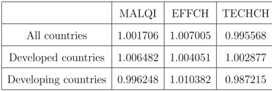
The application of the above methodology provides for each country, the Malmquist productivity index (MALM) and its components, efficiency change index (EFFCH) and technical change index (TECHCH) for each pairs of years in the sample. Then geometric averages of each index are computed for the en-tire 1970 − 1990 periods to show the average annual performance developments in productivity growth and its components for a particular country. For each index, a value greater than one indicates an average annual improvement in the performance of the country and a value less than one shows deterioration in per-formance. The mean MALM, EFFCH, TECHCH indices for all countries, and for developed and developing countries are reported in the table below:

MALQI EFFCH TECHCH

All countries 1.001706 1.007005 0.995568 Developed countries 1.006482 1.004051 1.002877 Developing countries 0.996248 1.010382 0.987215

Table 1 - Mean Malmquist Index and Its Decomposition

The mean Malmquist productivity index with a value slightly greater than one (1.001706) indicates that for all countries in the sample there has been produc-tivity gain on the average. Between the two groups of countries, there is a pro-ductivity gain in developed countries (0.06482% per year); there is a propro-ductivity loss in developing countries (0.03752% per year).

Developing countries have on average a higher efficiency change index, which indicates that this set of countries approach the ”best practice” frontier at a faster rate than high-income countries, and hence the catch-up process works in

(36)

the low-income countries. However, this set of countries are suffering from loss of productivity due to the other source of productivity growth-technical change (innovation)- which is in fact the main source of productivity growth for high-income countries (0.2877% technical change gain for developed countries and 1.2785% technical change loss for developing countries).

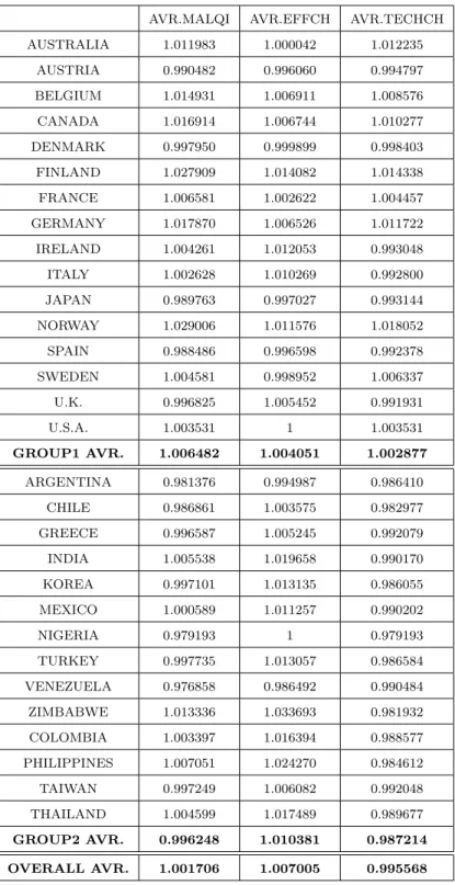
Average Malmquist indexes and their decompositions as efficiency change and technical change over the 1970 − 1990 periods can be seen below. Also averages among the groups of countries can be seen Table 2.

(37)

AVR.MALQI AVR.EFFCH AVR.TECHCH AUSTRALIA 1.011983 1.000042 1.012235 AUSTRIA 0.990482 0.996060 0.994797 BELGIUM 1.014931 1.006911 1.008576 CANADA 1.016914 1.006744 1.010277 DENMARK 0.997950 0.999899 0.998403 FINLAND 1.027909 1.014082 1.014338 FRANCE 1.006581 1.002622 1.004457 GERMANY 1.017870 1.006526 1.011722 IRELAND 1.004261 1.012053 0.993048 ITALY 1.002628 1.010269 0.992800 JAPAN 0.989763 0.997027 0.993144 NORWAY 1.029006 1.011576 1.018052 SPAIN 0.988486 0.996598 0.992378 SWEDEN 1.004581 0.998952 1.006337 U.K. 0.996825 1.005452 0.991931 U.S.A. 1.003531 1 1.003531 GROUP1 AVR. 1.006482 1.004051 1.002877 ARGENTINA 0.981376 0.994987 0.986410 CHILE 0.986861 1.003575 0.982977 GREECE 0.996587 1.005245 0.992079 INDIA 1.005538 1.019658 0.990170 KOREA 0.997101 1.013135 0.986055 MEXICO 1.000589 1.011257 0.990202 NIGERIA 0.979193 1 0.979193 TURKEY 0.997735 1.013057 0.986584 VENEZUELA 0.976858 0.986492 0.990484 ZIMBABWE 1.013336 1.033693 0.981932 COLOMBIA 1.003397 1.016394 0.988577 PHILIPPINES 1.007051 1.024270 0.984612 TAIWAN 0.997249 1.006082 0.992048 THAILAND 1.004599 1.017489 0.989677 GROUP2 AVR. 0.996248 1.010381 0.987214 OVERALL AVR. 1.001706 1.007005 0.995568 Table 2 - Malmquist Index and Its Decomposition for all countries

5.2 Estimations

As mentioned above, the purpose of the study is to find relationship between productivity measures and the groups of variables. This relationship can be

(38)

ex-pressed as:

Productivity measure_i = f (banking sector development indicators_i, economic condition indicatorsi,

financial sector variablesi,

institutional variablesi) (11)

In order to find the proper variables in the equation, first single variable es-timations are performed. Four different types of eses-timations varying according to the intercept and weighting (common intercept-no weighting, common inter-cept cross section weights, fixed effects-no weighting, fixed effects-cross section weights) are reported for all the regressions.

Given the regression model yit = αi+β0xit+²it, common intercept model takes

the individual effects, αi, same for all pool members. However, when fixed effects

model is used, αi is taken to be group specific constant term. (There is also

another approach, random effects approach, which treats intercepts as random variable across pool members. This approach is not included in the analysis.)

The different types of weighting styles used are no weighting and cross sec-tion weights models. In the no weighting model, all observasec-tions are given equal weight; on the other hand, in the cross section weights model, weights are esti-mated in the preliminary regression with equal weights and then are applied in weighted least squares in the second round.

5.3 Single Variable Estimations

In order to see which variables enter the regression significantly, first estima-tions are conducted with single explanatory variables in the following regression:

Productivity_it = β1i+ β2iExplanatory variable + ²it

The significance and signs of the four group of variables; banking sector de-velopment, economic conditions, financial sector development measures and

(39)

in-measured by the Malmquist indexes and their decompositions into technical effi-ciency and technological change indexes are used. For each explanatory variable four different regressions are estimated. These are common intercept and fixed effect models which either assumes the same intercept for all the countries in the sample or a different intercept for each country. These regressions are estimated again either with unweighted error variances or weighted error variances. Sections 7.1, 7.2 and 7.3 report the results for these single equation estimations. In the table only the probability values for the following hypothesis:

H0 : βi = 0

H1 : βi 6= 0

are reported for each explanatory variable. In evaluating the results, probability values less than 0.10 are considered to be significant (i.e. the probability of the coefficient being equal to zero is less than 0.10). Positive coefficients indicate a positive correlation between the dependent variable and the given variable; a negative sign for the coefficients indicate a negative correlation between the dependent variable and the variable.

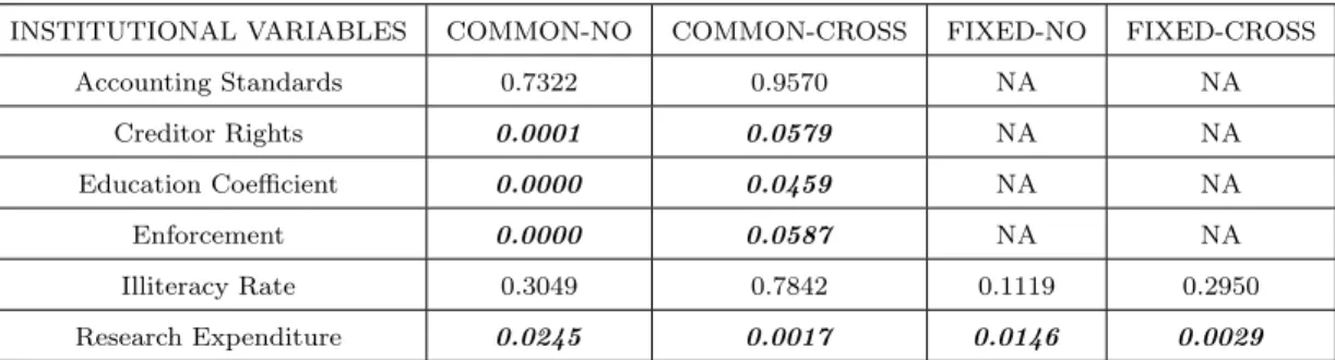
5.3.1 Malmquist Index Single Variable Estimation Results

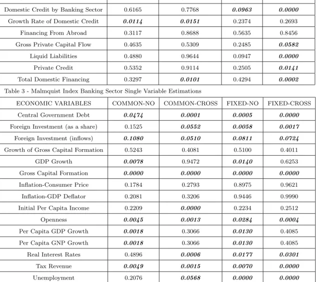
As can be seen from the Tables 3, 4, 5 and 6 (Section 7.1), domestic credit by banking sector, growth rate of domestic credit, total domestic financing and liquid liabilities have significant coefficients in two or more estimations types. Gross private capital flows, and credit to private sector have significant coefficients in one of the four different estimation types. Overall the size of the banking sector and especially the availability, liquidity and credit seem to have some determining power on the overall productivity of the countries.

Among the economic variables many of them have statistically significant co-efficients in single equation estimations. The variables that are significant in all estimation types are gross capital formation, foreign direct investment, openness and tax revenues. These are indicative of the fact that the accumulation of

(40)

cap-ital and the increase in the amount of capcap-ital stock increase the productivity of capital and labor use in the economies. The share of foreign direct investment, real interest rates and unemployment seem to have significant effects on the pro-ductivity changes. Other economic variables such as GDP growth rate and per capita GDP growth, and only in one regression initial per capita income, indicate that the convergence have some influence on productivity.

For the case of financial variables, the expected effect is not as direct as in the case of economic variables. Financial development measures will not also show the availability of liquidity for investment purposes in the economy like the banking sector variables does. But financial sector development measures are indicators of how well the market that transfer savings in the economy to loanable funds is working and hence the indirect measures of the opportunity of investment. Among the variables included into the single equation estimations, the number of listed companies and turn over ratio of the stocks traded are found significant in two of the regressions. Market capitalization measure and value of the stock traded have significant coefficients in one of the regressions estimated to explain the changes in the productivity.

In terms of the institutional measures, research turn out to have a strong significant effect on the productivity, with statistically significant coefficient in all four different regression estimations. Good accounting standards, the degree to which the legal system supports the creditors rights, efficiency in education, enforcement of the legal system and illiteracy turned out to have significant impact on the productivity levels in the economy.

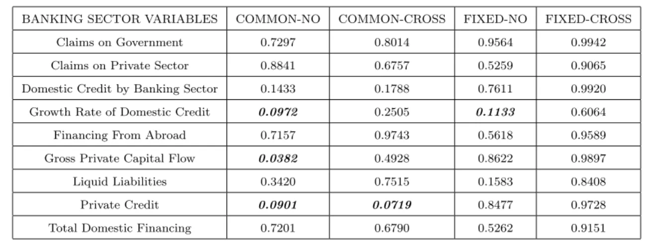
5.3.2 Efficiency Change Single Variable Estimation Results

When we perform the similar analysis for efficiency change, we find the results given in Tables 7, 8, 9 and 10 (Section 7.2). As can be seen from the table, among banking sector variables, growth rate of domestic credit and credit to private sector have significant coefficients in two estimation types. In addition to these,

(41)

estimation types.

Among the economic variables, gross capital formation, initial per capita in-come, openness, per capita GDP growth are significant in two estimation types. Moreover, GDP growth and tax revenue have significant coefficients in one of the estimation types.

When we consider the financial sector variables, we see that, similar to Malmquist index single variable estimation results, number of listed domestic companies, turnover ratio of stocks traded and total value of stocks traded enter the equation significantly.

For the case of institutional variables, all the variables (except research expen-diture) have significant coefficients. This suggests the importance of institutional regularization on the efficiency change of a country.

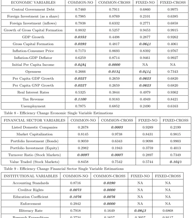
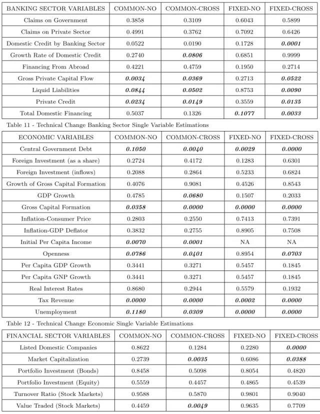
5.3.3 Technical Change Single Variable Estimation Results

Similar to Malmquist index and efficiency change, single variable estimations are performed for technical change. The results for technical change single variable estimation are given in Tables 11, 12, 13 and 14 (Section 7.3).

When we look at the banking sector variables, we see that gross private capital flow, liquid liabilities, credit to private sector and total domestic financing have significant coefficients in two or more estimation types.

Among the economic variables, central government debt, gross private capital formation, initial per capita income, openness, tax revenue and unemployment have significant coefficients in two or more estimation types. In addition to these, GDP growth enters the equation significantly in one of the four estimation types. In terms of financial sector variables, number of listed domestic companies, market capitalization and total value of stocks traded are significant in one or two estimation types. This suggests that these variables have an impact on the technical change.

Finally, for institutional variables, creditor rights, education coefficient, en-forcement and research expenditure have significant coefficients. Different from

(42)

efficiency change, research expenditure is significant in all four types of estimations and this suggests that research expenditure is a factor that boosts innovation.

5.4 Multi-Variable Estimations

After searching for the single variables which are significant in explaining the productivity indexes given, we tried to find the combination of these variables to explain the productivity indexes. In this case, regression equation looks like the following one:

Productivity_it = β1i+ β2iexplanatory variable + β3iexplanatory variable + . . .

. . . βkiexplanatory variable + ²it (12)

Very similar to the single variable estimations, the significance and signs of the four group of variables; banking sector development, economic conditions, fi-nancial sector development measures and institutional factors are examined and the productivity measured by the Malmquist index and its decompositions are used as dependent variables. For each explanatory variable four different regres-sions are estimated. These are common intercept and fixed effect models which either assumes the same intercept for all the countries in the sample or a differ-ent intercept for each country. These regression are estimated again either with unweighted error variances or weighted error variances. Sections 7.4, 7.5 and 7.6 report the results for these multi equation estimations. In the tables, only the probability values for the following hypothesis:

H0 : βi = 0

H1 : βi 6= 0

are reported for each explanatory variable. In evaluating the results, probability values less than 0.10 are considered to be significant (i.e. the probability of the coefficient being equal to zero is less than 0.10). Positive coefficients indicate

(43)

a negative sign for the coefficients indicate a negative correlation between the dependent variable and the variable.

5.4.1 Malmquist Index Multi Variable Estimation Results

As can be seen from the Tables 15, 16 and 17 (Section 7.4), many combinations of the variables are tested whether they are significant or not. First the double combinations of variables of the same group are tested. After getting the results of these combinations, complete equations that explain the Malmquist Index are searched for.

For the double variable estimations, domestic credit provided by banking sec-tor together with gross private capital flows, domestic credit provided by banking sector together with credit to private sector, domestic credit provided by bank-ing sector together with total domestic financbank-ing, domestic credit growth rate together with total domestic financing, gross private capital flows together with liquid liabilities, liquid liabilities together with total domestic financing, domestic credit growth rate together with claims on private sector are significant in explain-ing the Malmquist index as bankexplain-ing sector variables. Among economic variables, we tried the combinations of the variables which gave significant results in single estimations. When we look at the results in Table 16 (Section 7.4), we see that almost all of the combinations that we tried are significant in at least one type of estimations. That is, the combinations of central government debt, foreign direct investment, net inflow of foreign investment, GDP growth, openness, per capita GDP growth, real interest rate and tax revenue give significant results. In terms of financial sector variables, we see that number of listed domestic companies to-gether with market capitalization, number of listed domestic companies toto-gether with turnover ratio of stocks traded, number of listed domestic companies together with total value of stocks traded, number of listed domestic companies together with portfolio bond investment, number of listed domestic companies together with portfolio equity investment, market capitalization together with portfolio bond investment, market capitalization together with portfolio equity investment,

(44)

market capitalization together with total value of stocks traded, portfolio bond investment together with total value of stocks traded are significant in explaining the Malmquist index as financial sector variables.

After having the idea of possible significant variables, and after trying many combinations, we found two most significant equations given below:

1. ”MALM. INDEX = -0.0006dcredbybank + 0.0001openness - 0.0010realin-trate + 0.0008valuetraded”

where domestic credit by banking sector and real interest rate have the negative coefficients and openness and the total value of stocks traded have the positive coefficients. This first equation suggests that the openness and the total value of stocks traded positively effect the Malmquist index. On the other hand the real interest rate and domestic credit by banking sector has negative impact on the Malmquist index.

2. ”MALM. INDEX = 0.0005liquid + 0.0002openness - 0.0008realintrate + 0.0006valuetraded”

where liquid liabilities, openness and total value of stocks traded have pos-itive coefficients but real interest rate has a negative coefficient. This equa-tion suggests that liquid liabilities, openness and total value of stocks traded are positively correlated with Malmquist index, and real interest rate is neg-atively correlated with the Malmquist Index.

5.4.2 Efficiency Change Multi Variable Estimation Results

When we perform the similar analysis for efficiency change, we find the re-sults given in Tables 18, 19 and 20 (Section 7.5). As can be seen from the table, domestic credit by banking sector together with domestic credit growth rate are significant among banking sector variables in explaining the efficiency change. When economic variables are considered, we see that, GDP growth together with

(45)

growth, gross capital formation together with openness and openness together with per capita GDP growth have significant coefficients among economic vari-ables. For financial sector variables, number of listed domestic companies together with turnover ratio of stocks traded and portfolio equity investment together with total value of stocks traded are significant in explaining the efficiency change.

After observing these significant variables and trying many combinations, we found the following most significant equation:

”EFF. = 0.0003dcredbybank - 0.0005liquid - 0.0008infconsprice - 0.0001gro-capform + 0.0002lisdomcomp + 0.0004valuetraded”

In this equation, domestic credit by banking sector, number of listed domes-tic companies and total value of stocks traded have positive coefficients; liquid liabilities, inflation (consumer prices) and gross capital formation have negative coefficients. So, this regression equation explains that domestic credit by banking sector, number of listed domestic companies and total value of stocks traded are positively correlated with the efficiency component but liquid liabilities, inflation (consumer prices) and gross capital formation are negatively correlated with the efficiency component.

5.4.3 Technical Change Multi Variable Estimation Results

Similar to Malmquist index and efficiency change, multi variable estimations are performed for technical change. The results for technical change multi variable estimations are given in Tables 21, 22 and 23 (Section 7.6). As can be seen from the table, domestic credit by banking sector together with gross private capital flows, domestic credit by banking sector together with credit to private sector, do-mestic credit by banking sector together with total dodo-mestic financing, dodo-mestic credit by banking sector together with gross private capital flows, gross private capital flows together with liquid liabilities, gross private capital flows together with credit to private sector and credit to private sector together with total do-mestic financing have significant coefficients in explaining technology change in terms of banking sector variables. When we consider the economic variables, we

(46)

see that central government debt together with tax revenue, GDP growth together with gross capital formation, GDP growth together with real interest rate, GDP growth together with unemployment, gross capital formation together with real interest rate and gross capital formation together with unemployment are signif-icant in explaining the technology change. In terms of financial sector variables, number of listed domestic companies together with market capitalization, number of listed domestic companies together with portfolio equity investment, market capitalization together with portfolio bond investment, market capitalization to-gether with total value of stocks traded and portfolio equity investment toto-gether with total value of stocks traded have significant coefficients.

After having the idea of possible significant variables, and after trying many combinations, we found three most significant equations given below:

1. TECHNOLOGY = -0.0007liquid + 0.0010grocapform - 0.0005lisdomcomp where liquid liabilities and number of listed domestic companies are nega-tively, gross capital formation is positively correlated with the technology component.

2. TECHNOLOGY = 0.0005dcredbybank - 0.0003realintrate - 0.0008lisdom-comp

where real interest rate and number of listed domestic companies are nega-tively, domestic credit by banking sector is positively correlated with tech-nology component.

3. TECHNOLOGY = 0.0003dcredbybank + 0.0004unemployment + 0.0010turnover where all the components are positively correlated with the technology com-ponent.

When we examine the regression equations for technology component of the Malmquist index, we are unable to find as good equations as we did for Malmquist

(47)

for technology component, domestic credit by banking sector, liquid liabilities, unemployment, gross capital formation and number of listed domestic companies are the significant ones.

(48)

6 ESTIMATION OUTPUTS

6.1 Malmquist Index Single Variable Estimation

BANKING SECTOR VARIABLES COMMON-NO COMMON-CROSS FIXED-NO FIXED-CROSS Claims on Government 0.2484 0.4116 0.6506 0.8988 Claims on Private Sector 0.6189 0.5392 0.8033 0.9141 Domestic Credit by Banking Sector 0.6165 0.7768 0.0963 0.0000

Growth Rate of Domestic Credit 0.0114 0.0151 0.2374 0.2693 Financing From Abroad 0.3117 0.8688 0.5635 0.8456 Gross Private Capital Flow 0.4635 0.5309 0.2485 0.0582

Liquid Liabilities 0.4880 0.9644 0.0947 0.0000

Private Credit 0.5352 0.9114 0.2505 0.0141

Total Domestic Financing 0.3297 0.0101 0.4294 0.0002

Table 3 - Malmquist Index Banking Sector Single Variable Estimations

ECONOMIC VARIABLES COMMON-NO COMMON-CROSS FIXED-NO FIXED-CROSS Central Government Debt 0.0474 0.0001 0.0005 0.0000

Foreign Investment (as a share) 0.1525 0.0552 0.0058 0.0017

Foreign Investment (inflows) 0.1080 0.0510 0.0811 0.0724

Growth of Gross Capital Formation 0.5243 0.4081 0.5100 0.4011 GDP Growth 0.0078 0.9472 0.0140 0.6253 Gross Capital Formation 0.0000 0.0000 0.0000 0.0000

Inflation-Consumer Price 0.1784 0.2793 0.8975 0.9621 Inflation-GDP Deflator 0.2081 0.3206 0.9446 0.9990 Initial Per Capita Income 0.2209 0.0000 0.2234 0.2512 Openness 0.0045 0.0013 0.0284 0.0004

Per Capita GDP Growth 0.0018 0.3066 0.0130 0.4085 Per Capita GNP Growth 0.0018 0.3066 0.0130 0.4085 Real Interest Rates 0.4896 0.0006 0.0177 0.0301

Tax Revenue 0.0049 0.0015 0.0070 0.0000

Unemployment 0.2076 0.0568 0.0000 0.0000

Financial, economic, banking sector and institutional development and productivity