Relaxation-based viscosity mapping for magnetic particle imaging

(1)

PAPER

Relaxation-based viscosity mapping for magnetic

particle imaging

To cite this article: M Utkur et al 2017 Phys. Med. Biol. 62 3422

View the article online for updates and enhancements.

-Recent citations

A perspective on a rapid and radiation-free tracer imaging modality, magnetic particle imaging, with promise for clinical translation

Prashant Chandrasekharan et al

-Mathematical models for magnetic particle imaging

Tobias Kluth

-Implications of exposure to dextran-coated and uncoated iron oxide nanoparticles to developmental toxicity in zebrafish

Giovanna Medeiros Tavares de Oliveira et al

(2)

-Physics in Medicine & Biology

Relaxation-based viscosity mapping

for magnetic particle imaging

M Utkur1,2_{, Y Muslu}1,2_{and E U Saritas}1,2,3

1_{Department of Electrical and Electronics Engineering, Bilkent University, Ankara,}

Turkey

2_{National Magnetic Resonance Research Center (UMRAM), Bilkent University,}

Ankara, Turkey

3_{Neuroscience Graduate Program, Bilkent University, Ankara, Turkey}

E-mail: mustafa.utkur@bilkent.edu.tr

Received 29 July 2016, revised 2 October 2016 Accepted for publication 1 November 2016 Published 5 April 2017

Abstract

Magnetic particle imaging (MPI) has been shown to provide remarkable contrast for imaging applications such as angiography, stem cell tracking, and cancer imaging. Recently, there is growing interest in the functional imaging capabilities of MPI, where _{‘color MPI’ techniques have explored separating} different nanoparticles, which could potentially be used to distinguish nanoparticles in different states or environments. Viscosity mapping is a promising functional imaging application for MPI, as increased viscosity levels in vivo have been associated with numerous diseases such as hypertension, atherosclerosis, and cancer. In this work, we propose a viscosity mapping technique for MPI through the estimation of the relaxation time constant of the nanoparticles. Importantly, the proposed time constant estimation scheme does not require any prior information regarding the nanoparticles. We validate this method with extensive experiments in an in-house magnetic particle spectroscopy (MPS) setup at four different frequencies (between 250 Hz and 10.8 kHz) and at three different field strengths (between 5 mT and 15 mT) for viscosities ranging between 0.89 mPa _{· s–15.33 mPa · s. Our} results demonstrate the viscosity mapping ability of MPI in the biologically relevant viscosity range.

Keywords: magnetic particle imaging, viscosity mapping, relaxation, magnetic nanoparticles

(Some figures may appear in colour only in the online journal) M Utkur et al

Printed in the UK

3422

PHMBA7

Phys. Med. Biol.

PMB 10.1088/1361-6560/62/9/3422 Paper 9 3422 3439

Physics in Medicine _{& Biology}

Institute of Physics and Engineering in Medicine

2017

1361-6560

(3)

1. Introduction

Magnetic particle imaging (MPI) is a rapidly developing imaging modality (Gleich and Weizenecker 2005, Goodwill et al 2012, Saritas et al 2013a, Bauer et al 2015) with potential biomedical applications such as angiography (Weizenecker et al 2009, Lu et al 2013), stem cell tracking (Zheng et al 2015, 2016, Them et al 2016), cancer imaging (Yu et al 2016), guiding cardiovascular interventions (Haegele et al 2012), and predicting the effectiveness of magnetic hyperthermia (Murase et al 2015, Hensley et al 2016). MPI detects the response of superparamagnetic iron oxide (SPIO) nanoparticles to applied external magnetic fields, without any signal from the background tissue. This response is sensitive to the local environ-ment of the SPIOs such as the viscosity of the medium that they are in or their binding state to chemicals, showing a remarkable potential for functional imaging with MPI.

One potential functional imaging application for MPI is in vivo viscosity mapping. In liter-ature, blood viscosity was shown to change with hematocrit level (Pirofsky 1953), and several studies associated high hematocrit levels in the blood plasma with important diseases such as hypertension (Tibblin et al 1966), cerebral infarction (Tohgi et al 1978), angina pectoris (Burch and Depasquale 1965), ischemic heart disease (Fuchs et al 1984, 1990), and extensive coronary artery disease (Lowe et al 1980). High blood viscosity levels were also found to be prognostic of certain cancer types (Chandler and Schmer 1986, von Tempelhoff et al 2002). It was further suggested that cancer cells have increased cellular viscosity when compared to healthy cells (Guyer and Claus 1942). Importantly, for cell tracking applications, viscosity in a cell cytoplasm can give information regarding the uptake of external particles into the cell environment as well as activities occurring within the cell. Interactions in the cell environment such as signaling, transportation of molecules, enzymatic activity, binding effect were interre-lated with viscosity (Williams et al 1997, Rauwerdink and Weaver 2010a, 2011, Giustini et al

2012). Diagnoses of atherosclerosis (Deliconstantinos et al 1995), diabetes (Nadiv et al 1994), Alzheimer_{’s disease (Zubenko et al}1999), and neurological disorders (Fahey et al 1965) were found to be related with plasma fluidity, membrane viscosity, and serum viscosity. Given this extensive literature, measuring viscosity in vivo has important diagnostic and prognostic implications, making it a promising functional imaging application for MPI.

The relaxation behaviour of nanoparticles under zero-field (i.e. when an applied magnetic field is removed) is modeled by two different mechanisms: Neel relaxation where the magnetic moment of the nanoparticle aligns itself internally with the applied field, and Brownian relax-ation where the nanoparticle physically rotates to align its magnetic moment with the applied field. Extensive simulations showed the influence of particle parameters such as size and shape anisotropy, magnetization dynamics, and the sequence of applied fields (Weizenecker et al

2012, Graeser et al 2016). Theoretical modeling for Neel relaxation via Landau_{–Lifshitz–} Gilbert equation and for Brownian relaxation via Fokker_{–Planck equation were also presented} (Rogge et al 2013, Reeves and Weaver 2012). Due to the physical rotation of the nanoparticle, Brownian relaxation is directly influenced by the external environment, such as the viscosity of the medium. With this fact in mind, the monitoring of viscosity through the ratio of nano-particle magnetization harmonics was proposed, with potential extensions to system-matrix based MPI reconstruction (Rauwerdink and Weaver 2010b, Weaver and Kuehlert 2012). The relaxation induced signal delays in x-space based MPI reconstruction were also suggested as a possible tool for estimating the mobility of nanoparticles (Wawrzik et al 2013). Recent ‘color MPI’ studies have shown the capability of MPI to separate signals from different nano-particles (Rahmer et al 2015, Hensley et al 2015), which could in potential be applied to dif-ferentiate nanoparticles in different viscous environments. In these color MPI techniques, a successful separation relied on extensive calibration acquisitions that essentially characterize

(4)

the behaviour of the nanoparticles under different settings, or measurements at multiple drive field amplitudes to reveal the differences between the responses of nanoparticles. MPI cell tracking experiments have also shown that nanoparticles internalized into the cells displayed reduced resolution (Zheng et al 2015) or had altered signal characteristics when compared to nanoparticles in water (Them et al 2016), which could stem from viscosity effects on the relaxation behaviour of the nanoparticles. Hence, understanding the effects of viscosity on MPI signal is vital in developing the viscosity mapping capabilities of MPI for functional imaging purposes.

In this work, we propose a viscosity mapping technique for MPI that relies on the relaxa-tion induced changes in the nanoparticle response. We characterize these changes through an estimation of the relaxation time constant, without any a priori information on the nanoparti-cles. With extensive experiments in an in-house magnetic particle spectrometer (MPS) device, we show the drive field strength and frequency dependence of the relaxation time constant as a function of viscosity. The results provide guidance on MPI imaging parameters that can accentuate the signal differences between nanoparticles in environments with different vis-cosities. The proposed technique can be extended to imaging applications, facilitating the viscosity mapping potential of MPI.

2. Theory

In x-space MPI reconstruction, the ideal signal (also called the adiabatic signal) is denoted as (Goodwill and Conolly 2010);

s t B m x ˙ kGx kGx t˙ x x t s ideal 1 s ( )= ρ( ) [∗ ] _{( )} ( ) = L (2.1) where B1 (T A−1) is receiver coil sensitivity, m (Am2) is magnetic moment of the nanoparticle, ρ(x) (particles m−3_{) is density of nanoparticles along the x axis, k (m A}−1_{) is a nanoparticle} property, xs(t) is the time-dependent position of the field free point (FFP), and G is the

selec-tion field gradient strength (T m−1_u

0−1). In practice, the received MPI signal is affected by the relaxation behaviour of the SPIOs. Previous studies have modeled this effect as a temporal convolution of the ideal MPI signal with an exponential relaxation kernel (Croft et al 2012,

2016): s t( )=sideal( ) ( )t r t∗ (2.2) where, r t_{( )}1e t_{( )}u t τ = −τ (2.3) Here, τ is called the relaxation time constant and u(t) is the Heaviside step function. It has been verified via extensive experimental work that this phenomenological model accurately characterizes the MPI response for a wide range of frequencies and drive field amplitudes (Croft et al 2012, 2016).

In MPI, positive and negative half cycles of the drive field move the FFP forward and back across the scanned partial field-of-view (FOV), repetitively. As a result of this back and forth scanning process, the ideal MPI signal acquired during the positive and the negative scanning directions are _{‘mirror symmetric’, independent of the nanoparticle distribution ρ(x). Here,} mirror symmetry refers to the positive half cycle and the time-reversed and negated negative half cycle of the signal being identical. In the case of relaxation, however, the MPI signal is effectively _{‘blurred’ along the scanning direction, which in turn breaks the mirror symmetry}

(5)

between the two half cycles (Onuker and Saritas 2015, Muslu et al 2016). In theory, the relaxation time constant can be estimated from the half cycles of the MPI signal using the mir-ror symmetry of the underlying ideal MPI signal, without any a priori information about the nanoparticle type or distribution. The mathematical modeling behind this process is explained in detail in appendix A1. In this work, we apply this model to the nanoparticle signal from an MPS setup, with the goal of measuring the viscosity through estimating the relaxation time constant.

3. Materials and methods

3.1. Experimental setup

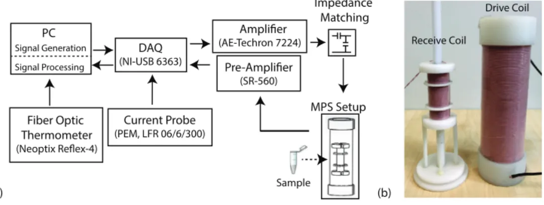
Figure 1 shows the overall experimental configuration. Our in-house magnetic particle spectro-meter (MPS) setup (also called an MPI relaxospectro-meter) had a drive coil that generates 0.97 mT A−1 magnetic field with 95% homogeneity in a 7 cm-long region down its bore (Utkur and Saritas

2015). The receive coil was a three-section gradiometer-type coil that allowed decoupling of the transmit and receive coils. This receive coil design had 7 layers of Litz wire, where each layer contained 41 turns in the middle and 21 turns on both sides. The measurement chamber inside the receive coil allowed a sample tube of 1.5 cm in length and 0.8 cm in diameter. According to our previous simulations, due to the symmetry in the design, an MPS setup that incorporates a three-section receive coil can utilize a shorter drive coil with 23% reduced power consumption to achieve results similar to a design that uses a two-section gradiometer-type receive coil (Utkur and Saritas 2015). The self-resonance of the receive coil was measured to be around 250 kHz. The drive field amplitude was calibrated via a Hall effect gaussmeter (LakeShore 475 DSP Gaussmeter) and monitored in real time via a Rogowski cur rent probe (LFR 06/6/300, Power Electronic Measurements Ltd).

The drive coil was impedance matched to an AC power amplifier (AE Techron 7224) using a capacitive network, which enabled maximum transfer to the load while low-pass filtering potential higher harmonics of the drive field. On the receive side, the nanoparticle signal was amplified with a low-noise voltage preamplifier (Stanford Research Systems SR560). The MPS setup was controlled with an in-house MATLAB script (Mathworks, Natick, MA). A data acquisition card (National Instruments, NI USB-6363) sent the drive field signal to be amplified to the power amplifier and digitized the signal from the receive chain. During the experiments, ambient temperature inside the measurement chamber was monitored using a fiber optic temperature probe (Neoptix Reflex-4).

3.2. Sample preparation and experimental procedures

Viscosity in the cell cytoplasm for an aqueous phase is reported to be around 1–2 mPa · s (close to the 0.89 mPa · s viscosity of pure water at 25 °C), and this number can become larger as the activity inside the cell increases (Kuimova et al 2009). Viscosity of the blood, on the other hand, is reported to be in the range of 1.3–7.8 mPa · s for hematocrit percentage in the total blood volume ranging between 14–76% (Pirofsky 1953). To provide biologically rel-evant results in light of this information, we prepared three different sets of samples:

3.2.1. Sample set #1. 11 samples with viscosities ranging between 0.89 mPa · s and 15.33 mPa · s were prepared. The total volume and nanoparticle amount in each sample was kept identical to avoid any Fe concentration bias in the results. Accordingly, each sample contained 50 µl of undiluted nanomag-MIP (Micromod GmbH, Germany) nanoparticles with 89 mmol

(6)

Fe/L concentration. These samples were then diluted to a total volume of 170 µl, with varying mixtures of deionized water and glycerol to reach the target viscosity levels at 25 °C (Sheely

1932). Here, 0.89 mPa · s corresponds to the viscosity of pure water, whereas 15.33 mPa · s corresponds to 68% glycerol by volume.

3.2.2. Sample set #2. To investigate the biological range in more detail, 20 samples with viscosity levels ranging from 0.89 mPa · s to 3.97 mPa · s were prepared following a procedure similar to the one described above. For this second set, the total sample volume was 200 µl, starting from an initial 80 µl volume of undiluted nanomag-MIP nanoparticles. Here, 3.97 mPa · s corresponds to the viscosity of 45% glycerol by volume.

3.2.3. Sample set #3. To compare the viscosity effect on different nanoparticles, 11 samples were prepared using VivoTrax ferucarbotran nanoparticles (Magnetic Insight Inc., USA) with 98 mmol Fe/L concentration. Note that this nanoparticle has the same chemical composition as Resovist. For this set, same viscosity levels (i.e. ranging from 0.89 mPa · s to 15.33 mPa · s) and volumes were used as in sample set #1.

Samples in set #1 were tested at four different drive field frequencies; 250 Hz, 550 Hz, 1.1 kHz, and 10.8 kHz, and under three different drive field peak amplitudes; 5 mT, 10 mT, and 15 mT. Samples in set #2 were tested at the same four frequencies, but only at 15 mT field amplitude. Samples in set #3 were tested at 550 Hz and 1.1 kHz, under two different drive field peak amplitudes: 10 mT and 15 mT. For each experiment, the amplified signal from the receive chain was digitized with 2 MS s−1_{bandwidth. Acquisition lengths} were chosen such that each cosine excitation pulse contained at least 35 periods. For each measurement, the mean of 16 acquisitions were recorded to increase signal-to-noise ratio (SNR). This step was performed first with no sample inside the measurement chamber to serve as the background measurement, and then with the sample. Overall, each experiment was repeated three times.

Figure 1. Overview of the experimental setup. (a) Arrows in the schematic denote the workflow of the transmit/receive chain for our in-house magnetic particle spectrometer (MPS) setup, which is controlled via a data acquisition card (DAQ) through MATLAB. A fiber optic thermometer and a current probe provide real-time monitoring of the temperature and the magnetic field in the MPS setup, respectively. (b) A picture of the receive coil and the drive coil. The receive coil is placed axially inside the drive coil and its vertical position is adjusted via the pedestal beneath, to minimize the mutual inductance between the two coils.

(7)

3.3. Data preprocessing

Acquired data sets were processed in MATLAB. For each experiment, the background signal was subtracted from the nanoparticle signal to remove the direct feedthrough and other potential interferences. An initial frequency selection was performed by choosing the higher harmonics of the drive field frequency in Fourier domain and setting all other frequencies to zero. This step removed the remaining direct feedthrough signal at the fundamental frequency, as well as the noise in non-harmonic frequencies that would oth-erwise reduce signal quality. A subsequent high-order zero-phase digital low-pass filter (LPF) was applied in time domain. The cut-off frequency of LPF was determined via com-paring the signal power at harmonic frequencies with the noise power at non-harmonic frequencies, which was computed before setting those frequencies to zero. Accordingly, the cut-off frequencies corresponded to 40th, 50th, 50th, and 18th harmonics for 250 Hz, 550 Hz, 1.1 kHz, and 10.8 kHz drive fields, respectively. The usage of fewer harmonics at 10.8 kHz was to avoid the self-resonance frequency of the receive coil, which contami-nated signals above 200 kHz.

3.4. Relaxation time constant estimation

The acquired signal contains both the relaxation effects, as well as a phase lag due to induc-tive/capacitive circuitry. Note that for the ideal MPI signal, the signal peaks would occur at central time points of half cycles, which would trivialize the phase lag estimation. In the case of relaxation, however, the signal peaks are inherently delayed in time with respect to the half-cycle centers.

Here, the relaxation time constant and the system delays were estimated simultaneously from the received signal, without any prior information. Accordingly, a sweep of phase lags, φ, between 0 and π were applied to the received signal and the signal was divided into positive/ negative half cycles for each phase lag case. The relaxation time constant, τ, was estimated from these half cycles as described in appendix A1. The signal was then Wiener deconvolved by the relaxation kernel r(t) given in (2.3). A necessary condition for the successful implemen-tation of the deconvolution step is to have sufficiently high SNR (Bente et al 2015), which was achieved via the data processing steps outlined in section 3.3. Next, the root-mean-squared error (RMSE) between the deconvolved positive half cycle, spos,ideal, and mirrored negative half cycle, sneg,ideal,mirr, was computed. This step was to check whether the mirror symmetry was restored after deconvolution. Finally, the {τ, φ} pair that minimized RMSE was chosen as the solution, i.e.

s t s t t , arg min d , pos,ideal neg,ideal,mirr 2 { } ( ) ( ) { }

∫

τ φ = − τ φ (3.1) The restoration of mirror symmetry via this technique was confirmed via visual inspection of results on randomly selected experimental data. The tails of the half cycles were excluded from the RMSE calculation step, as they corresponded to the lowest SNR regions of the sig-nal. Accordingly, 15% of the signal was cut from both sides of the half cycles during RMSE calculation. This choice is further explained in appendix A2.

Finally, as each experiment had three repetitions, the mean value and standard deviations across these repetitions were computed for each viscosity level at each drive field strength and frequency.

(8)

4. Results

Overall, 768 distinct experiments were performed. For sample set #1, nanomag-MIP nanoparticles at 11 viscosity levels were measured at 3 different field strengths, at 4 differ-ent frequencies, and with 3 repetitions (396 experimdiffer-ents). For sample set #2, nanomag-MIP nanoparticles at 20 viscosity levels were measured at a single field strength, at 4 different frequencies, and with 3 repetitions (240 experiments). For sample set #3, VivoTrax nanopar-ticles at 11 viscosity levels were measured at 2 different field strengths, at 2 different frequen-cies, and with 3 repetitions (132 experiments).

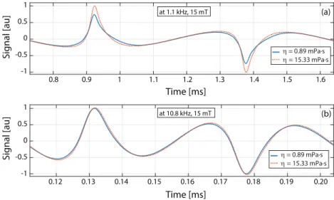
First, the effects of viscosity on the MPS signal were investigated at different drive field amplitudes and frequencies. Figure 2(a) compares two cases of MPS signals: at viscosity levels of 0.89 mPa _{· s (nanoparticles in water) and 15.33 mPa · s (nanoparticles in water/} glycerol mixture of 68% glycerol by volume), both acquired at 1.1 kHz and 15 mT drive field. Considering that both samples had the same iron content, one can note that the signal at low viscosity level is reduced when compared to that at high viscosity. In addition, the response at low viscosity is visibly wider, indicating an increased relaxation time constant. The estimated time constants were τ = 33 µs and τ = 24 µs for η = 0.89 mPa _{· s and η = 15.33 mPa · s,} respectively. Figure 2(b) compares the same samples at 10.8 kHz and 15 mT drive field. This time, in contrast to the results at 1.1 kHz, the signal at high viscosity is slightly wider than the one at low viscosity. The estimated times constants were τ = 3.5 µs and τ = 3.6 µs for η = 0.89 mPa _{· s and η = 15.33 mPa · s, respectively.}

The relaxation times constants were estimated for all MPS signals acquired. The results for sample set #1 (with 11 different viscosity levels) at four different drive field frequencies and three different drive field strengths are presented in figures 3 and 4. Error bars denote the mean estimated time constants and standard deviations over three repetition experiments. In

Figure 2. Effects of viscosity on nanoparticle signal. (a) The measured signal of nanomag-MIP nanoparticles at 1.1 kHz and 15 mT drive field are shown for low viscosity (0.89 mPa _{· s) and high viscosity (15.33 mPa · s) cases. The low viscosity} case displays a wider response with reduced peak amplitude. The calculated relaxation time constant for these two cases were τ = 33 µs and τ = 24 µs, respectively. (b) The

same samples were measured at 10.8 kHz and 15 mT drive field, yielding τ = 3.5 µs

and τ = 3.6 µs, respectively. Here, the high viscosity case has a slightly wider response

(9)

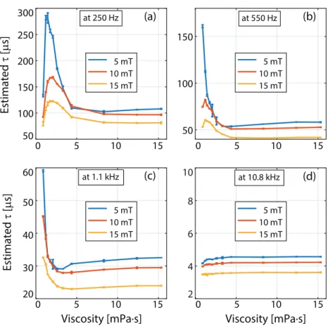
figure 3, for fixed frequency, estimated time constants decrease as field strength increases. The relaxation time constant as a function of viscosity displays a non-monotonic trend. Especially at low drive field frequencies and amplitudes (e.g. at 250 Hz and 5 mT), τ first increases sharply and then decreases with increasing viscosity, finally converging to a roughly constant value. At 10.8 kHz, on the other hand, τ slowly but steadily increases with increasing viscosity.

In figure 4, the same data are re-plotted, this time to highlight the effect of drive field fre-quency on estimated time constants. In figures 4(a)–(c), the time constants decrease with increasing frequency. Interestingly, one can see that there is a global trend in these curves, such that the same τ versus viscosity curve is scaled down and shifted towards the left as frequency increases. Figures 4(d)–(f) present these results with a normalized time axis, where the estimated time constants are normalized by the period of the drive field at each frequency, and multiplied by 100. Effectively, this unified y-axis gives an indication of the percentage effect of relaxation delays at each frequency. Overall, for fixed drive field amplitude, the relaxation effects are more prominent at higher frequencies. Exceptions to this trend are low viscosity and low drive field strengths, where the trends can be reversed (e.g. at 5 mT for viscosities lower than 3 mPa · s).

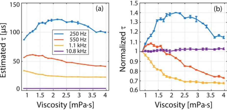
To investigate the biologically more relevant viscosities of up to 4 mPa · s, the time con-stants for sample set #2 with 20 different viscosity levels between 0.89 mPa · s and 4 mPa · s were estimated at four different drive field frequencies with 15 mT field strength. Another

Figure 3. Relaxation time constants as a function of viscosity, at four different drive field frequencies for sample set #1 (nanomag-MIP at 11 different viscosities ranging between 0.89 mPa _{· s to 15.33 mPa · s). Error bars denote the mean values and standard} deviations over three repetition experiments.

(10)

motivation for this second set of experiments was to ensure that the τ versus viscosity curves did not exhibit erratic jumps with a slight variation in viscosity. The results given in figure 5(a) are consistent with the low viscosity portions of the results in figure 4(c), as no erratic behav-iour is observed. Note that the estimated time constants at 2.5 mPa · s and 3.6 mPa · s showed slight deviations from the overall trends. These deviations could stem from pipetting errors during the mixing of water and glycerol, as a small variation in glycerol percentage can sig-nificantly alter the viscosity level of the mixture. In figure 5(b), the relaxation time constants are normalized by that of nanoparticles in water (i.e. the lowest viscosity of 0.89 mPa · s), so that the percentage change in τ can be visualized. At 250 Hz, τ first increases by 40% at around 2.2 mPa · s, then gradually decreases. At 1.1 kHz, τ monotonically decreases, showing a 32% reduction at around 4 mPa · s. At 10.8 kHz, on the other hand, τ increases by only 2% within this viscosity range.

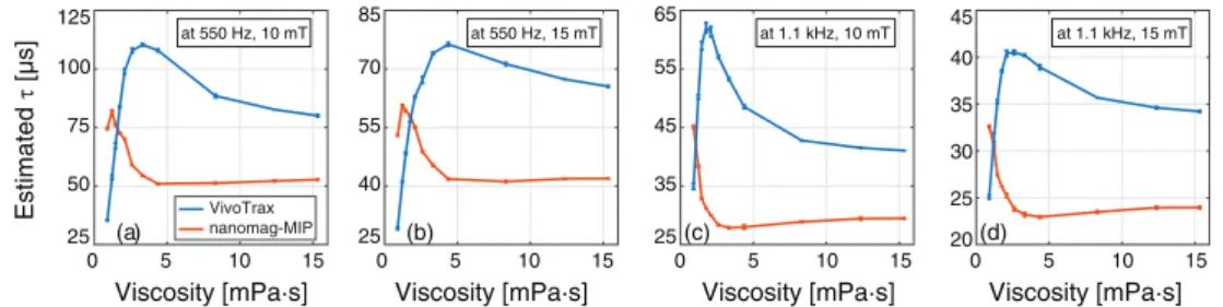
To provide a better understanding of the effects of viscosity on different nanoparticles, experiments were performed with VivoTrax nanoparticles at 11 different viscosity levels (sample set #3). The results are given in figure 6, in comparison with nanomag-MIP nano-particles under the same drive field conditions. Accordingly, the estimated time constants for VivoTrax are larger than those for nanomag-MIP, in general. Importantly, the relaxation time constants for VivoTrax display a non-monotonic trend as a function of viscosity, as was the case for nanomag-MIP. Furthermore, the global trend seen in nanomag-MIP is also observed for VivoTrax: the same τ versus viscosity curve is scaled down and shifted towards the left with increasing frequency, as can be seen comparing figures 6(a) with (c).

Figure 4. Relaxation time constants as a function of viscosity, at three different drive field strengths for sample set #1 (nanomag-MIP at 11 different viscosities ranging between 0.89 mPa _{· s–15.33 mPa · s). Error bars denote the mean values and standard} deviations over three repetition experiments. (a)_{–(c) The same data as in figure}3, re-plotted to emphasize the effect of drive field frequency at a fixed field strength. (d)_–(f) The results in a unified y-axis, where the estimated time constants are normalized by the period of the drive field at each frequency, multiplied by 100.

(11)

During all experiments, the ambient temperature inside the measurement chamber remained between 23–36 °C, which corresponds to a minor 4% variation in absolute temperature in Kelvins. This variation was due to resistive heating of the drive coil under currents reaching 22 A, which causes a power dissipation of about 350 W. Nonetheless, during signal acquisi-tion, each sample tube stayed in the measurement chamber for only 5 s at a time. In a separate control experiment, we also measured the temperature inside the sample tubes for the case when the chamber temperature was at 36 °C. Accordingly, during the 5 s interval that the sample was exposed to convective heat transfer, its temperature only changed by 0.3–0.4 °C. Hence, we do not expect any temperature bias for the results reported in this work.

5. Discussion

Viscosity sensing is currently infeasible with ultrasound, magnetic resonance imaging, or other preclinical imaging techniques. This work demonstrated the potential of MPI for viscos-ity mapping through the estimation of the nanoparticle relaxation time constant. As shown in the results in figures 3_–5, the trend in the τ versus viscosity curves strongly depend on the drive field strength and frequency. Ideally, a quantitative viscosity mapping technique should provide a one-to-one mapping of the measured parameter to the viscosity level. Such a tech-nique should also show a sufficiently large variation of the measured parameter as a function of viscosity, such that the viscosity can be determined accurately. For the biologically relevant range investigated in figure 5, these requirements are best satisfied by the measurements at 1.1 kHz, where the relaxation time constant monotonically decreases with increasing viscos-ity and displays greater than 30% variation. At 10.8 kHz, on the other hand, the time constant remains almost constant at different viscosity levels. These findings imply that the regular MPI operating frequencies of 25 kHz or 150 kHz are not optimal for viscosity mapping pur-poses. For the very low drive field frequencies around 250 Hz, on the other hand, τ is a non-monotonic function of viscosity, which would create an ambiguity in viscosity mapping. A potential solution at those frequencies could be to perform measurements at two different field strengths to determine the viscosity level.

Figure 5. Relaxation time constant versus viscosity for the biologically more relevant range of viscosities, for sample set #2 (nanomag-MIP at 20 different viscosities ranging between 0.89 mPa _{· s–3.97 mPa · s), measured at four different frequencies} at 15 mT field strength. Error bars denote the mean values and standard deviations over three repetition experiments. (a) Estimated time constants and (b) time constants normalized by that of nanoparticles in water to highlight the percentage change in τ

(12)

The well-known Brownian relaxation time constant of nanoparticles is given as τ = 3Vη/kBT, where the time constant increases linearly with viscosity, which is clearly not the case for the results shown in this work. It should be emphasized that the Neel and Brownian time constants are valid for the zero field case only, i.e. when an applied external magnetic field is suddenly removed. Hence, they do not model the more complex cases such as a sinusoi-dal external field. For those cases, simulation results solving Landau–Lifshitz–Gilbert equa-tion or Fokker–Planck equation were presented (Reeves and Weaver 2012, Rogge et al 2013). A previous method considered a dynamic magnetization model, where the ratio of 5th to 3rd harmonics of nanoparticle magnetization was utilized to probe viscosity. Accordingly, a non-monotonic trend was observed as a function of viscosity, both in simulations as well as in experiments with Feridex in various gelatin concentrations (Rauwerdink and Weaver 2010b). Here, the relaxation time constant in (2.2) and (2.3) is a lumped parameter that models the blurring effect in the time-domain MPI signal, without considering the underlying physical mechanisms. Still, the result in figure 2(a) that displays a visibly narrower response at higher viscosity level is counter intuitive, as one would expect a slower nanoparticle response with increasing viscosity. This could potentially be due to the chemical differences between the water solution versus the high viscosity water/glycerol mixture, which can potentially affect the interaction of the nanoparticles with each other and with the medium. Experiments in solutions with similar viscosities but with different chemical properties could help in under-standing this effect.

Previous studies have demonstrated that the MPI signal properties strongly depend on the nanoparticle type (Ferguson et al 2015). The experiments here were performed using nanomag-MIP and VivoTrax, where both nanoparticles displayed similar non-monotonic trends. Interestingly, the response of VivoTrax at 1.1 kHz and 10 mT was very similar to the response of nanomag-MIP at 550 Hz and 15 mT, as can be seen in figure 6. These similarities imply that the same physical mechanism is taking place for both nanoparticles, albeit at differ-ent strengths. It should be noted that both of these nanoparticles are multi-core nanoparticles with clusters made up of smaller nanoparticles (Eberbeck et al 2013). It remains to be shown whether similar trends are valid for single-core nanoparticles with large diameters.

One important factor to take into account during viscosity mapping with the proposed tech-nique is the homogeneity of the drive field. As seen in figure 3, for a fixed frequency, changes in drive field amplitude significantly change the estimated relaxation time constant. Hence, to ensure a quantitative mapping of the viscosity during 3D imaging applications, either the drive field needs to be highly homogeneous within the field-of-view (FOV), or one needs to

25 40 55 70 85 at 550 Hz, 15 mT Viscosity [mPa·s] (b) 25 50 75 100 125 Viscosity [mPa·s] at 550 Hz, 10 mT 0 5 10 15 0 5 10 15 0 5 10 15 0 5 10 15 nanomag-MIP VivoTrax (a) 25 35 45 55 65 at 1.1 kHz, 10 mT Viscosity [mPa·s] (c) ₂₀ 25 30 35 40 45 at 1.1 kHz, 15 mT Viscosity [mPa·s] (d) Estimated t [µs]

Figure 6. Effects of viscosity on the relaxation time constants of two different nanoparticles. VivoTrax and nanomag-MIP nanoparticles were measured at four different drive field conditions, and at 11 different viscosities ranging between 0.89 mPa _{· s–15.33 mPa · s. Error bars denote the mean values and standard deviations over} three repetition experiments.

(13)

know the field map within the FOV. Another important consideration is the human safety limits of the applied drive fields (Saritas et al 2013b, 2015, Schmale et al 2013). According to the results shown in this work, frequencies around 1 kHz have the potential to provide a one-to-one viscosity mapping capability. For 1 kHz, the magnetostimulation safety limit in the human torso can roughly be estimated as 20 mT-peak (Saritas et al 2013b). Hence, the results presented at 1.1 kHz and 15 mT-peak field strength are actually applicable according to the human safety limits of MPI. It should be noted that operating at a lower frequency than the current MPI frequencies (25 kHz, or lately 150 kHz) would have both advantages and disad-vantages in terms of image quality. Previous work has shown that peak signal values changed approximately linearly with the drive field frequency and amplitude (Weber et al 2015, Croft et al2016). Similarly, in our experiments, the received signal strength (before the low-noise preamplifier) at 1.1 kHz was around 10 times lower than that at 10.8 kHz for the same drive field amplitude (results not shown). Hence, the image SNR would decrease when operating at lower frequencies. On the other hand, lower drive field frequencies could yield better resolu-tion images, as previously demonstrated via resoluresolu-tion measurements in a relaxometer setup (Croft et al 2016). Likewise in our experiments, the nanoparticle signal at 1.1 kHz had a nar-rower peak than that at 10.8 kHz for the same drive field amplitude, as seen in figure 2.

The exponential model in (2.2) and (2.3) was first proposed and validated for frequencies between 4.4 kHz and 25 kHz (Croft et al 2012, 2016). One assumption inherent in this model is that the ideal nanoparticle response without relaxation effects is symmetric with respect to applied field (i.e. the signal peaks occur at central time points of half cycles), which may not be the case for nanoparticles with shape anisotropy or for ferromagnetic nanoparticles. Even in those cases, however, the proposed method could potentially detect the _{‘relative’ changes in} delay caused by lower/higher viscosity environments. For the multi-core nanoparticles tested here, our analysis shows that the exponential model provides a good fit to the experimental data at 1.1 kHz and 10.8 kHz. At lower drive field frequencies, however, we see that the relaxa-tion deconvolved signal does not fully revert to a mirror symmetric signal. In appendix A2, we analyzed the effect of truncating the tails of the half cycles during τ estimation. In theory, if the model worked perfectly, it should yield identical τ independent of truncation percent-age. This, however, is not the case at low drive field amplitudes and frequencies. These results indicate that the exponential model provides a better fit to the measured signal at frequencies in the kHz range.

At all frequencies tested in this work, the relaxation time constants showed an asymptotic convergence for viscosity levels above 5 mPa _{· s, remaining almost flat above 8 mPa · s. These} results indicate that viscosity mapping with this technique may not be feasible at very high viscosity levels. However, there is good evidence in the literature that viscosities below 5 mPa · s are biologically more relevant. For example, it has been previously reported that hemato-crit level exceeding 46% (>2.8 mPa _{· s) is considered as an important risk factor for cerebral} infarction, atherosclerosis in the arteries, and hypertension (Tohgi et al 1978). In another study, elevated viscosity levels from 1.48 mPa _{· s to 1.71 mPa · s due to myocardial infarction} was reported (Fuchs et al 1990). These viscosity levels are within the mapping capabilities of the proposed technique, demonstrating the potential of MPI imaging to provide critical functional information.

6. Conclusion

In this work, we have demonstrated the viscosity mapping capability of MPI through proof-of-concept experiments in an MPS device. The proposed technique takes advantage of the

(14)

underlying mirror symmetry in the time-domain MPI signal to blindly estimate a relaxation time constant. The experimental results at various drive field frequencies suggest that a rela-tively low drive field frequency of around 1 kHz is promising for a one-to-one viscosity map-ping. Future imaging applications exploiting the MPI signal_{’s dependence on local viscosity} of the nanoparticles will benefit from the results provided in this work.

Acknowledgments

The authors would like to thank Akbar Alipour for his assistance in the experimental proce-dures, and to Tarik Reyhan for valuable discussions. This work was supported by the Scien-tific and Technological Research Council of Turkey through TUBITAK Grants (114E167), by ERA.Net RUS PLUS Program (TUBITAK 215E198), by the European Commission through FP7 Marie Curie Career Integration Grant (PCIG13-GA-2013-618834), by the Turkish Acad-emy of Sciences through TUBA-GEBIP 2015 program, and by the BAGEP Award of the Science Academy.

Appendix

A1. Relaxation time constant estimation

A sinusoidal drive field superimposed to a piecewise constant focus field results in a so called ‘linear’ MPI trajectory, which scans a partial field-of-view (FOV) back and forth, repeatedly. With this trajectory, the ideal MPI signal (i.e. the signal without relaxation effects) demon-strates what can be called a ‘mirror symmetry’ between signal parts acquired during the posi-tive and the negaposi-tive scanning directions. Accordingly, these ideal half-cycle signals can be expressed as follows:

spos, ideal( )t = −sneg,ideal( )− =t shalf( )t

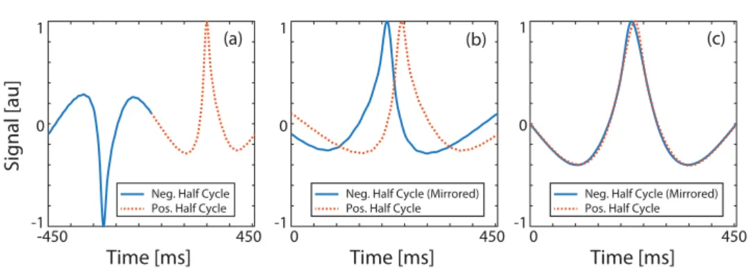
(A.1) Here, _{‘mirroring’ is defined as time reversal and negation of a signal. Previously, MPI signal} with relaxation has been modeled as a convolution of nanoparticles_{’ Langevin response with a} relaxation kernel, as given in (2.2) and (2.3). In principle, the relaxation process blurs the sig-nal along the scanning direction, breaking the mirror symmetry between the two half cycles. To demonstrate this point, figures A1(a) and (b) display the lost mirror symmetry for a mea-sured MPS signal acquired at 1.1 kHz and 15 mT drive field for nanomag-MIP nanoparticles. In theory, the half cycles shown in figure A1(b) would overlap exactly if the nanoparticles did not exhibit any relaxation behaviour.

Using the convolution-based formulation for the MPI signal, the half cycles in the case of relaxation can be expressed as:

spos( )t =spos,ideal( ) ( )t r t∗ =shalf( ) ( )t r t∗

(A.2) sneg( )t =sneg,ideal( ) ( )t r t∗ = −shalf( ) ( )− ∗t r t

(A.3) Note that shalf(t) is the ideal half-cycle signal. Using the exponential model for r(t), these two equations can be solved simultaneously to reveal both τ and shalf(t) (Onuker and Saritas 2015,

(15)

Muslu et al 2016). Here, we are particularly interested in the relaxation time constant τ, which can be expressed in closed form in the Fourier domain:

r t R f f 1 1 i2 { ( )}= ( )= ₍ _{π τ}₎ + F (A.4)

{

( )

}

= ( )= ( ) ( )⋅

F spost Spos f Shalf f R f

(A.5)

{

( )

}

= ( )= − ( ) ( )− ⋅

F snegt Sneg f Shalf f R f

(A.6) Here, (A.4) is the known 1D Fourier transform of an exponential function and (A.6) fol-lows from time reversal property of Fourier transform. Since shalf(t) is real valued, its Fourier transform Shalf( f ) has conjugate symmetry property. Accordingly, the last equation can be re-written as

{

( )

}

= ( )= − ∗ ( ) ( )⋅

F snegt Sneg f Shalf f R f

(A.7) where the superscript star sign denotes the conjugation operation. Finally, combining (A.4)_–(A.7), we can express the relaxation time constant as follows:

(

( ) ( ) ( )( )

)

τ π = + − ∗ ∗ S f S f f S f S f i2 pos neg pos neg (A.8) Once this time constant is estimated, the signal can be deconvolved by the relaxation kernel, r(t), to reveal the underlying ideal MPI signal. In theory, this deconvolution step recovers the mirror symmetry between the half cycles. This process is demonstrated in figure A1(c).

In this work, the relaxation time constant and system delays were estimated simultaneously (see section 3.4). The {τ, φ} pair that minimized the RMSE between the deconvolved versions of the positive and the mirrored negative half cycles was chosen as the solution.

Figure A1. Estimating the relaxation time constant directly from the measured MPS signal. (a) Measured MPS signal for nanomag-MIP nanoparticles at 1.1 kHz and 15 mT drive field, for the case of a low viscosity solution (approximately 1.22 mPa _{· s). The} relaxation effect on the signal is clearly visible. (b) The positive half cycle and the mirrored (i.e. time reversed and negated) negative half cycle are overlaid. If the signal had not contained any relaxation effects, these two half cycles would overlap exactly. Due to relaxation, however, each half cycle is _{‘blurred’ along the scanning direction.} The time constant estimation scheme described in appendix A1 yields τ = 32.9 µs.

(c) The measured signal can then be deconvolved by the relaxation kernel with the estimated time constant, which reveals the underlying mirror symmetry.

(16)

A2. Influence of tail truncation on estimated time constants

The model in (2.2) and (2.3) is phenomenological, i.e. it is based on extensive experimental work that demonstrates a good fit to this model (Croft et al 2012). If this model could mimic the relaxation behaviour perfectly, deconvolution with the correct relaxation kernel would restore mirror symmetry completely. As shown in figure A1(c), the half cycles after deconvo-lution display close to perfect mirror symmetry, notwithstanding a small region of mismatch at the signal peak locations. The mismatch in the peaks could be avoided by assigning more weight to the goodness-of-fit at the center of half cycles. Doing so, however, would worsen the overlap in the remaining portions of the half cycles.

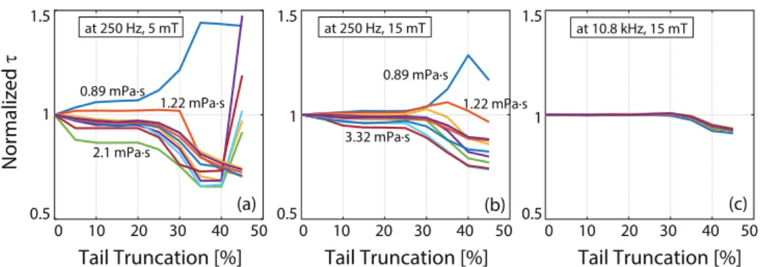
We have analyzed the influence of truncating different percentages of the deconvolved half-cycle tails during RMSE calculations. For example, when 100% of the half cycles are utilized (i.e. 0% truncation), the RMSE calculation takes into account the overlap of both the tails and the center of the half cycle. Alternatively, one can truncate a percentage of the tails before calculating the RMSE, such that the overlap of the central regions becomes the main target. Figure A2 shows the effect of tail truncation percentage on the estimated relaxation time constants. The values are normalized to show the overall trends. Here, a 10% truncation indicates 10% of half cycles truncated from both tails, with the remain-ing central 80% utilized in RMSE calculation. If the relaxation model worked perfectly, one would expect to see a flat τ versus truncation percent curve, i.e. estimated τ would be independent of the truncation percentage. This is in fact the case at high frequency and high field amplitude, as seen in figure A2(c). At low frequencies and low field amplitudes, however, a large truncation percentage yields diverging results. These results indicate that the exponential model is a better fit at high drive field frequencies and amplitudes. In all cases considered in this work, τ estimation remained flat for truncation percentages ranging between 10% and 20%. Accordingly, a truncation percentage of 15% was utilized in all τ estimations presented in this work.

Figure A2. Influence of tail truncation on the estimated relaxation time constants. If the relaxation model worked perfectly, these curves would be horizontally flat, yielding constant τ estimation independent of truncation percentage. At low drive field amplitude

and frequency as in (a), large truncation percentage yields diverging results, whereas zero truncation shows a slight variation from the expected flat response. In contrast, at high drive field amplitude and frequency as in (c), the estimations remain constant up to 35% tail truncation. In all cases, tail truncations between 10%_{–20% yielded constant τ} estimations. Results are for nanomag-MIP nanoparticles.

(17)

References

Bauer L M, Situ S F, Griswold M A and Samia A C S 2015 Magnetic particle imaging tracers: state-of-the-art and future directions J. Phys. Chem. Lett. 6 2509–17

Bente K, Weber M, Graeser M, Sattel T F, Erbe M and Buzug T M 2015 Electronic field free line rotation and relaxation deconvolution in magnetic particle imaging IEEE Trans. Med. Imaging 34 644–51

Burch G E and Depasquale N P 1965 Hematocrit, viscosity and coronary blood flow supported by grants from the US Public Health Service Dis. Chest 48 225–32

Chandler W L and Schmer G 1986 Evaluation of a new dynamic viscometer for measuring the viscosity of whole blood and plasma Clin. Chem. 32 505–7

Croft L R, Goodwill P W and Conolly S M 2012 Relaxation in x-space magnetic particle imaging IEEE

Trans. Med. Imaging31 2335–42

Croft L R, Goodwill P W, Konkle J J, Arami H, Price D A, Li A X, Saritas E U and Conolly S M 2016 Low drive field amplitude for improved image resolution in magnetic particle imaging Med. Phys.

43 424–35

Deliconstantinos G, Villiotou V and Stavrides J 1995 Modulation of particulate nitric-oxide synthase activity and peroxynitrite synthesis in cholesterol-enriched endothelial-cell membranes Biochem.

Pharmacol.49 1589–600

Eberbeck D, Dennis C L, Huls N F, Krycka K L, Gruttner C and Westphal F 2013 Multicore magnetic nanoparticles for magnetic particle imaging IEEE Trans. Magn. 49 269–74

Fahey J L, Barth W F and Solomon A 1965 Serum hyperviscosity syndrome JAMA 192 464–7

Ferguson R M et al 2015 Magnetic particle imaging with tailored iron oxide nanoparticle tracers IEEE

Trans. Med. Imaging34 1077–84

Fuchs J, Pinhas A, Davidson E, Rotenberg Z, Agmon J and Weinberger I 1990 Plasma viscosity, fibrinogen and haematocrit in the course of unstable angina Eur. Heart J. 11 1029–32

Fuchs J, Weinberger I, Rotenberg Z, Erdberg A, Davidson E, Joshua H and Agmon J 1984 Plasma viscosity in ischemic heart disease Am. Heart J. 108 435–9

Giustini A J, Perreard I, Rauwerdink A M, Hoopes P J and Weaver J B 2012 Noninvasive assessment of magnetic nanoparticle-cancer cell interactions Integr. Biol. 4 1283_–8

Gleich B and Weizenecker J 2005 Tomographic imaging using the nonlinear response of magnetic particles Nature 435 1214_–7

Goodwill P W and Conolly S M 2010 The x-space formulation of the magnetic particle imaging process: 1D signal, resolution, bandwidth IEEE Trans. Med. Imaging 29 1851_–9

Goodwill P W, Saritas E U, Croft L R, Kim T N, Krishnan K M, Schaffer D V and Conolly S M 2012

x-space MPI: magnetic nanoparticles for safe medical imaging Adv. Mater. 24 3870_–7

Graeser M, Bente K, Neumann A and Buzug T M 2016 Trajectory dependent particle response for anisotropic mono domain particles in magnetic particle imaging J. Phys. D: Appl. Phys.

49 45007

Guyer M F and Claus P E 1942 Increased viscosity of cells of induced tumors Cancer Res. 2 16_–8 Haegele J, Rahmer J, Gleich B, Borgert J, Wojtczyk H, Panagiotopoulos N, Buzug T M, Barkhausen J

and Vogt F M 2012 Magnetic particle imaging: visualization of instruments for cardiovascular intervention Radiology 265 933_–8

Hensley D, Goodwill P, Croft L and Conolly S 2015 Preliminary experimental x-space color MPI 2015

5th Int. Workshop on Magnetic Particle Imaging (IWMPI) (Istanbul) p 1

Hensley D, Goodwill P, Dhavalikar R, Tay Z W, Zheng B, Rinaldi C and Conolly S M 2016 Imaging and localized nanoparticle heating with MPI 6th Int. Workshop on Magnetic Particle Imaging (IWMPI)

(Lübeck) p 171

Kuimova M K, Botchway S W, Parker A W, Balaz M, Collins H A, Anderson H L, Suhling K and Ogilby P R 2009 Imaging intracellular viscosity of a single cell during photoinduced cell death

Nat. Chem.1 69_–73

Lowe G D, Drummond M M, Lorimer A R, Hutton I, Forbes C D, Prentice C R and Barbenel J C 1980 Relation between extent of coronary artery disease and blood viscosity BMJ 280 673_–4

Lu K, Goodwill P W, Saritas E U, Zheng B and Conolly S M 2013 Linearity and shift invariance for quantitative magnetic particle imaging IEEE Trans. Med. Imaging 32 1565_–75

Murase K, Aoki M, Banura N, Nishimoto K, Mimura A, Kubayabu T and Yabata I 2015 Usefulness of magnetic particle imaging for predicting the therapeutic effect of magnetic hyperthermia

(18)

Muslu Y, Utkur M and Saritas E U 2016 Calibration-free color MPI 6th Int. Workshop on Magnetic

Particle Imaging (IWMPI) (Lübeck) p 10

Nadiv O, Shinitzky M, Manu H, Hecht D, Roberts C T, LeRoith D and Zick Y 1994 Elevated protein tyrosine phosphatase activity and increased membrane viscosity are associated with impaired activation of the insulin receptor kinase in old rats Biochem. J. 298 443_–50

Onuker G and Saritas E U 2015 Simultaneous relaxation estimation and image reconstruction in MPI 5th

Int. Workshop on Magnetic Particle Imaging (IWMPI) (Istanbul) p 1

Pirofsky B 1953 The determination of blood viscosity in man by a method based on Poiseuille_{’s law}

J. Clin. Invest.32 292_–8

Rahmer J, Halkola a, Gleich B, Schmale I and Borgert J 2015 First experimental evidence of the feasibility of multi-color magnetic particle imaging Phys. Med. Biol. 60 1775_–91

Rauwerdink A M and Weaver J B 2011 Concurrent quantification of multiple nanoparticle bound states

Med. Phys.38 1136_–40

Rauwerdink A M and Weaver J B 2010a Measurement of molecular binding using the Brownian motion of magnetic nanoparticle probes Appl. Phys. Lett. 96 033702

Rauwerdink A M and Weaver J B 2010b Viscous effects on nanoparticle magnetization harmonics

J. Magn. Magn. Mater.322 609_–13

Reeves D B and Weaver J B 2012 Simulations of magnetic nanoparticle Brownian motion J. Appl. Phys.

112 124311

Rogge H, Erbe M, Buzug T M and Ludtke-Buzug K 2013 Simulation of the magnetization dynamics of diluted ferrofluids in medical applications Biomed. Tech. 58 601_–9

Saritas E U, Goodwill P W and Conolly S M 2015 Effects of pulse duration on magnetostimulation thresholds Med. Phys. 42 3005_–12

Saritas E U, Goodwill P W, Croft L R, Konkle J J, Lu K, Zheng B and Conolly S M 2013a Magnetic particle imaging (MPI) for NMR and MRI researchers J. Magn. Reson. 229 116_–26

Saritas E U, Goodwill P W, Zhang G Z and Conolly S M 2013b Magnetostimulation limits in magnetic particle imaging IEEE Trans. Med. Imaging 32 1600_–10

Schmale I, Gleich B, Schmidt J, Rahmer J, Bontus C, Eckart R, David B, Heinrich M, Mende O, Woywode O, Jokram J and Borgert J 2013 Human PNS and SAR study in the frequency range from 24 to 162 kHz 2013 5th Int. Workshop on Magnetic Particle Imaging (IWMPI) (Berkeley) p 1

Sheely M L 1932 Glycerol viscosity tables_{—industrial & engineering chemistry (ACS Publications) Ind.}

Eng. Chem.24 1060_–4

Them K, Salamon J, Szwargulski P, Sequeira S, Kaul M G, Lange C, Ittrich H and Knopp T 2016 Increasing the sensitivity for stem cell monitoring in system-function based magnetic particle imaging Phys. Med. Biol. 61 3279_–90

Tibblin G, Bergentz S E, Bjure J and Wilhelmsen L 1966 Hematocrit, plasma protein, plasma volume, and viscosity in early hypertensive disease Am. Heart J. 72 165_–76

Tohgi H, Yamanouchi H, Murakami M and Kameyama M 1978 Importance of the hematocrit as a risk factor in cerebral infarction Stroke. 9 369_–74

Utkur M and Saritas E U 2015 Comparison of different coil topologies for an MPI relaxometer 5th Int.

Workshop on Magnetic Particle Imaging (IWMPI) (Istanbul) p 1

von Tempelhoff G-F, Sch_{önmann N, Heilmann L, Pollow K and Hommel G 2002 Prognostic role of} plasmaviscosity in breast cancer Clin. Hemorheol. Microcircuits 26 55_–61

Wawrzik T, Kuhlmann C, Ludwig F and Schilling M 2013 Estimating particle mobility in MPI 2013 Int.

Workshop on Magnetic Particle Imaging (IWMPI) (Berkeley) p 1

Weaver J B and Kuehlert E 2012 Measurement of magnetic nanoparticle relaxation time Med. Phys.

39 2765

Weber A, Weizenecker J, Rahmer J, Franke J, Heinen U and Buzug T 2015 Resolution improvement by decreasing the drive field amplitude 5th Int. Workshop on Magnetic Particle Imaging (IWMPI)

(Istanbul) p 1

Weizenecker J, Gleich B, Rahmer J and Borgert J 2012 Micro-magnetic simulation study on the magnetic particle imaging performance of anisotropic mono-domain particles Phys. Med. Biol.

57 7317_–27

Weizenecker J, Gleich B, Rahmer J, Dahnke H and Borgert J 2009 Three-dimensional real-time in vivo magnetic particle imaging Phys. Med. Biol. 54 L1_–10

Williams S P, Haggie P M and Brindle K M 1997 19F NMR measurements of the rotational mobility of proteins in vivo Biophys. J. 72 490_–8

(19)

Yu E, Bishop M, Goodwill P W, Zheng B, Ferguson M, Krishnan K M and Conolly S M 2016 First Murine in vivo Cancer Imaging with MPI 6th Int. Workshop on Magnetic Particle Imaging

(IWMPI) (Lübeck) p 148

Zheng B, von See M P, Yu E, Beliz Gunel, Lu K, Vazin T, Schaffer D V, Goodwill P W and Conolly S M 2016 Quantitative magnetic particle imaging monitors the transplantation, biodistribution, and clearance of stem cells in vivo Theranostics 6 291_–301

Zheng B, Vazin T, Goodwill P W, Conway A, Verma A, Saritas E U, Schaffer D and Conolly S M 2015 Magnetic particle imaging tracks the long-term fate of in vivo neural cell implants with high image contrast Sci. Rep. 5 14055

Zubenko G, Kopp U, Seto T and Firestone L 1999 Platelet membrane fluidity individuals at risk for Alzheimer_{’s disease: a comparison of results from fluorescence spectroscopy and electron spin} resonance spectroscopy Psychopharmacology 145 175_–80