>·' 'M Л] ' ' *''■. 0iT *y ^-A« '*-/mr *·^Λ 3 •/«■il»' '* '*·’ . r·-. A- Ч· ■·'«■, • '• - . - I - -*W »i·*^ 0 Ш О 2 0 T C '^Т*'”*-Г Τ'·· Т Е Г А Г Т О і і 0 2 І Ш 2 ^ Т ] ’ Т а : ш І і 2Т О Г і А л ^ I T v T T S T T T T o r 0 F a E . ' Tjİ . T ' T р'Л*у. O F в и н з и п ^ H Y lIF iS Z T V
В"
ІП:іШ!ІШ1Щ!іТ OF F B I ВВОШВВІЙН·:
ЛТ.’^ГГ":. r r ,, '*.vr·*^ ЧТ-Г -Р-;, .,. ;ί*'О^'іГо Ofİf rrs, Г'. ■. Γ'.-’^Tvi г , . О; . Г>, )'Т^ 'ЦіÎLFТГТТ Г , ■■ 'ч^ ^'Т^'* ■f :é^W4.. ¿; Vi.'· J f \ A J ѵ « ч А І Ш О А гВ^ІА Л OíiY>ie<, IıM'i.A N E L E C T R O N IC T O P O L O G IC A L
P IC T U R E B O O K
A THESIS
SUBMITTED TO THE DEPARTMENT OF
COMPUTER ENGINEERING AND INFORMATION SCIENCE AND THE INSTITUTE OF GRADUATE STUDIES
OF BILKENT UNIVERSITY
IN PARTIAL FULFILLMENT OF THE REQUIREMENTS FOR THE DEGREE OF
DOCTOR OF PHILOSOPHY
Copyright © A. Arslan and B ilkent U n iversity 1992
This work may not be copied or reproduced in whole or in part for any com mercial purpose. Permission to copy in whole or in part without payment of fee is granted for non-profit educational and research purposes provided that all such whole or partial copies include this copyright notice.
I certify that I have read this thesis and that in my opinion it is fully adequate, in scope and in quality, as a dissertation for the degree of Doctor of Philosophy.
Assoc. Prof. Varol Akman (Advisor)
I certify that I have read this thesis and that in my opinion it is fully adequate, in scope and in quality, as a dissertation for the degree of Doctor of Philosophy.
I certify that I have read this thesis and that in my opinion it is fully adequate, in scope and in quality, as a dissertation for the degree of Doctor of Philosophy.
I certify that I have read this thesis and that in my opinion it is fully adequate, in scope and in quality, as a dissertation for the degree of Doctor of Philosophy.
I certify that I have read this thesis and that in my opinion it is fully adequate, in scope and in quality, as a dissertation for the degree of Doctor of Philosophy.
Approved for the Institute of Engineering and Science:
Prof. Mehmet Baray
A b stra ct
AN ELECTRONIC TOPOLOGICAL PICTUREBOOK
Ahmet Arslan
Pli.D. in Computer Engineering and Information Science
Advisor: Assoc. Prof. Varol Akman
October, 1992
An electronic topological picturebook is envisaged as a computerized version of A Topological Picturehook by George K. Francis, .Springer-Verlag, New York (1987). Francis’ book is full of complicated topological figures, mostly drawn manually. The main goal of the thesis is to automate the production of such illustrations and to obtain publication-quality hardcopy using assorted tech niques of computer graphics. To that end, sweeping is discussed as a major surface modeling tool. Some interactive methods are given to produce interest ing topological surfaces. The program Tb (which stands for ‘Topologybook’) is described and various pictures generated by this software are presented. Tl· is a free-form surface modeler and produces topological shapes with little ef fort. Central to the implementation of Tb is a paradigm of solid modeling in which computation of a shape is regarded as sweeping with some parametric variations, viz. shape = sweep + control.
K eyw ords Sweeping, surfaces, user interface systems, topology, solid model
Ö zet
ELEKTRONIK TOPOLOJİ RESİM KİTABI
Ahmet Arslan
Doktora, Bilgisayar ve Enformatik Mühendisliği
Danışman: Doç. Dr. Varol Akman
Ekim 1992
Elektronik topoloji resim kitabı, George K. Francis’in A Topological Picture- book [Springer-Verlag, New York (1987)] isimli kitabının bilgisayar ortamına aktarılmış hali olarak kabul edilebilir. Francis’in kitabı çoğunluğu elle çizilmiş karmaşık topolojik resimlerle doludur. Tezin genel amacı, çeşitli bilgisayarlı grafik tekniklerini kullanarak bu tür resimlerin çizimini otomatik hale getirmek ve basım kalitesinde kopyalarını üretmektir. Bu amaçla, genel bir yüzey model- leme aracı olarak süpürme yöntemi tartışılacaktır, ilginç yüzeyler elde etmek için bazı etkileşimli yöntemler verilecektir. Tl) (Topologybook’un kısaltılmışı) programı açıklanacak ve bu yazılım tarafından üretilen değişik resimler sunula caktır. Tb bir serbest-form yüzey modelleyici olup az bir çaba sarfederek çeşitli topolojik resimler çizmeyi mümkün kılar. Tb gerçekleştirimi temelde şu katı modelleme ilkesi üzerine kuruludur: Bir biçimin hesaplanması, bazı parametrik değişkenlerin kontrollü olarak süpürülmesine eşdeğerdir, yani biçim. = süpürme
-h kontrol.
Anahtar Sözcükler Süpürme, yüzeyler, kullanıcı arabirim sistemleri,
A ck n o w led g m en ts
I would like to thank my advisor, Assoc. Prof. Varol Akman, for suggesting the problem and for continually calling my attention to new ways of looking at it.
I am grateful to Prof. Bülent Ozgüç for his help with computer graphics concepts and valuable comments. Assoc. Prof. Mustafa Akgül deserves ap preciation for his TgXpertise. Profs. Mehmet Baray and Erol Arkun provided the excellent research environments in which this work was performed. I would also like to thank my colleagues (especially Veysi hşler and Oğuz Işıklı) who have contributed to my research and to the preparation of this manuscript.
Asst. Prof. Mustafa Poyraz (Fırat University) kindly agreed to let me spend part of my time at Bilkent, especially during the final phases of this study.
Finally, my sincere thanks are due to my wife for her understanding and continuous moral support.
C on ten ts
A bstract i
Ö zet ii
A cknow ledgm ents iii
List of Figures vi
1 Introd uction 1
2 Topological R eview of Tb 4
2.1 Normal Forms for S u rfaces... 4
2.2 Simple Topological Shapes in T b ... 7
3 T he Sweep Paradigm 12 3.1 An Introduction to Sweeping... 12
3.1.1 Nonprofiled general s w e e p ...13
3.1.2 Profiled general s w e e p ... 15
3.1.3 Depth-modulated general s w e e p ... 15
3.1.4 Twisted-profiled general sw eep...16
3.2 A Discrete Model for Sweeping ... 17
3.2.1 T w istin g ... 18
3.2.2 S caling... 18
3.2.3 R o ta tio n ... 19
3.2.4 T r a n s la tio n ...20
3.2.5 Obtaining the matematical m o d e l... 20
3.2.6 Sweeping with varying contour ... 21
4 Software C haracteristics of Tb 23 4.1 User Interface of T b ...23
4.1.1 User interface s y s t e m s ...23
4.1.2 User interface design of T b ... 24
4.2.1 Grid se lec tio n ... 28 4.2.2 D ra w in g ...29 4.2.3 Editing ...35 4.2.4 Twisting ...35 4.2.5 S k in n in g ...35 4.2.6 Transformations ... 38 4.2.7 S h a d in g ...40 4.2.8 Image o p e ra tio n s ... 41
4.2.9 Erasing and d e le tin g ...41
4.2.10 Text o p e ra tio n s... 42
4.2.11 C o lo rin g ...43
4.2.12 Save and load o p eratio n s...43
4.2.13 B lending...44
4.2.14 Local d efo rm atio n s... 46
4.2.15 Handle norm alization...46
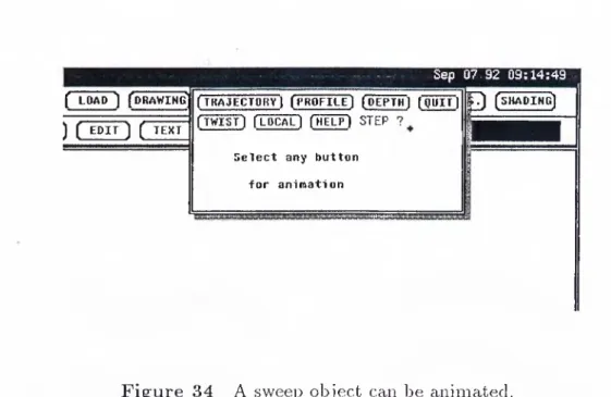
4.2.16 Animation of sweep-based o b je c ts ...49
5 C onclusion 56
List o f F igu res
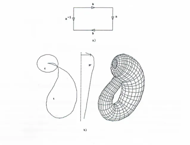
1 The representation of a sphere as a 2-gon aa~^ in topology. A sphere can be represented with two curves (a contour c and a
trajectory t) in Tb... 8
2 A rectangle represented by aba~^b~^ is transformed into a torus via an appropriate identification of the sides... 8
3 A torus can be defined by a contour curve c and a trajectory curve t in Tb... 9
4 A 2-tori is represented as aba~^b~^cdc~^d~^ and can be defined by the appropriate c and t curves in Tb... 9
5 A Möbius strip is defined by a rectangle with baba~^ and by a contour c, a trajectory t, and a twist curve txu in Tb... 10
6 A Klein bottle is defined by a rectangle with aba~^b and by a contour c, a trajectory and a profile curve pr in Tb...11
7 A nonprofiled general sweep object...14
8 A profiled general sweep object... 14
9 Some interactors of the Sunview user interface system... 24
10 General appearance of the user interface system of Tb and some 3-D sweep objects produced by Tb... 25
11 Some improved interactors (for rotation and scrolling)... 27
12 Three example help menus from Tb... 27
13 The number of points on the contour and the trajectory is se lected by the user...29
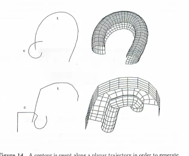
14 A contour is swept along a planar trajectoi’y in order to generate a surface of desired shape. Both curves are defined arbitrarily. . 30
15 The user can create many swept shapes... 31
16 Both of the above objects are obtained by rotating a curve about an axis i (shown in dotted lines). The first curve is a sequence of points, and the second one is a Bezier curve for which a set of control points is given...32
17 Contour c, trajectory i, and depth-modulation zd curves and the produced objects. In the first part, the distance of zd to the axis is constant and the resultant object is a torus. In the second part, this distance is varying and the resultant object is nonplanar... 33 The contour curve is scaled to different sizes (via the curve pr) to obtain a profiled general sweep object...34 Contour c, trajectory i, profile /m, and twist t,w curves and the produced objects. The first object is a profiled object. The second object is a twisted-profiled object... 36 The user can edit the profile and the depth-modulation curves of an object... 37 The user can twist a sweep object... 37 A trajectory curve and some contour curves with different shapes (ci to C5) and the resultant sweep object with varying contour... 38 The user can obtain a sweep object with varying contour. . . . 39 The user can perform 3-D transformations on a sweep object. . 39 Some shading operations and screen dump can be performed. . 41 An image can be translated or scaled... 42 An image or an object can be deleted...42 Special characters can be defined, assigned to any ke}' of the keyboard, and displayed...43 Tb has an interactive painting and colormap changing feature. 44 The user can save or load an object (or an image)... 45 Some blending operations on sweep objects can be performed. . 45 Local deformations on a sweep object. Tb locally deforms the object using di and ¿2 which are the first and the second local deformation curves, respectively...47 A sphere with 120 handles. Symbols show the normalized han dles. For example, H2 oi as — denot es the second handle
obtained by the symbols Oi and uq. (The minus sign is used here
as a synonym for “ ^.) 48
34 A sweep object can be animated... 50 35 Animation by the help of the trajectory curve (c is the con
tour, t\ and ¿2 are the first and the last forms of the trajectory, respectively). Numbers show the animation sequence...51
18 19 20 21 22 23 24 25 26 27 28 29 30 31 32 33
36 37 38 39 40 41 42 43 44 45
Animation by the help of the profile curve (c is the contour, t is the trajectory, and pi and p2 are the first and the last forms of
the profile, respectively). Numbers show the animation sequence. 52 Animation by the help of the depth-modulation curve (c is the contour, t is the trajectory, and zdi and zd2 are the first and the
last forms of the depth-modulation curve, respectively). Num bers show the animation sequence... 53 Animation by the help of twist curve (c is the contour, t is the trajectory, and twi and tw2 are the first and the last forms of the
twist curve, respectively). Numbers show the animation sequence. 54 Local animation by the help of twist curve (c is the contour, t is the trajectory, and twi and tiV2 are the first and the last forms
of the twist curve, respectively). Numbers show the animation sequence... 55 Some rotational sweep objects. The objects are represented with a contour curve and a radius in Tb. Each picture was computed by Tb in about 3 seconds after the initial design of the figures. 59 Some nonprofiled sweep objects. The objects are presented with a contour and a trajectory curve in Tb. Each picture was com puted by Tb in about 4 seconds after the initial design of the figures... 60 Some profiled sweep objects. The objects are represented with a contour, a trajectory, and profile curve in Tb. Each picture was computed by Tb in about 4 seconds after the initial design of the figures...61 Some depth-modulated sweep objects. The objects are truly 3-dimensional and are represented with a contour, a trajectory, and a depth-modulation curve in Tb. It is the depth-modulation curve that gives the third dimension to the trajectory. Each picture was computed by Tb in about 4 seconds after the initial design of the figures...62 Some twisted sweep objects. The objects are represented with a contour, a trajectory, and a twist curve in Tb. Each picture was computed by Tb in about 5 seconds after the initial design of the figures...63 Some sweep objects deformed locally. Each picture was com puted by Tb in about 5 seconds after the initial design of the figures... 63
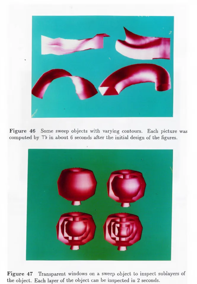
46 Some sweep objects with varying contours. Each picture was computed by Tb in about 6 seconds after the initial design of the figures... 64
47 Transparent windows on a sweep object to inspect sublayers of the object. Each layer of the object can be inspected in 2 seconds... 64
48 Some objects produced by composing the sweep objects. Each picture was computed by Tb in about 7 seconds after the initial design of the figures...65
49 Some familiar objects produced by composing sweep objects. Each picture was computed by Tb in about 6 seconds after the initial design of the figures... 66 50 A punctured surface of genus 4. The picture was computed by
Tb in about 10 seconds after the initial design of the figure. . . 66 51 Projections of a knot (digitized from [25, p. 150])...67 52 Projections of a knot. The picture was computed by Tb in about
40 seconds after the initial design of the figure...67
53 A knot (the first figure digitized from [25, p. 38] and the sec ond produced by Tb in 6 seconds after the initial design of the figure)... 68
54 Swapping handle cores (digitized from [25, p. 140])... 69 55 Swapping handle cores. This picture was computed by Tb in 1
minute after the initial design of the figure... 70
56 Eight knot (the first figure taken from [25, p. 37] and the second produced by Tb in 20 seconds after the initial design of the figure)... 71
57 A picture of a statue rendered from wood (taken from [27, p. 87])...72
1
In tro d u ctio n
A free-form surface modeler offers a set of surface design tools of which one can distinguish three types: constructors, modifiers, and combiners [21]. Construc tors present several methods for generating 3-D models of (real or imaginary) objects. The most popular approach is to use polygons as low-level building blocks which define increasingly complex objects. For example, thousands of polygons might be used to approximate a wine glass [11]. Obviously, it is difficult and time consuming for a designer to define an object in this way. Therefore, a constructor must include higher level capabilities, such as the de scription of a surface by interactive positioning of the control points or by a surface-fitting operator using interpolation or approximation. One objective of this class of tools is to allow the design of desired surfaces to be performed as simply as possible. Hence, a capability to define generic constituents described by a few parameters is very useful. The constituents can be ordinary (a sphere, a torus, a box) or more complicated (a surface of revolution). Sometimes it is necessary to use a higher level component such as a B-spline (or a Bezier) surface. Such surfaces or parametric patches require numerous calculations when it comes to rendering, although they can be represented in a compact form [12, 13, 14, 23, 24, 34].
Modifiers change the shape of an existing surface. The simplest technique is to move (or add) some control points, but more advanced operations have also been developed. For example, tapering, twisting, and blending techniques are available for smoothing and deforming a surface according to continuity constraints [50]. Finally, combiners are Boolean operators applied to the sur faces designed via constructors and modifiers. Each of these three operators has proved beneficial and therefore a modeling system should provide a gen
In this thesis, the suggested techniques for modeling 3-D shapes are all based on sweeping. We give interactive methods for specifying and manipu lating 3-D representations and discuss the desirable functionalities of an inter active graphics system to visualize the complicated shapes of low dimensional topology and knot theory [22, 37, 41, 56]. The implemented program Tb (‘Topologybook’) is a rudimentary graphical workbench* to help topologists (also artists, solid modelers, publishers, and geographers) to illustrate their ideas more effectively. Tb was implemented in the C programming language [38, 39] and runs on a color Sun^ workstation.
Our research owes its existence to A Topological Picturebook [25] of George K. Francis—a book that was written to encourage topologists to illustrate their work and to help artists to understand the abstract (and invariably difficult) ideas expressed by such drawings. The reader is referred to references [2, 3, 4] for early origins of the present work (alljeit from a geometrical viewpoint) and related ideas. Other relevant contributions on the theme of this thesis can be found in references [15, 48, 49].
Indulgence in a topological ‘picturebook’ may sound somewhat futile vis-à- vis the trend that sketching and visual presentation of topological constructions (and proofs) are slowly losing their stronghold which they once held. It may appear that the science of the ‘deformation of shapes’ is becoming sterile in terms of figures. However, we believe that there is definite place for a topo logical picturebook of the sort to be described hei’e (also cf. [22, 37]). The following excerpt [25, p. 78] succinctly explains our view:
“[T]he pedagogy that underlies the entire book, and which I bring out specially here, comes from Bernard Morin of Strasbourg. Pic tures without formulas mislead, formulas without pictures confuse. I don’t know if Bernard would say it this way, but it is how I have understood his work . . . Morin’s vivid, pictorial description of his bold constructions has inspired their realization in many a drawing, model, computer graphic, and film. But he insists that ultimately, pictorial descriptions should also be clothed in the analytical garb of traditional mathematics.”
An outline of the thesis is as follows. In Chapter 2, a brief topological review will be presented. In Chapter 3, sweeping is illustrated and a matheinatical model of general, profiled, depth-modulated, and twisted-profiled sweep ob jects is given. A new model of twisted-profiled general sweep objects with a
(possibly varying) contour can also be found in this chapter. In Chapter 4, the implementation of Tb is illustrated. (The reader is referred to Appendix A for technical details of Tb software.) Here, the user interface system of Tb and modeling, editing, and local or global deformations of sweep objects are presented. In addition, ruled curves, skinning, and blending of objects are covered. Handle normalization, shading, transparent windows on objects, transformations, text and image operations, animation of sweep-based objects are also presented in Chapter 4. Finally, in Chapter 5, a conclusion is offered and some limitations of Tb (along with a description of future work) are listed.
2
T opological R ev iew o f
Tb
In this chapter, we briefly compare symbolic forms of some polyhedra in topol ogy and their curve representations in Tb. The reader will find in Section 2.1 coverage of the standard representation of 2-manifolds. Essentially, the trans formation of a surface from a symbolic form to a visual representation is where we use sweeping as a modeling technique. This point will be made clearer in Section 2.2.
2.1
N o rm a l Form s for Surfaces
Suppose we are given a surface made of (say) rubber. If we distort it in a continuous manner without tearing it, the resulting surface will have the same chromatic num berf Similarly, if a graph (which we may imagine to be made of wire) is distorted without tearing, many of the properties of the graph remain unchanged [27, 53, 56]. The study of those properties of a figure which do not change after deformation is a main concern of topology. It is useful to give a precise mathematical definition of the kind of deformation we have in mind, viz. a homeomorphism.
Let E and F be point sets in Euclidean 3-space. Assume that for each point X E E there exists a corresponding point f { x) G F and for each point y G F there exists exactly one point x G E such that /(x ) = y. Such a mapping / from F to F is called a J-J correspondence. The inverse transformation which leads from each point y ^ F back to the original point x G F is denoted by
and we write f~^{y) = x- A transformation f of E onto F is defined to be continuous at a point Xo of E, if for each £ > 0 there exists a i > 0 such that for every x £ E with a distance less than 8 from .To, the distance between f { x) and / (to) in F is less than £. If / is continuous at each point of jB, we say /
is a continuous transformation of E onto F. If / is a 1-1 correspondence of E onto F and / and are both continuous, then / is called a homeomorphism. If there exists a homeomorphism of E onto F, then E and F are said to be homeomorphic and F is said to be the topological image of E. Some examples of pairs of homeomorphic figures are as follows:
• A circular disk, a square.
• The surface of a sphere, the surface of a tetrahedron. • The interior of a circle, the interior of a rectangle.
• A set of n distinct points, another .set of n distinct points. • The surface of a torus, the surface of a tea cup.
• A solid torus, a tea cup.
A circular disk is the surface (the interior and the circumference) of a cir cle. Each topological image (in 3-space) of a circular disk is called a 2-cell. Similarly, the topological image of an edge is called a 1-cell. Consequently, a 0-cell is just a point. By the term ‘polygon’ (triangle, quadrilateral, pentagon, hexagon, etc.) we do not restrict ourselves to plane figures. We define a poly gon with r sides (an r-gon) as a 2-cell which has its circumference divided into r arcs by r vertices. The arcs are the sides of the polygon.
Given a finite number of polygons, let the total number of all of the sides of the polygons be even. These sides are given in pairs and are labeled. Two sides of a pair are labeled with the same letter. It is furthermore supposed that for each side an orientation is given (say, indicated by an arrow). Identifying each pair of sides such that the arrows coincide (i.e., point in the same direction) if one obtains a connected pseudograph consisting of the vertices and the edges (superimposed sides), then the figure so obtained is a polyhedron. The faces
The plane representation of a polyhedron is all the information that have been mentioned so far: the polygons, the pairing of the sides, and the orienta tion of the sides (before identification). A symbolic description of a polyhedron is created in the following way. For each polygon in the plane representation, choose an orientation. Then, for each polygon, write down the cyclic order of the sides as a row of the corresponding labels (put a minus sign after the label if the orientation of the polyhedron is opposite to the orientation of the side). As a result a scheme (denoted by S)
-1
is obtained with the following ])roperties: (i) Each letter appears exactly twice in E, and (ii) The set of the rows in S cannot be separated into two disjoint subsets such that property (i) holds for each of these subsets. The following operations change E (but not the polyhedron it represents): (i) Put the first letter of a row behind the last letter, (ii) Whenever a certain label appears, say a, replace it with (and a~^ with a), and (iii) simultaneously change all the signs in a row and reverse the cyclic order.
To get a general idea about all possible kinds of polyhedra one proceeds as follows. Given a polyhedron P and its symbolic representation scheme E, one defines four elementary operations. The propert}' of these operations is that although they change P as well as E, the surface itself is not changed. The elementary operations are as follows:
• SUl (Subdivision of dimension one): An edge of the polyhedron is di vided into two new edges by taking an inner point of the edge as an additional vertex.
• COl (Composition of dimension one): Inverse of SUl.
• SU2 (Subdivision of dimension two): Two vertices of a polygon in the polyhedron are connected by a new edge dividing the polygon into two new polygons. •
Two polyhedra P and P' are said to be elementarily related if P can be transformed into P' by using a finite number of SUl, COl, SU2, and C02. A polyhedron is orientable if one can choose an orientation for each polygon such that each edge is used in both possible directions. The alternating sum E( P) = o;o — cfi + 012 for a polyhedron P is called its Euler characteristic. Here « 0, cvi, and o;2 denote the number of vertices, edges, and polygons, re spectively. (In S, «2 = the number of rows and o-i = the number of different letters.)
It turns out, by the fundamental theorem of the classification of 2-manifolds [53], that each polyhedron is elementarily related to one of the following nor mal forms: (Ho) (H,)
(c,)
.-1 a a ÜI bi Cl Cl C2 C2 «P K % ^ K ^Hq is the normal form for a sphere (Euler characteristic = 2). Hp is the
normal form for a p-tori, p = 1 ,2 ,... (Euler characteristic = 2 — 2p). Finally, is the normal form for a nonorientable surface (Euler characteristic = 2 — q, 9 = 1 ,2 ,...).
2.2
S im p le T o p ological S hap es in Tb
Consider a rectangle and assign a definite sense of direction (orientation) to the perimeter. Denote the sides by a, 6, a, b in that order. Place an arrow on each side such that the two sides a (or b) are made to coincide and such that the heads of the arrows coincide as well. The “row”
aba ^b ^
is considered as a symbolic description of a polyhedron (e.g., a torus). It represents the four sides of the rectangle. The notation a~^ in above formula means that the third side is denoted by a but its arrow points opposite to the given orientation of the rectangle. As another example, consider a lune, i.e., a polygon with only two sides. Put arrows on the two sides such that the symbolic row reads
F ig u re 1 The representation of a sphere as a 2-gon aa ^ in topology. A sphere can be represented with two curves (a contour c and a trajectory t) in Tb.
F ig u re 2 A rectangle represented by aha ^6 Ms transformed into a torus via an appropriate identification of the sides.
This defines a division of the sphere into just one lune. That is, a sphere can be represented in topology as aa~^ and this is equivalent to a 2-gon (cf. Figure 1). A sphere can be represented in Tb by the help of two curves (a contour curve c and a trajectory curve t).
A torus can be denoted aba~^b~^ as a symbolic representation and with a rectangle as a topological representation. Figure 2 shows the representation of the torus as a rectangle and prescribes how it can be constructed by the help of the rectangle. Figure 3 shows the representation of the torus by the help of the contour and the trajectory curves. Figure 4 depicts the represen tations of 2-tori in topology and Tb. Symbolic representation of a 2-tori^ is aba~^b~^cdc~^dr^.
F ig u re 3 A torus can be defined by a contour curve c and a trajectory curve t in T k
F ig u re 4 A 2-tori is represented as aha ^cdc ’ and can be defined by the appropriate c and t curves in Tb.
There are also polyhedra which cannot be embedded in 3-space without penetrating themselves. Consider a rectangle with the symbolic row
baba~^
as in Figure 5a . If we first make the identification along the sides labeled 6, we get a Möbius strip [53]. Figure 5b shows the curve representation of a Möbius strip in Tb. The contour curve c is twisted by the twist curve tw while it is swept along the trajectory curve t.
-1 V b a) 0 3B0 I I I I i I I i I I I I I i tu b)
F ig u re 5 A Möbius strip is defined by a rectangle with baba ^ and by a contour c, a trajectory t, and a twist curve tw in T k
b)
F ig u re 6 A Klein bottle is defined by a rectangle with aba and by a contour c, a trajectory t, and a profile curve pr in Tb.
(Figure 6a), we obtain a tube for which the two end circles are denoted by b. But to identify the two end circles, it is necessary to match the arrows on them. Deform the tube so that one of the ends is somewhat smaller than the other and penetrate this smaller end through the wall of the tube. Then bend the larger end a little toward the interior and the smaller end a little toward the exterior, and attach them according to the required mode of identification. We are left with what is commonly known as a Klein bottle [22, 37, 53].
Figure 6b shows the curve representation of a Klein bottle^ in Tb. The contour curve c is scaled by the help of the profile curve pr while it is swept along the trajectory curve t.
^More complicated topological objects, e.g., an eight knot [25], can be obtained by using contour, trajectory, profile, depth-modulation, and twist curves, ruled curves, skinning, and blending operations in Tb (cf. Chapter 5).
3
T h e Sw eep P arad igm
3.1
A n In tro d u ctio n to S w eep in g
A class of solids called nonproRled sweep objects is defined by two parametric curves: a 2-D contour (cross-section) and a 3-D trcijectory [18]. The contour is moved along the trajectory to generate a parametric surface. A classifica tion of sweep objects is given by Choi and Lee [20]. Another classification is given by Bronsvoort, Nieuwenhuizen, and Post [18]. Here, we prefer the latter because it is more convenient for our purposes.
Sweep objects can be defined in increasing complexity as follows:
• Translational sweep: The contour is arbitrary and the trajectory is a straight line.
• Rotational sweep: The contour is arbitrary and the trajectory is a circle. • Circle sweep: The contour is circular and the trajectory is arbitrary. • General sweep (generalized cylinder): Both the contour and the trajec
tory are arbitrary. This can be classified as: — Nonprofiled general sweep,
— Profiled general sweep,
- Depth-modulated general sweep, and - Twisted-profiled general sweep. Here, only general sweep will be considered.
3.1.1 N o n p ro filed g en eral sw eep
Nonprofiied general sweep is defined by an arbitrary closed 2-D contour and an arbitrary 3-D trajectory [18, 50]. Here, the 2-D contour c can be defined in parametric form:
c(u) = (c^(u), Cj^(u)) c(ui) = c{vf)
V i < V < V f
As a parameter, v varies from to vj. The parametric functions and Cy trace out the contour. The 3-D trajectory t can be defined in the paramet ric form:
t(u) = (ta;(u), t„(u), t^(u)) U \ < U < Ul
As a parameter, u varies from ui to u;. The parametric functions t^,, tj,, and tz trace out the trajectory. For nonprofiled general sweep, the contour c moves along the trajectory t. (c remains constant along t.)
The spatial relation between the contour and the trajectory must be defined at every point of the trajectory. Figure 7 illustrates a nonprofiled general sweep object. The contour plane is perpendicular to ei, the unit vector tangent to the trajectory. As 63, a fixed unit normal to the plane of the trajectory is chosen. Note that 62 is the vector product of 63 and ej. A profiled general sweep object is given in Figure 8.
Consequently, it is possible to present a nonprofiled general sweep as a vec tor function Tnp of two parameters u and v:
T„p(u,u) = (Sw eep(t(u), c(u))
U\ < U < Ul U\ < V < V j
For the sweep operation, it is necessary to use translation and 3-D rotation. The direction of the tangent vectors for the first and the last points of the trajectory must be selected as directions of the first and the last segments to rotate the contour. For other points, the direction of the vectors as specified by the previous and the next points must be selected [5].
F ig u re 7 A nonprofiled general sweep object.
Other mathematical models of sweep objects are given by Post and Klok [50], Martin and Stepson [44], and Wang [57].
3.1.2 Profiled general sweep
If some deformations are necessary on a nonprofiled general sweep by scaling, then a profiled general sweep can be defined as a mathematical model. The contour can be scaled independently in x and y directions. For each point of the trajectory, two scale factors and Sy are specified. The scale functions are expressed in terms of the parameter of the trajectory:
S(u) = (Si(u), Sy(ti)) Ul < u < Ul
If the scale factor is substituted in T,jp (cf. Section 3.1.1), it will have an effect only on the contour functions and the resultant profiled general sweep will be defined as a vector function Tp:
Tp(u,u) = (Sweep(t(u), c(u)), S(u))
U\ < U < Ui < V < V f
We cite some works on deformation by scaling. Coquillart presents an offset technique [21], Woodward studies the B-spline sweep with scaling [58, 59], and Arslan and Akman offer an interactive scaling technique [5, 10, 7].
3.1.3 D ep th -m od u lated general sweep
Sometimes it is necessary to give a third dimension to the sweep objects in an interactive system. In this case, a mathematical model of a depth-modulated general sweep can be given as a vector function in the following form:
Td(u,u) = (Sweep(t(u), c(n)), D(t^(n)))
Section 4.2.2 gives more information about depth-modulated general sweep objects.
3.1.4 T w isted-profiled general sweep
If the contour curve is deformed by twisting and scaling while sweeping along the trajectory curve, the produced surface is called a twisted-profiled general sweep object. The contour curve can be twisted independently in x and у directions for each point of the trajectory curve. For this purpose, two twist factors Tyjx and can be specified. The twist functions are expressed in terms of the parameter of the trajectory:
M l < U < M(
If the twist factor is substituted in Tp defined in the previous subsection, it will have an effect only on the contour functions and the resultant twisted- profiled general sweep will be defined as a vector function T„,p:
Ti^,p(m,m) = (Sw eep(t(u), c(m)), Tu,(u), S(u)))
Ui < u < Ut < V < VJ
We now cite some works on deformation which influenced our work. Coquil- lart presents an offset technique for control points of rational B-spline curves to produce (profiled) sweep objects [21]. Choi and Lee use simple transforma tions and blending to represent more complex sweep objects [20]. Woodward presents a skinning technique to produce 3-D shapes that resemble blended sweep objects [58, 59]. Finally, Arslan and Akman present new interactive techniques to produce and deform sweep objects [5, 6, 7, 8, 9, 10, 11].
3.2
A D isc r e te M o d el for S w eep in g
A sweep surface Sw(C, T) is produced by moving a given contour curve (7 along a given trajectory curve T. The plane of C must be perpendicular to T at any point of T. C may be any planar closed or open curve and T may be any 3-D closed or open curve. If Cis a closed curve and Tis a 3-D curve segment, then the produced sweep object is called a generalized cylinder [21].
If C is deformed by scaling with a scale factor as it is swept along T, then the produced sweep object is called a profiled general sweep object. Here, we accept as the scale factor the distance of a given curve P to any selected axis. So, a profiled general sweep surface can be defined as Swp(C,T,P). Here, P represents a profile curve which is the same number of points with T.
If C is deformed by twisting and scaling while sweeping along T, the produced object is called a twisted-profiled general sweep object. We define the twist factor by a curve Tw. This is a planar curve which has the same num ber of points with T and is mapped between the minimum and the maximum values of the twisting angles only at one dimension. Then, a twisted-profiled general sweep surface can be defined by four curves, viz. Sukp(C,T,P,Tw).
In the following subsections, we present a discrete mathematical defini tion of twisted-profiled general sweeping. In this definition, we use the conven tional matrix notation^l to represent the transformations and obtain a general sweep matrix as a result. In our representation, the matrix twists, scales, and sweeps a contour curve C along a trajectory curve T to handle a grid of general sweep surface points. We will formulate the discrete mathematical definitions of curves {C, T, P, Tw) as vector functions.
C is a planar curve or polygon with n points and each point (a;,·, ?/,·, 0) of C can be represented as Q, ¿ = 1 , 2 , . . . , n. T is any 3-D curve or polygon with m points and (without loss of generality) the first point of T is in the origin. Each point {xj, yj, Zj) of T can be represented as Tj, j = 1, 2, . . . , m. P can be given as a 1-D position vector with m component vectors that include scaling factors. But here, we take P as a planar curve and later calculate the scaling
IISome matrix representations for sweeping are given by Rogers and Adams [54]. But, these are restricted and work only for given planar curves and situations that depend on curve equations.
factors by the help of the curve. This may be useful for interactive systems. Each point (xj, yj, 0) of P can be represented as Pj, j = 1 , 2 , , m. Tw can be also given as a 1-D position vector with m vectors that include twisting factors. We choose to specify Tw as a, planar curve and later calculate the twisting factors by the help of the curve. Each point (xj,yj,0) of Tw can be represented as Twj, j = 1 ,2 ,... ,m.. In the sequel, we give a procedure to handle a twisted-profiled general sweep object. In this procedure, C is a curve centered at the origin and the first point of T is also at the origin. In other cases, they must be translated to origin and then the generated curves must be translated back to their actual positions at the end of the procedure. First, (7 is rotated around the 2;-axis by Tw for twisting. Second, (7 is scaled by P. Third, (7 is rotated around the x, y, and 2-axes by angles found for each point of T. Finally, each twisted, scaled, and rotated C is translated to every point of T.
3.2.1 T w istin g
We have taken the twisting factor Ttu as a ])]anar curve. But, Txu represents only the twisting angles for each point of the trajectory curve T. That is, it can be represented as a 1-D vector function linearly interpolated at only one dimension of Tw. Tw can be drawn interactively as a planar curve in an in teractive system and then is interpolated at one dimension to handle twisting angles (cf. Section 4.2.4 for details). The interpolated TD vector function 6 includes rotating angles for each point of T and can be shown as follows 0·^ j = 1 , 2 , .. . ,m. The following matrix rotates a contour curve C that is centered at the origin (for twisting as a function of 0)\
P,t w c6j sOj 0 0 ■ - s 0 j cOj 0 0 0 0 1 0 0 0 0 1 cOi ^ cos Oi a D f . a sOj = sinffj 3.2.2 Scaling
We have taken a profile curve P (a planar curve) as the scaling factor. P also represents only one magnitude for each point of the trajectory curve T. Then,
it can also be written as a 1-D vector function which takes the distances of the vertices of P to the vertical (or horizontal) axis at only one dimension. For an interactive system, first, an axis is given for reference and P is drawn interactively. Then, distances of vertices of P at one dimension to the axis give the scaling factor for C. Scaling factor s is a 1-D vector function and in cludes scaling radii for points of T. It can be shown as Sj, j = 1, 2, . . . , m. The following matrix scales a contour curve C that is centered at the origin, as a function of s: Sj 0 0 0 0 0 0 0 0 Sj 0 0 0 0 1 3.2.3 R otation
The twisted-profiled contour curve C must be rotated in 3-D with respect to the tangent vector at each point of trajectory curve T. That is, the plane of C must be made perpendicular to the tangent vector of T at each point. We calculate the discrete derivative for each point of T to handle the tangent vector. To this end, we add two dummy vertices To and T„i+i to T. (To = T\ and Tn+i = T„j.) In the following, we use matrices Ra;,Ry, and R- to handle the real position of C and Tx, Ty, and Tz to represent the x, y, and z distances of the vertices of T.
Rotation around the a:-axis:
1 0 r D 1 _ 0 caj [ ^ ^ \ - 0 - s a j 0 0 SOij caj 0 0 0 0 1 D f caj = cos aj = D j . scv,· = sm a,· = Tyj-i-Tyj+i /lx /lx = y ( T % _ i - T y , + i ) 2 + (Tzj_i - TZj+rT· Rotation around the y-axis:
Ry j — c^j 0 —s0j 0
0
1 0
0
s^j 0 c[)j 0 0 0 0 1 CD ¡ W C O S 0 Í = sD X sin f t =hy = ^/{Txi-, -
Rotation around the 2r-axis:
Rz cij 57i 0 0 s - f j cjj 0 0 0 0 1 0 0 0 0 1 C7j = cos 7j = S ^ , ? / s ill = I m i l I l U = L — \ / — 1 ^^V+i)” "t (^2/j-i ^ 2/j+1)” 3.2.4 Translation
Finally, C must be translated to each point of T to finish the sweeping opera tion. We use a 3-D translation matrix as follows:
T X x y z ■ 1 0 0 0 ■ D J 0 0 1 0 0 1 0 0 a = h ^ d D J a b c 1 c =
3.2.5 O btaining th e m atem atical m odel
A general twisted-profiled sweeping matrix Swtp is obtained, if the above transformation matrices are multiplied in the following order:
Swtp = R,tw S' Rx Rv Rz Tx y z
[ S w tp ] =
Sj cOj c/3j cjj SjcOjc0jSyj -SjcOjS0j -\-Sj sOj saj s/3j cjj +5; s6j saj spj sjj -{-Sj sOj saj cpj 0
—SjsOjcajSjj +Sj s9j caj cjj
-Sjs9jC0jCjj —Sj sOj cpj sjj Sj sOj spj cdj saj s(3j cjj -{■Sj cdj saj spj sjj -i-Sj cOj saj cpj 0 — SjCOjCOCjSJj -\-Sj cOj caj cjj
Sj caj sPj cjj Sj caj spj sjj
-\-Sj saj sjj —Sj saj cjj Sj caj cpj 0
a b c 1
Consequently, a twisted-profiled sweep surface can be calculated in the fol lowing form. First, each point of C must be evaluated for matrix Swtp, and then, a new matrix Swtp must be modified for each incremented j.
Sweep surface C SwHp
j,6,s I < i < n 1 < j < m In the above formula, j varies slowly, i.e., we compute the formula for a par ticular j and every i.
For the planar case, if (7 is a 2-D curve or a polygon centered at the origin in the x-y plane and T is a curve or polygon starting at the origin in the x-z plane, then a planar twisted-profiled sweep surface can be computed with the help of following matrix:
Sw.ptp яtw .5; Rb Tx z
After some manipulations, the following is obtained:
[ 'ptp J
-Sjcdjcfj SjsOj —sjcdjsfj 0 —Sjsdjcfj SjcOj Sjs9jS0j 0
SjS0j 0 SjC0j 0
a 0 6 1
3.2.6 Sw eeping w ith varying contour
A twisted-profiled sweep surface can be calculated in the following form. First, each point of C must be evaluated for matrix Swtp, and then, a new matrix
Swip must be modified for each incremented j :
Sweep surface C SwHp
j,6,s 1 < f < n 1 < y < m
In the above formula, j varies slowly, i.e., we compute the formula for a particular j and every i. The contour curve C is a constant curve along the trajectory curve T. But frequently C must be a different curve for some points of T to handle more complex sweep objects. Our approach to resolve this situation is as follows.
First, different contour curves are defined for some points of T. Second, these curves are linearly interpolated respectively to obtain new contour curves for each point of T. Third, the obtained 2-D discrete curves are used for the sweep operation. (That is, a different contour curve is used for each point of
T to obtain sweep surfaces with varying contour.)
A twisted-profiled sweep surface with varying contour can be calculated in the following form:
Sweep surface with varying contour
i,k,j,0,s
C
i,k Swip
\ < i < n 1 ^ j , h < m In the above formula, a diffei’ent contour curve is taken into account for each point of the trajectory curve.
4
Softw are C h aracteristics o f Tb
4.1
U ser In terface o f Tb
A good interactive modeling system must have an enjoyable and powerful user interface. In this section, the user interface system of Tb and some ideas on which the system is based will be presented.
4.1.1 U ser interface system s
The following short descriptions may be useful;
• User interface management system: A user interface management sys tem (UIMS) is a tool set designed to encourage cooperation in the rapid development, tailoring, and management of the interaction in an appli cation domain across varying devices, interaction techniques, and user interface styles [42].
• User interface system: The combination of window-based displays, menus, icons, and a mouse that is increasingly used on personal com puters and workstations. •
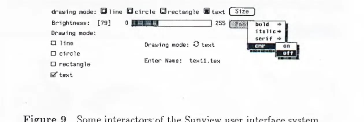
• Interactors: They are elements that are presented to the programmer by user interface systems and play an effective role to provide user computer interaction. In general, interactors include the following elements:
— windows,
— pulldown menus, — buttons,
— mouse, light pen, and other pointing devices, — scrollbars,
— etc.
Figure 9 shows some interactors of the Sunview** user interface system.
255 draujing mode: Q l i n e 0 circle 0 rectangle 8 text [ Size Brightness: [79] 0
Drawing mode:
^ Drawing mode: C text
□ circle
r-1 . , Enter Name: textl.tex U rectangle
text
b o ld i t a l i c s e r i f
F ig u re 9 Some interactors of the Sunview user interface system.
• Dialog: A sample user interface, or part of a com2Dlex user interface, can be realized by a small, fixed collection of interactors. Such a collection is called a dialog [19].
4.1.2 U ser interface design of Tb
As we have mentioned in Section 4.1.1 a user interface management system presents a set of user interface components to programmers. In general, these components are called interactors (windows, menus, scrollbars, buttons, text areas, mouse, and so on). A programmer must only perform a suitable orga nization of these interactors. In other words, a programmer must build a user interface system by using events, states, or attributes of the supplied interac tors.
A good user interface system must have the following properties [39]:
• Ease of use and naturalness • Speed and effectiveness
• Elegance and enjoyable features
Tb has a rather straightforward user interface. Figure 10 shows the general appearance of this interface.
06 92 14:31:07 ["qUIT^ ['gRID^ ( SAVE ] fcOLORIHG^ f LOAD j ^DRAWING] ['XFORM^ f ERASE ] ^TOPOLOGY] [IMAGE OPS.j [SHADINg'] [ TWIST ] [blending] [local,def. ] [ EDIT ] [ TEXT ] [skinning] [animation]
F ig u re 10 General appearance of the user interface system of Tb and some 3-D sweep objects produced by Tb.
Of course, the main goal of a user interface system must be to provide the above requirements. But Tb is a research tool and sometimes, speed is pre ferred over comprehensibility and orthogonality. Tb’s user interface is based on the following guidelines:
Interactors with major functionality are shown on the screen all the time. Some interactors with similar purposes were collected together. They were designed as buttons and placed in the top side of the main window. They are continuously shown on the screen so that the user immediately can activate any of them.
• Excluding text operations, only the mouse is used for interactions. In teraction time is important in our system; interaction must be provided in the shortest way. Using mouse was thus usually preferred over the keyboard.
• It is made sure that the interactors do not occupy too much space on the screen. The working area must be fairly wide and the user interface area must be fairly scant in a graphical interaction system.
• Interactors and their positions are good-looking and well-placed. Differ ent colors, shapes, and fonts have been used for interactors to decrease the accommodation time of the user. The position of interactors must be in the adequate form. For example, consider the button DRAW to
construct an object. Many submenus are shown to select the drawing type. After constructing the object, the button SHADING will be selected from the main menu to shade the object. If SHADING is overlapped with
DRAW, it would be problematic to select SHADING.
• It is made sure that the interactors have not too many items. For exam ple, it can be time consuming to choose the necessary items if a menu has many items. For this, menus with small sizes and few items must be designed to decrease the accommodation time. For example, consider a menu which has eight different drawing items and five different shading items. User has to select any of the 13 different items. If shading is not necessary at that moment, five items occupy space on the screen.
• To increase the speed of the system, sometimes interactors with a special purpose are defined. Figure 11 shows some rotational interactors in Tk • Some dynamic menus can be improved instead of using the keys of the
keyboard. For example, loading is performed dynamically in Tb. The saved file names are shown immediately by color menus on the screen. User must select a file name to load it.
• There are two types of help menus used in Tb. In the first type, help menus are resident and tell the user what they will do. In the second, each interactor has its own help text which flashes or beeps to warn the user. Figure 12 gives some examples.
( ROTATE J [TRANSLATE] [ SCALE ) [ ROTATE OBJECTS ) [ QUIT ] [ HELP J
Use the left button
Select an angle for rotation.
- m
[ t w i s t ] [q u i t] [HELP] 1 ( ROTATE ) [TRANSLATE] [ SCALE ) Use the left button 1 [ ROTATE OBJECTS ] [ QUIT ] ( HELP )
S
1
Use the left button Select a scaling coefficient
B B S M i B H i
Select an angle .... --...
F ig u re 11 Some improved interactors (for rotation and scrolling).
[Number of s y m b o l s ^ ^ [ QUIT J [ HELP ]
Give a number to determine the number of handles
[ LOAD NORMAL ) [ LOAD RASTER ] i QUIT ] [H K IIO ·!·;
Inage files are loaded froo the directory '^Draster^
Normal files are loaded fro« the directory '‘Dnormal'
Contour points Trajectory points ? ( QUIT 1 [ H E L P 1
Enter tuo numbers to determine the number of points on the contour and the trajectory.
4.2
A v a ila b le F u n ctio n a lities
The implemented program Tb can be regarded as an interactive mathematical picture ‘modeler’, ‘constructor’, ‘shader’, and ‘animator’. It is also useful for solid modeling [32, 33, 43, 52, 61]. The interaction of Tb with the user is straightforward. For example, a torus can be rendered by selecting only five control points to produce the contour and a radius. Our fundamental aim is to hide the details of the processing from the user. This is in the precise spirit of Pentland’s sketching system [48, 49]. The main goal of our work is to provide a rudimentary grai^hical workbench to help topologists, artists, solid modelers, and geographers to illustrate their ideas more effectively. An auxiliary goal is to improve publication-quality production of mathematical figures.
In this section, the power of Tb is presented. A general appearance of main interactors of Tb is shown in Figure 10. Each interactor has many subinter actors. Therefore, each main interactor of Tb is given as a subsection and the respective submenus are presented in some detail.
4.2.1 Grid selection
We are interested in discrete sweeping and accordingly, every curve used in Tb is considered to be a sequence of discrete points.
A general sweep object is represented by two curves (contour and trajec tory) in Tb. Contour and trajectory curves usually have many discrete points. The number of points on the contour and the trajectory curves determines the number of grids of the produced sweep object. So, the number of discrete points in auxiliary curves must be determined by the user. Menu GRID (cf. Figure 13) lets the user select this number.
The profiled, depth-modulated, and twisted sweep objects have a profile, a depth modulation, and a twist curve, respectively. The number of points on these curves is set automatically to the number of points of the trajectory curve. The help menu gives information about how the selection is done and how many points there are on the contour and the trajectory curves.
Contour points Trajectory points ?
( Tw:
[ QUIT 3 [ HELP ]
Enter two numbers to determine the number of points on the contour and the trajectory.
(d r a w i n g]
F ig u re 13 The number of points on the contour and the trajectory is selected by the user.
4.2.2 D raw in g
In this subsection, we present some interactive methods to produce swept shapes. For each method, curves are specified and drawn interactively by the help of a mouse. They can be produced in two ways: free form and approxi mated form. In the former, a curve is produced by entering points of the curve by the mouse. There is no further operation to smooth the curve. In the latter, a curve is produced by entering each control point of the curve by the mouse. In this case, the curve is approximated with the use of Bezier or B-spline [17, 18, 19, 20, 21, 22] algorithms (and the produced curve is smooth).
The following sweep objects can be created by the help of drawing menu: • Rotational sweep objects
• Nonprofiled sweep objects • Profiled sweep objects
• Depth-modulated sweep objects • Twisted-profiled sweep objects • Assorted knots
In the following. We only give directions for creating a nonproiiled sweep ob ject in detail by using the button DRAWING. Each of the other objects can be
created via similar selections.
Inputs to produce a nonprofiled sweep object are two curves. The output is a 3-D object obtained by moving or sweeping one curve along the other (cf. Figure 14). The method includes both translational and rotational sweep and provides the user with an opportunity to create complex 3-D objects. Curves that are sequences of points in space are stored in a 1-D array in Tb. They can also be determined in any other way such as a B-spline method or by inputting a sequence of 2-D points. One curve is considered to be a path on which the
F ig u re 14 A contour is swept along a planar trajectory in order to generate a surface of desired shape. Both curves are defined arbitrarily.
other curve moves while generating a surface. The main idea of the method involves two transformations, namely a 3-D translation and a 3-D rotation. The first curve is replicated on the second curve by translating the contour to the points of the trajectory as many times as the number of points given for the trajectory. In other words, one copy of the contour curve is generated
for each point of the trajectory curve and is moved to these points. Next, the replicated curves are rotated by the position of the point.
The user must select the button DRAWING to produce a sweep object. After the selection of the button, the menu that is shown in Figure 15 is displayed. User must select the button NONPROFILED SWEEP to create a non- proiiled sweep object. Some submenus such as FREE_FREE, FREE_BEZIER, BEZIER-FREE, and BEZIER-BEZIER are shown on the screen. The button
BEZIER-FREE inform that the contour curve will be drawn by using the Bezier algorithm and the trajectory curve will be drawn as a free form curve. After the selection of any menu, the contour and the trajectory curves of the nonpro- filed sweep object is drawn. As a result, Tl· uses curves to create a nonprofiled sweep object.
Qi
[ ROTATIONAL ] [ DEPTH-MODULATED t NOHPROFILED ] ^PROFILED MDDULATEdI
PROFILED ] ( KNOT ] [Q U Ilj [HELP S e le c t draw ing type
FREE.FREE FREE.BEZIER
BEZ1ER.DEZ1ER
F ig u re 15 The user can create many swept shapes.
The second interactive method to produce swept shapes is well-known and commonly called simple rotationa.1 sweep. Let p be a point in 3-D. If p is rotated about an axis I the resultant figure is a circle in 3-D. Similarly, if one takes a line segment s and rotates it about I a cylindrical object is obtained. Now, take a circle c and rotate it about 1. The resultant figure is a torus (cf. Figure 16). Mouse-picked control points are used to define an arbitrary curve segment which in turn is rotated about i. Many interesting surfaces of revolution can be computed in this way.
Although the above methods are restricted to 2-D curves, they can be extended to the 3-D case. For this, we give a third method called nonplanar
5
F ig u re 16 Both of the above objects are obtained by rotating a curve about an axis i (shown in dotted lines). The first curve is a sequence of points, and the second one is a Bezier curve for which a set of control points is given.
general sweep. An important aspect of the method is to enter the 3-D points by the help of a mouse. This is provided by a third curve, appropriately called a depth-modulation curve. The curve gives a nonplanarity to the trajectory and now, the second curve is exactly a 3-D curve (cf. Figure 17). Some knots [22, 37], spirals, and other nonplanar complicated objects can be produced by the help of this method.
zd
F ig u re 17 Contour c, trajectory t, and depth-modulation zd curves and the produced objects. In the first part, the distance of zd to the axis is constant and the resultant object is a torus. In the second part, this distance is varying and the resultant object is nonplanar.
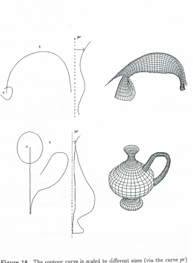
The fourth method is profiled general sweep. Three curves are necessary for this method: a contour, a trajectory, and a profile curve. The contour curve is scaled to different sizes according to the profile curve while sweeping is performed (cf Figure 18).
The last method is a twisted-profiled nonplanar general sweep. Five curves are necessary for this method: a contour, a trajectory, a depth-modulation curve, a profile, and a twisting curve. The contour curve is twisted and scaled
Figure 18 The contour curve is scaled to different sizes (via the curve pr)