T.C.
ISTANBUL AYDIN UNIVERSITY
INSTITUTE OF NATURAL AND APPLIED SCIENCES
THE SIMULATION OF MAGNETIC HYSTERESIS LOOP OF Fe-Sn-B AMORPHOUS ALLOY BY JILES ATHERTON HYSTERESIS MODEL
M.Sc. THESIS
ENGR. MUHAMMAD BILAL YOUNAS
Department of Electrical and Electronics Engineering Electrical and Electronics Engineering Program
T.C.
ISTANBUL AYDIN UNIVERSITY
INSTITUTE OF NATURAL AND APPLIED SCIENCES
THE SIMULATION OF MAGNETIC HYSTERESIS LOOP OF Fe-Sn-B AMORPHOUS ALLOY BY JILES ATHERTON HYSTERESIS MODEL
M.Sc. THESIS
ENGR. MUHAMMAD BILAL YOUNAS (Y1713.300017)
Department of Electrical and Electronics Engineering Electrical and Electronics Engineering Program
DECLARATION
I declare that the information in this document has been obtained and presented in accordance with academic rules and ethical conduct. I also declare that, as required by these rules and conduct, I have fully cited and referenced all material and results that are not original to this work.
FOREWORD
After thanks to Allah our creator, I would like to thank my mother and my father who raised me to become a good person. They were patient during my mistakes and my bad times and helped me in all times and everything I have accomplished is because of their effort. I hope I can make them happy and return even some of what they gave me during their whole lives.
I would like to thank my thesis advisor Prof Dr. EYLEM GULCE COKER for her guidance, support, and help during my work in the thesis. I thank her for everything I learned from her.
I thank all my teachers starting from my school time until today as they had great influence on me and made me love education and I hope I can become one day a good teacher as they were.
September 2019 Engr. Muhammad Bilal Younas (Electrical and Electronics Engineer)
CONTENTS
Page
FOREWORD ... iii
LIST OF ABBREVIATIONS ... vi
LIST OF FIGURES ... viii
LIST OF TABLES ... x ABSTRACT ... xii ÖZET... xv 1. INTRODUCTION ... 1 1.1 Purpose ... 1 1.2 Literature Review ... 1 2. FERROMAGNETIC MATERIALS ... 7
2.1 Magnetization Process in Ferromagnets ... 10
2.2 Electromagnetic fields in ferromagnetic materials ... 12
2.3 Losses in ferromagnetic materials ... 19
2.4 Hysteresis losses ... 19
2.5 MH & BH hysteresis loop ... 20
2.6 Eddy current losses ... 24
2.7 Hysteresis Models ... 26
2.8 Modeling Magnetic Materials... 26
2.9 Theoretical ... 27
2.10 Empirical-conceptual ... 28
3. Fe-Sn-B ALLOY AND JA MODEL ... 31
3.1 Fe-Sn-B Amorphous Alloy System ... 31
3.2 Experimental Details ... 32
3.3 Langevin theory for parameters ... 34
3.4 Jiles Atherton model ... 37
3.4.1 Classic J-A Model ... 37
3.4.2 Modified J-A Model ... 39
4. RESULTS AND DISCUSIIONS ... 45
4.1 Implementation of J-A Model in MATLAB ... 45
vi LIST OF ABBREVIATIONS
JA : Jiles Atherton M : Magnetization EMF : Electro Motive Force Man : Anhysteric Magnetization Mirr : Irreversible Magnetization
viii LIST OF FIGURES
Page
Figure 2.1: Domain Orientation before and after Magnetization ... 7
Figure 2.2: Domain Structure in a Ferromagnetic Material ... 10
Figure 2.3: Magnetization Mechanism ... 12
Figure 2.4: Random Magnetization ... 13
Figure 2.5: Magnetization of a Ferromagnetic Material due to an External Field .... 14
Figure 2.6: Hysteresis Curve Figure ... 16
Figure 2.7: The Energy Essential to Magnetize a Unit Volume of the Ferromagnetic Material. ... 17
Figure 2.8: Energy State of the Hysteresis Loop ... 18
Figure 2.9: Energy Degeneracy Due to the Hysteresis ... 20
Figure 2.10: Ideal Hysteresis Loop ... 21
Figure 2.11: Stabilization of the Loop ... 22
Figure 2.12: Different Serial of Hysteresis Loops ... 23
Figure 2.13: Fundamental Magnetization Curve of Hysteresis Loop ... 24
Figure 2.14: Induced Eddy Currents and Magnetic Counter Field ... 25
Figure 3.1: Hysteresis free Langevin Magnetization Curve ... 36
Figure 3.2: Langevin Diagram ... 42
Figure 4.1: Classical JA B-H hysteresis Loop for Table 4.1 ... 49
Figure 4.2: Classical JA M-H Hysteresis Loop for Table 4.1 ... 49
Figure 4.3: Modified JA B-H Hysteresis Loop for Table 4-1 ... 50
Figure 4.4: Modified JA M-H Hysteresis Loop for Table 4-1 ... 50
Figure 4.5: JA Simulink Model ... 52
x LIST OF TABLES
Page
Table 2.1: Theoretical Models ... 29
Table 3.1: Temperatures ... 33
Table 4.1: Parameters for JA Hysteresis Modeling ... 46
Table 4.2: Parameters for JA Hysteresis Modeling ... 46
xii
THE SIMULATION OF MAGNETIC HYSTERESIS LOOP OF Fe-Sn-B AMORPHOUS ALLOY BY JILES ATHERTON HYSTERESIS MODEL
ABSTRACT
The amorphous alloys have many bases, Fe-B based alloys are the superlative representatives of the traditional metallic glass systems which have many applications according to the soft magnetic features. They have been an extensive research area for periods in the world because of their physical properties and structures. The researches were based on the addition of a diversity of elements into the Fe-B based alloys. There are many methods for determining physically and mathematically the hysteresis curve for soft magnetic materials. Jiles_Atherton theory of ferromagnetic hysteresis is one approach used in transient modeling of electromagnetics. Since the theory introduced several models developed based on this theory. In this article we shall summarize the model that has been implemented and we shall implement a model in MATLAB and Simulink environment for soft magnetic material by two approaches, the classical and modified Jiles-Atherton model. Presented results indicates that the best approach to modeling the magnetic hysteresis loop is with the modified model equation that also corresponds well with the result of physical experimental measurements.
Keywords – Soft Magnetic materials, Amorphous Alloy, Hysteresis loop,
JILES ATHERTON HISTEREZIS MODELİ İLE Fe-Sn-B AMORF ALAŞIM MANYETIK HISTERESIS LOOP SİMÜLASYONU
ÖZET
Amorf alaşımlar birçok bazları var, Fe-B bazlı alaşımlar yumuşak manyetik özelliklere göre birçok uygulama var geleneksel metalik cam sistemlerin üstün temsilcileridir. Fiziksel özellikleri ve yapıları nedeniyle dünyada dönemler için geniş bir araştırma alanı olmuştur. Araştırmalar Fe-B bazlı alaşımlara çeşitli elementlerin eklenmesine dayanıyordu. Yumuşak manyetik malzemeler için fiziksel ve matematiksel histeresis eğrisibelirlemek için birçok yöntem vardır. Jiles_Atherton ferromanyetik histeroz teorisi elektromanyetik lerin geçici modellemesinde kullanılan bir yaklaşımdır. Teoribu teoriye dayalı olarak geliştirilen several modellerini ortaya koyduğundanberi. Bu yazıda uygulanan modeli özetleyeceğiz ve matlab ve Simulink ortamında yumuşak manyetik malzeme için klasik ve modifiye Jiles-Atherton modeli olmak üzere iki yaklaşımla bir model uygulayacağız. Sunulan sonuçlar manyetik histeresis döngü modelleme için en iyi yaklaşım da fiziksel deneysel ölçümler sonucu ile karşılık değiştirilmiş model denklemi ile olduğunu gösterir.
Anahtar Kelimeler - Yumuşak Manyetik malzemeler, Amorf Alaşım, Histerezis
1. INTRODUCTION
1.1 Purpose
By changing the direction of the magnetizing current constantly through the coil from a positive direction to a negative direction, the magnetic hysteresis loop of the ferromagnetic core can be produced. The appropriate selection and processing of magnetic core materials determine the magnetic performance level. The work that was done by the magnetizing force against the internal friction of the molecules of the magnet, produces heat. This energy which is wasted in the form of heat due to hysteresis is called hysteresis Loss. Magnetic research is categorized by the progresses of the mathematical or physical methods based different models. By knowing the hysteresis phenomenon, we have information about on material behavior, for this purpose we must model the hysteresis curve for the material.
The main purpose of this research is to model the hysteresis curves for the ferromagnetic material by JA model due to its closeness with the physical properties of the material. There are many shapes of the model, we tried to choose the best model equation for hysteresis by comparing its original model that developed more than thirty years ago.
1.2 Literature Review
The well-known traditional rapidly quenched nanocrystalline soft magnetic materials for example FINEMET, NANOPERM and HITPERM are currently upheld by new intensely examined systems. Amongst these a special consideration is put on materials with high saturation magnetization whereas preserving low coercivity. Diverse systems based on Fe-B with accompaniments of Co, Cu, C, P, Si and other elements were developed, which achieve necessities on current soft magnetic
2
specifically nanograin size control, is attained by adding Sn into Fe-rich Fe-B system.
Additional investigation of rapidly quenched Fe-Sn-B system has directed to partial replacement of B and Fe by Si and to doping of the base alloy with slight amounts of Cu. Ribbons with changing Si content were set by planar flow casting, directing the foundation of fine-grained structure after controlled annealing. The effects of the replacements and of doping with Cu on stability, Nano crystallization process, subsequent magnetic properties and structure of the moulded phases were studied by thermogravimetry, vibrating sample magnetometry, differential scanning calorimetry, conventional and in-situ x-ray diffraction and transmission electron microscopy. The results will be associated to the performance and structure of the classical nanocrystal-forming systems and the application potential of the new system as soft magnetic material will be evaluated.
The amorphous alloys have many bases, Fe-B based alloys are the superlative representatives of the traditional metallic glass systems which have many applications according to the soft magnetic features. They have been an extensive research area for periods in the world because of their physical properties and structures. The researches were based on the addition of a diversity of elements into the Fe-B based alloys. In the significance of this struggle was the discovery of formation of nanocrystalline phase by restrained crystallization of Fe-B based amorphous alloys which was associated to Fe-Si-B systems. Those stages have importance in considerate the soft magnetic materials behaviours. The effects of addition numerous elements can be found in literature nonetheless a few results have been issued for rapidly quenched Fe-Sn-B ribbons for the fact that Sn element just liquifies in the solid Fe (Sn) and formulae no solid dispersion with B. This can be under the statement of negatively affect glass forming aptitude of any Fe-Sn-B alloy. However, the effect of adding Sn can be examined by numerous reasons for example atomic radius misfit, low melting temperature and representing a Mössbauer active element applying the method for microstructural analysis.
The different rapidly quenched compositions of Fe-Sn-Si-B were examined by means of the microstructure and morphology of the phases formed upon thermally
activated crystallization. The quantities were taken from X-ray diffraction, transmission electron microscopy and differential scanning calorimetry.
Magnetic material phenomenon and the wondrous properties of magnetic materials were discovered in the ancient times. Perhaps the Greeks were the first, they recognized the properties of the natural magnetic material in 8th century BC. The behavioral study and properties of the magnetic materials are continued until recent days, but this study has not finished. Real research starts in the second half of 18th century based on the modern scientific methods. The theory of magnetic moments and magnetization was discovered and after that Maxwell introduced his equations. With the discovery of electron, it is introduced as basic source of the electric field. After that in the mid-19th and early 20th century Lorentz introduced the effect of magnetic and electric field on a moving charge particle with a velocity v and is known as Lorentz force.
In the mean while curie investigated the thermal properties for magnetic materials. His experiments proved that, the magnetization is decreased when temperature increased in the magnetic materials, and if the temperature raised above a critical value Tc, the ferromagnetic properties vanish and the material becomes like a
paramagnetic substance, and that critical temperature is called curie temperature, the
curie constant ‘C’ have different values for different materials, and the temperature
is measured from absolute zero.
The next contribution in the research of magnetic materials was done by Langevin in the early 20th century. He explained his famous theory about the relationship among the magnetization „M‟, the applied field „H‟ and the temperature „T‟.
Pierre Weiss virtually simulated the interaction among the magnetic dipoles and
moments with a feedback, which is a modification of the Langevin formula. In today‟s theory the big step to lead to the hypothesis of the interaction between the magnetic particles. Coincident with the experiments the behavior of ferromagnetic materials is described with the critical temperature, above which the previous Curie’s
4
the late 19th and early 20th century. Ewing expected to have some quantitative and qualitative information by his experiments about the hysteresis of magnetic materials.
In the mid-19th century Niels Bohr published a thesis on quantized atoms, by which a new way was opened for the simulation of magnetic materials and the discovery of the optical properties of magnetic materials in solid state physics. By the investigation of the microstructure for the magnetic on understanding for the magnetic alloys and week magnetic materials was obtained.
The next era for the magnetic research is categorized by the progresses of the mathematical or physical methods based on different models. The first mathematical model based on differential equations in the hysteresis phenomenon was published by P. Duhem between 1897 – 1903. First recognition for the dynamical hysteresis model of magnetic materials was published by Y. Saito 1982 – 1990 and Hodgdon
1988. Paramagnetic materials model of Langevin is totally based on Boltzmann
statistical approach and developed through Weiss concept and at last resulted for the representation of energy loss during the domain wall motion by Jiles – Atherton hysteresis model, 1983 – 1995.
The magnetic research is extended nowadays, to superconducting materials and biological systems. The projects working internationally with the advancements in new technologies for the magnetic alloys of wide hysteresis. Microscopic inquiries of magnetic materials open the new ways for the macroscopic investigations of the nonlinear hysteresis characteristics and advancements in new technologies to produce soft magnetic materials and research on the interaction between the magnetic materials and electromagnetic fields. Nowadays with the developments of the computers and computational techniques the field analysis is understood by different numerical techniques and methods. The magnetic material simulations open the way for the execution of the magnetic hysteresis characteristics for the numerical analysis of nonlinear magnetic fields in engineering applications.
For the past 30 years, Jiles – Atherton model is the hot topic for discussions between the scientists and engineers for the physical principles of the magnetic hysteresis. Since the publication of theory of ferromagnetic hysteresis in 1986, there are many
models developed and discussed on the base of this publication. These modifications developed more efficient ways by which the results are more efficiently judged from the physical perspective. In this article the differential equations are presented along with Jiles - Atherton model and its parameters acquisition techniques, and the results are compared between the classical model and presented model for magnetic material. There are many models to simulate the hysteresis characteristics of the materials for different applications like transformers core, magnetic recording devices and machines etc. Some of them are pure in mathematical and others are physical models. Mathematical models include Preisach model and Hodgdon model. Physical model includes the Stoner-Wohlfarth model Jiles-Atherton model. In comparison Jiles-Atherton model has the significant advantages. Jiles-Atherton model uses only five parameters of the mathematical model and definite physical meaning. Jiles-Atherton theory of ferromagnetic hysteresis is extensively used for the modeling of soft magnetic materials. Over 30 years, the J-A model advanced into different versions.
The theory that will be presented in next sections will be used in this thesis. Basic electromagnetic theory is discussed, specifically ferromagnetic materials and their properties. The losses are presented in the term of eddy current losses and hysteresis losses for the ferromagnetic materials. At the end the experimental details for the Fe-Sn-B alloy are presented along with Jiles Atherton method and its parameters acquisition techniques and the results are compared between the classical model and presented model for our material.
2. FERROMAGNETIC MATERIALS
The magnetic material is more important than anything else in the design of magnetic component. Among magnetic materials the most important one is ferromagnetic materials, such as silicon steel, cobalt steel, cast steel, perm alloy or their components. The susceptibilities of ferromagnetic materials are in the range of 103 -104 or greater ferromagnetic materials have an enormous positive susceptibility to an outer magnetic field. They display a solid magnetism to magnetic fields and can hold their magnetic properties after the outer field has been detached. There are some free electrons in ferromagnetic materials, the atoms of the ferromagnetic material have net magnetic moment. They get their solid magnetic properties because of the existence of magnetic domains. The magnetic forces are very strong in the domains due to huge number of atomic moments being adjusted parallel. when there is no external field applied. There is no consistency in magnetic domains organization and there is no net magnetic field present. When an external magnetic field is applied the material starts to magnetize, the domains become adjusted equally to create a solid magnetic field within the part of material. Iron, nickel and cobalt are examples of ferromagnetic materials. Segments with these materials are normally examined via
the magnetic particle method[1].
8
Ferromagnetic materials characteristics can be found in specific types of iron and its compounds with cobalt, tungsten, nickel, aluminum and different metals. Ferromagnetic materials are described by the accompanying characteristics:[3]
1. Polarized substantially further effectively than different materials. 2. Natural immersion is high (greatest) motion thickness Bmax.
3. Polarized by generally extraordinary degrees of straightforwardness for various benefits of charging power.
4. They hold charge when the polarizing power is evacuated.
5. They will in general contradict an inversion of polarization after being charged once [3].
As per EL-Saadany, [3] the magneto-thought process compels (mmf) is the capacity of a spiral to create magnetic flux. The mmf unit is Amp-turn and is given by
mmf = NI (2.1)
The magnetic Field Strength H is the mmf per unit length along the way of the transition. At the point when current streams in a conductor, it is constantly joined by a magnetic field. The quality of this field corresponds to the measure of current is and innversely proportional to the separation from the conductor known as magnetic field quality H, and is related as,
H = mmf𝑙 (2.2)
where l is the mean length of the magnetic flux in meter. Consequently, the Flux Density in a magnetic medium, due to the existence of a magnetizing force, depends upon
(2.3)
Reluctance can be related by the relation,
where l = Normal length (m), A = Cross-sectional area (m2), and μ = Permeability of the material (AT/m2)
In magnetics, Permeability is the limit of a material to lead flux and differing materials have particular Permeability[4]. Moreover, in electromagnetism, permeability (𝜇) is the extent of the limit of a material to help the course of action of a magnetic flux inside it [1]. The Permeability of a magnetic material is an extent of the effortlessness in magnetizing the material. Permeability, 𝜇 is the extent of the motion thickness, B, to the polarizing power, H. that is
𝜇 (2.5)
The permeability of the material is,
𝜇 𝜇 𝜇
where μ𝑜 = permeability of air and μr = the relative permeability. The connection among B and H isn't direct, as appeared in the Hysteresis loop. At that point, the proportion, B/H, additionally differs. The magnitude of the permeability at a given induction is the proportion of the straightforwardness with which a core material can be Magnetized to that Induction. From the above equation, it was very well be inferred that the Magnetic Flux Density B,
( 𝐼) (𝐼/𝜇𝐴)/𝐴 = 𝜇H Wb/m2 (2.6)
where 𝛷 is the magnetic flux Thus, the flux density,
10 2.1 Magnetization Process in Ferromagnets
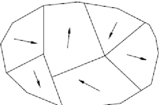
The magnetic materials are represented by various magnetic dipoles and accordingly by numerous magnetic moments. The ferromagnetic materials, as indicated by the solid interaction between the magnetic moments comprise of numerous little volumes, domains even without an external applied field. In Figure 2-2 a domain structure of a ferromagnetic substance is plotted.
Figure 2.2: Domain Structure in a Ferromagnetic Material
The nearness of the domain structures was initially hypothesized by P. Weiss in 1907 by the speculation that the ferromagnetic material is made from numerous regions, domains, every one of them is magnetized to saturation toward some path. The primary exploratory check on the presence of the ferromagnetic domains was selected by Barkhausen in 1919 (George Heinrich Barkhausen, 1881 - 1956).
Barkhausen amplified the voltage beats incited in the secondary coil wounded on a ferromagnetic sample. As the magnetic field was expanded easily a progression of snap was heard. The presence of the characteristic noise demonstrated that the magnetization procedure comprises numerous little irregular flux changes. These discontinuities in the induction can be viewed as abrupt intermittent turn toward the magnetization inside the domains and the irregular movement of the domain boundaries. The two mechanisms happen during the magnetization procedure and they are characterized as Barkhausen noise.
These days a few strategies are produced for perception of the domain structures. Two of them, the Faraday and the Kerr effects are identified with the magneto-optical techniques, in which the axis of the polarization in a linearly polarized light beam is pivoted by the activity of a magnetic field. The phenomenon when in an energized light beam, thought about the outside of a Magnetic material, the bearing of the Polarization is pivoting is known as Kerr impact (John Kerr, 1824 - 1907), while if the turn of the Polarization Axis is started from the transmission of a polarized light bar through a ferromagnetic material is known as Faraday effect (Michael Faraday,1791 - 1867).
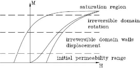
At the point when a magnetic field is applied to a ferromagnetic substance the adjustment in the domain structures, the reversible and irreversible rotation of the magnetic moments inside the domains and the reversible and irreversible movement of the domain walls, relate to the magnetization characteristics. Anyhow, within the magnetization procedure both the reversible and the irreversible changes happen together, four unique ranges on the magnetization characteristic can be recognized by the basically accomplished alters while the domain magnetization and in the intensity of unconstrained magnetization in Figure 2.3.
12
Figure 2.3: Magnetization Mechanism
Beginning from the demagnetized state the principal area on the magnetization characteristic, where the magnetization changes reversibly is the reversible or the starting range. At low field amplitudes the magnetization can be portrayed by the reversible rotation of the domains from a steady state toward the applied field bearing. In this range the reversible magnetization is cultivated by the reversible rotation of the domain walls. Along this area of the magnetization characteristic the initial susceptibility has little values for crystalline substances as , while for
Soft magnetic materials this susceptibility can be found between wide range from
to nearly thousands. The trial information demonstrates that the
Magnetic materials whose crystal structures are less distorted demonstrate less Anisotropy and higher initial susceptibility [5].
2.2 Electromagnetic fields in ferromagnetic materials
The fundamental hypothesis depicting the magnetic field in this part depends on [6]. The magnetic field from a current streaming in a wire can be found by applying Amperes law
H is the magnetic field strength vector, dl is the differential vector from any closed path C. The current enclosed by the path is denoted l. If a coil of wire has N turns equation can be derived from above equation
∗ 𝑙 = 𝐼 ∗ 𝑁 (2.9)
This is the same equation as we have mentioned above mmf.
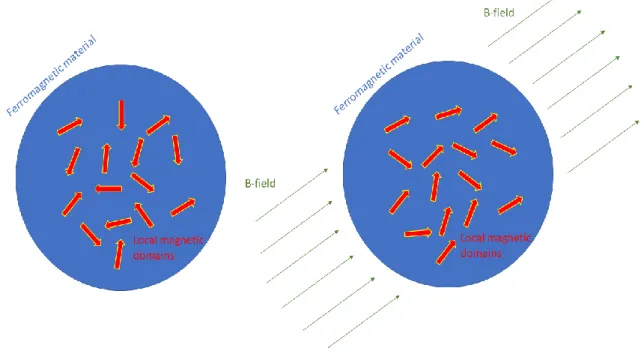
The magnetic domains in materials must be comprehended to foresee how a material reacts to a remotely connected Magnetic Field. All materials comprise little spaces with a little Magnetization. For Unmagnetized materials, the Magnetic orientation is arbitrary in each domain, as can be found in Figure 2.4. The little spaces are represented by bolts and can be viewed as little permanent Magnets. The translation of the Magnetic Domain in a material depends on [7].
14
The domains are exposed to a magnetic field, the impact of the magnetic orientation relies upon the magnetic property of the material. There are five principle classifications of magnetic materials: Ferro-, Para-, Dia-, Ferri and antiferromagnetism. The depictions of the magnetic material classifications depend on [7].
The magnetic domain orientation lines up with the remotely connected field for Para-and ferromagnetic materials. The little Permanent magnets in diamagnetic materials adjusts the other way of the outside Field. For each situation, the new orientation causes another global magnetization of the material relying upon the sort of material and the magnetic field strength. The global magnetization will either decrease or fortify the absolute magnetic Field in the material. This impact is portrayed further in [6] and showed for a ferromagnetic material in Figure2.4. Figure 2.5 outlines that the orientation of the magnetic domains changes when the material is presented to a magnetic field. The field quality variety is of significance when ferromagnetic materials are considered.
Figure 2.5: Magnetization of a Ferromagnetic Material due to an External Field
In above figure it may very well be seen that the orientations of the magnetic domains are transformed from the left to the right figure outline. In antiferromagnetic
materials there is no net unconstrained magnetization, consequently the orientation of the magnetic domains isn't changed when the material is presented to a magnetic field.
Ferrimagnetic materials have material properties like both anti-and ferromagnetic materials. The ferrimagnetic material properties won't be depicted further for what it's worth past the extent of this proposition.
The antiferromagnetic materials have a zero net magnetic moment. In diamagnetic materials, the inside instigated electromagnetic field has a heading inverse to the externally applied field. The inward field is frail and diminishes the net field in the material. The paramagnetic materials have a prompted electromagnetic field a similar way as the connected field and in this manner goes about as a field enhancer. The inside incited fields are frail in both Para-and diamagnetic materials. Most materials are either para-or diamagnetic and the relationship between the H-and B-field can be depicted as around straight in the two cases. The following hypothesis depends on [8] and the relationship is depicted as of now in equation above
= 𝜇 (2.10)
Para-and diamagnetic materials have a low relative permeability (near one). Paramagnetic materials have a relative permeability somewhat higher than one and are pulled in to the magnetic field. The diamagnetic materials have a relative permeability marginally lower than one and are repelled by magnetic fields. As referenced, the para-and diamagnetic materials can be respected as straight materials. Likewise, the conditions are just substantial if the materials are homogeneous furthermore, isotropic. Isotropic materials have a similar material property in every direction. In this case, it implies that a magnetic field can be applied from any course and the material reaction would be equivalent if the geometrical aspect is
16
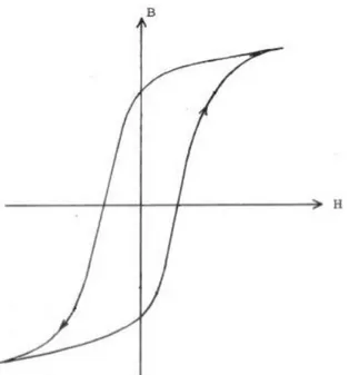
considered, this suggests the little domains will require some opportunity to line up with the applied magnetic field. If the applied field is sinusoidal, the local Induced field is deferred because of the movement. The impact is likewise present when the polarization changes. This marvel makes the all-out field become non-straight and reliant on the applied field. Another imperative marvel is that there is a cutoff to how much the nearby field can expand the all-out field. The magnetic field Strength of the remotely connected magnetic field decides what number of and to which degree the little magnetic domains are influenced. The material ends up saturated when the magnetic domains are lined up with the outside field. An expansion in the magnetic field will not be improved by the material, which means that the behaviour of the material is changed. A further increment of the H-field will just change the B-field as it would in 'free air'. This characteristic conduct results in the hysteresis curve, appearing in figure 2.6.
Figure 2.6: Hysteresis Curve Figure
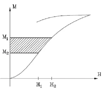
The Ferromagnetic substance can be represented with the energy of the magnetization. If the charge is expanded structure state B1, M1, H1, to B2, M2, H2, under the activity of a magnetic field H, parallel to the magnetization, the work required to magnetize a unit volume can be connected by the relation
∫
(2.11)
So, this energy can be characterized with the area nearby by the ordinate axes M1,
M2 and the magnetization curve as it is plotted in Figure 2.7.
Figure 2.7: The Energy Essential to Magnetize a Unit Volume of the Ferromagnetic Material.
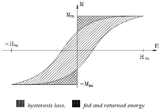
Among one cycle of the hysteresis loops the energy provided by this work is mostly deposited as potential or field energy and furthermore mostly disseminated as heat in the substance. All through one cycle of the hysteresis loops the potential energy should come back to its unique values, with the goal that the resultant work must be consumed as heat. This heat is the hysteresis loss. Proceeding onward the hysteresis loops to the point represented by the magnetized values Hm, Mm, the provided Energy is equivalent to the zone encompassing by the hysteresis curve and the axis M. Along the demagnetizing some portion of the hysteresis curve up to the point of
18
more energy is required. Keep on the process for an absolute cycle of the hysteresis loops the segment of the provided and the returned Energy is plotted in Figure 2.8.
Figure 2.8: Energy State of the Hysteresis Loop
For engineering applications based on the coercive field the ferromagnetic materials can be surrogated soft and hard magnets. Soft magnetic materials are ordinarily utilized for iron cores of transformers, motors and generators and for these reasons‟ high permeability, low coercive field and little hysteresis loss are required. Then again, hard magnetic materials are utilized as permanent magnets in gear for high coercive field, where high remanence and wide hysteresis are appealing. The materials of magnetic recording have the properties like the permanent magnets. They need moderately high remanent induction and adequately high coercivity to avoid the loss of data by the unexpected demagnetization. It is fascinating that the principle uses of the ferromagnetic materials are divided into two fields required practically inverse properties.
2.3 Losses in ferromagnetic materials
The characteristic Hysteresis Loop is a property in ferromagnetic materials. There is a loss in the material when an externally connected field is exposed to the ferromagnetic material. Concurring to [7] it is normally acknowledged to isolate the absolute loss into hysteresis Loss, eddy current Loss furthermore, regularly bizarre losses (otherwise called anomalous losses).
2.4 Hysteresis losses
As depicted above, the magnetic orientation of the domains in the ferromagnetic material changes. This change requires electromagnetic vitality which scatters in the material as heat. The hysteresis loss begins from the adjustment in domain wall motion [6]. Ferromagnetic materials are separated into hard magnetic and soft magnetic materials. Hard magnetic materials require a lot of electromagnetic vitality to move the magnetic domains. This causes a bigger postponement between the adjustment in the externally applied field and the adjustment in the locally induced field. This causes the hysteresis impact. The magnetic domains in soft magnetic materials move quicker, in this manner the magnetic vitality required is fundamentally more in hard magnetic materials.
The magnetizing procedure is portrayed in Figure 2.9. It may very well be seen that the zone limited by the hysteresis Loop shows the energy that scatters as heat in the material. The zone kept by the hysteresis Loop is the distinction between the provided energy to the material and the energy conveyed back to the source. The provided electromagnetic energy amid magnetization of the material is illustrated by the territory a-b-0-d-a. The electromagnetic energy exchanged back to the source amid demagnetization is illustrated by the territory a-b-c-a.
20
Figure 2.9: Energy Degeneracy Due to the Hysteresis
In the figure above, it may be comprehended that during the magnetization of the ferromagnetic material, the material 'expends' electromagnetic energy and during demagnetization the material conveys electromagnetic energy back to the source. The distinction between these amounts is the dispersed energy in the material. This additionally infers that dB is delicate to a negative or positive rate of change.
2.5 MH & BH hysteresis loop
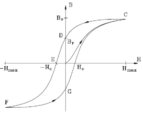
The magnetization procedure is partially irreversible. charging a ferromagnetic material first with dreary expanding field and after reaching the saturation state with a repetitive diminishing field, the magnetization does not return along the first curve, to the equivalent magnetic field has a place diverse estimation of magnetization and magnetic induction. If the magnetic field is diminished from the saturated state, from the point C, the magnetic flux density and the magnetization are slowly diminished along CD as it is plotted in figure[5].
Figure 2.10: Ideal Hysteresis Loop
If the applied field is decreased to zero H = 0, in the point D the appearance demonstrates retentivity. As per the irreversibility of the procedure the magnetization and the magnetic Induction have limited values, the remaining, or the remanent magnetization and induction individually Mr = Br / μ0. Further reducing the magnetic
Field, it turns to negative esteem, coming about a continuous reduction in the magnetization. The estimation of the magnetic field at point E is the coercive field Hc, B = 0. The DE segment of the curve is indicated as demagnetizing curve, where
an inverse coordinated field needs to apply to lessen the magnetic induction to zero. At point E the magnetization M has a limited value as indicated by the relation μ0 (H
+ M) = 0, as it is plotted in Figure 2-10. Further increment of the magnetic field H, in negative sense, until the point F, results an increment of the magnetic flux density and of the magnetization, at last it prompts a negative saturation. if the field is turned around in positive sense, the magnetization will change, lastly shut along FGC. The closed loop CDEFGC of the B - H curve or the equal M - H curve is the Hysteresis
22
Figure 2.11: Stabilization of the Loop
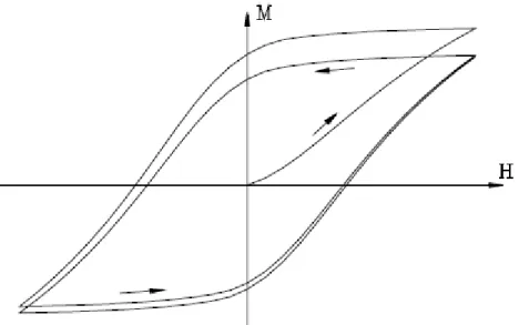
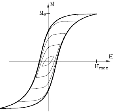
Through a gradually changing cyclic magnetization process the rotation of the magnetic field between similar qualities results a balanced out unfaltering hysteresis Loop of the magnetization. The experimental information demonstrates 8 -10 cycles before adjustment of the magnetization process. The adjustment of the hysteresis loop is portrayed by the repetitive diminishing additions in the remanent magnetization among the magnetization cycles. The adjustment of the hysteresis can be quickened by the utilization of higher field in the magnetization procedure. The higher abundancy of the excitation field results in more extensive Hysteresis with distinctive shapes as it tends to be found in Figure 2.12.
Figure 2.12: Different Serial of Hysteresis Loops
There are endless number of hysteresis loops having a place with various most extreme estimation of the excitation. As the underlying positive field is expanded, the region of the associated hysteresis loop rises lastly approaches roughly to a maximum, where the Loops are corresponded and closed before the highest field is revive. The hysteresis loop having a place with the foremost region is the major Hysteresis loop, or the hysteresis attractor.
The Magnetic properties of various materials can be represented with the curve of the tip points characterized by the balanced-out Hysteresis Loops at various amplitudes of varying fields. This curve is the fundamental magnetization curve or the commutation curve. The upper portion of the symmetrical Hysteresis Loops with the commutation curve is plotted in Figure 2.13.
24
Figure 2.13: Fundamental Magnetization Curve of Hysteresis Loop A few cases rather than the Magnetic Susceptibility the Magnetic Permeability are used to with represent the connection between the applied magnetic field intensity H and the magnetic induction B.
2.6 Eddy current losses
The established losses comprise of the ohmic Losses (in a current carrying conductor) and the eddy current losses. The eddy current is a result of the materials reluctance to magnetize. At the point when the conductive material is presented to a rotating electromagnetic field the material will act against the external field by creating a nearby counter field. This impact is delineated in Figure 2.14.
Figure 2.14: Induced Eddy Currents and Magnetic Counter Field
The basic segment of a turning or static electrical machine is its magnetic core amassed from a suitable magnetically hard (permanent) or soft magnetic material. The magnetic core is intended to intensify, control the bearing of the magnetic flux that thusly decides a machine's act whether it is a transformer, motor, generator, or other electromagnetic gadget. Contingent upon the machine type and design, the core may be polarized by a steady (DC) magnetic field or an alternating (AC) field. At the point when an AC magnetic field is connected, magnetization happens as the material is consistently charged by inside rearrangement of magnetic domains in complex procedures that reason eddy currents to stream in the material. These eddy
26
because of local overheating or thermal cycling [8]. Second, magnetic core loss represents an immense measure of squander Energy all through the world. For instance, although extensive power transformers can be over 98% productive, the cost of the losses over a machine's lifetime can far surpass its capital expense.
2.7 Hysteresis Models
Hysteresis curves for core materials that have been used in power electronics and applications for decades, broadly fluctuated. Moreover, action into saturation through and throughout predispositions is conceivable over temperature and frequency range. These mechanisms consolidate to make a definite picture very unpredictable.
The best possible choice of a magnetic material model includes various thoughts which can be inexactly gathered into different classifications: corporal in addition cost. Physical contemplations incorporate limit of model to depict the material in satisfactory detail and to the mandatory precision over the working limits of intrigue. These necessities are basically end-client configuration subordinate. Rate contemplations tell about the model is to be used, initially by the test system creator after that by the end-client. In this manner, in context on the unpredictability of the adjustments to be settled on in model decision, not one model will be all generally satisfactory.
2.8 Modeling Magnetic Materials
Materials for magnetic cores are very complex and their properties and what happening in the material is not completely understood. No complete model exists as of now and the modeling methodologies till now a day drop into two general groups: theoretical and empirical. The theoretical models attempt to statistically show total impacts of experiential or speculated physical phenomena. All depend on physical test data for evaluation parameters. Most of them were advanced a sort of physical or application, and henceforth, may introduce challenges when functional in general. The empirical-models are partitioned into two classifications: function-fitting and conceptual. In case of the empirical function-fitting a function is picked parameters are altered in accordance as per suitable the information. Structure directive of the function (or equation) is assured, along these lines, any needed suitable can be
cultivated by the expense of multifaceted nature. In empirical-model data is commonly defined by a low order differential equation or on the other hand by the solution for the equivalent. As of they are not high order, the models have upside of an attentively direct physical comprehension. This understanding essential not be exact to be valued to a user end. The difference among the two observational cases is fundamentally a matter of finding with respect to the authors.
Hybrid models suitable for many classes. Methodology is regularly taken into account when a specific phenomenon is surely known furthermore, can be depicted hypothetically yet others requirement be demonstrated empirically. Additional hybrid case is the opinion at which the material has a generally straightforward conduct yet to accomplish the required exactness the model must fuse complex sub components. In this thesis hybrids are not independently classified, rather, such models are assembled into what is decided to be the dominant classification.
The mathematical explanation utilized in models in all classifications was cultivated in either (or now and again both) of dual unmistakable customs. Single strategy remained a plan utilizing ordinary equation. These commonly are then statistically executed utilizing a general software design language, a mathematical calculation bundle or a simple HDL. The substitute technique is to make as a full-scale model. It is a portrayal of a differential condition through an identical system for electrical components. Model is at that point arithmetically actualized utilizing a circuit test system. The Models composed utilizing a simple HDL are quicker and progressively adaptable than large scale models; nonetheless, full scale models are favored for test systems without simple HDL ability[9].The associated subsections plan a portion of the current models in every one of the classes.
2.9 Theoretical
The fundamental systems of magnetization are domain wall movement and domain rotation. The wall movement has revocable and permanent segments. There are a few models which regularly portray just piece of these instruments. Jiles and Atherton
28 2.10 Empirical-conceptual
A resemblance between models in this class is one of nonlinear functions in differential equation is anhysteretic curve and a function direct recognized with model. Subsequently, it might be anticipated that by choosing of this function decides the materials the model defines finest.
Table 2.1: Theoretical Models Author Model S.H.Charap 1974 [8] 𝑁 𝑁 𝑁 𝑁 𝑙 Magnetic hysteresis model
Tuohv and Panek 1978 [12] 𝜇 𝜇 | | Chopping of transformer magnetizing currents Jiles&Atherton1986-1993 [10][13][14][15][16] ( ( ) ( )) a, c, k, a are coefficients is 1 or -1 dependent on the dH/dt;
M = Magnetization; Ms = Saturation magnetization
Stoner and Wohlfarth [11] (1948)
Domain rotation as the main mechanism of hysteresis.
Preisach (1935-1993)
∬ .
3. Fe-Sn-B ALLOY AND JA MODEL 3.1 Fe-Sn-B Amorphous Alloy System
The well-known traditional rapidly quenched nanocrystalline soft magnetic materials for example FINEMET, NANOPERM and HITPERM are currently upheld by new intensely examined systems. Amongst these a special consideration is put on materials with high saturation magnetization whereas preserving low coercivity. Diverse systems based on Fe-B with accompaniments of Co, Cu, C, P, Si and other elements were developed, which achieve necessities on current soft magnetic materials. Recently a new system of nanocrystalline soft magnetic alloys based on Fe-Sn-B has been anticipated, where the effect due to the presence of Nb or Zr, specifically nanograin size control, is attained by adding of Sn into Fe-rich Fe-B system.
Additional investigation of rapidly quenched Fe-Sn-B system has directed to partial replacement of B and Fe by Si and to doping of the base alloy with slight amounts of Cu. Ribbons with changing Si content were set by planar flow casting, directing the foundation of fine-grained structure after controlled annealing. The effects of the replacements and of doping with Cu on stability, Nano crystallization process, subsequent magnetic properties and structure of the moulded phases were studied by thermogravimetry, vibrating sample magnetometry, differential scanning calorimetry, conventional and in-situ x-ray diffraction and transmission electron microscopy. The results will be associated to the performance and structure of the classical nanocrystal-forming systems and the application potential of the new system as soft magnetic material will be evaluated.
The amorphous alloys have many bases, Fe-B based alloys are the superlative representatives of the traditional metallic glass systems which have many applications according to the soft magnetic features. They have been a extensive
32
amorphous alloys which was associated to Fe-Si-B systems. Those stages have importance in considerate the soft magnetic materials behaviours. The effects of addition numerous elements can be found in literature nonetheless a few results have been issued for rapidly quenched Fe-Sn-B ribbons for the fact that Sn element just liquifies in the solid Fe (Sn) and formulae no solid dispersion with B. This can be under the statement of negatively affect glass forming aptitude of any Fe-Sn-B alloy. However, the effect of adding Sn can be examined by numerous reasons for example atomic radius misfit, low melting temperature and representing a Mössbauer active element applying the method for microstructural analysis.
The different rapidly quenched compositions of Fe-Sn-Si-B were examined by means of the microstructure and morphology of the phases formed upon thermally activated crystallization. The quantities were taken from X-ray diffraction, transmission electron microscopy and differential scanning calorimetry.
3.2 Experimental Details
Amorphous ribbons with thinness around 20-30µm and width of 6 mm were prepared by planar flow casting from master alloys with variable chemical compositions (purity of the components was better than 99.9%). Casting of ribbons performed after induction melting of the master alloys to casting temperatures about 200 K higher than the alloy melting point. The planar flow casting temperature was from 1200°C to 1250°C variably and for all the samples there was a waiting time for 1 min at 1100°C before heating to the final casting temperature. The composition of the prepared samples with the results from differential scanning calorimetry are in Table 1. The amorphous state after rapid quenching was checked by X-ray diffraction analysis (XRD) in Bragg–Brentano geometry using Bruker D8 Advance diffractometer (Cu Kα radiation).
Samples were polished by ion-beam milling using aGatan PIPS machine. The microstructure and morphology of the crystallized products were analysed by transmission electron microscopy (TEM) using conventional JEOL JEM-2000FX electron microscope.
Ribbons were weighed and prepared for the thermal measurements in differential scanning calorimetry (DSC)(Perkin–ElmerDSC7). The programme was
given in five steps. First step was heating from 40°C-600°C, heating rate 10°C/min. Then cooling from 600°C-40°C at heating rate of 40°C /min. Hold for 5 minutes at 40 °C for stabilization. Then the first and the second steps were repeated respectively to obtain the proper baseline-subtracted DSC signal.
Results from thermal analysis of differential scanning calorimetry (DSC): the temperature of the crystallizations onset Tx, the temperature of the maximum
crystallizations rate Tmax.
Table 3.1: Temperatures Composition Tx1(K) ±0.2 Tmax1(K) ±0.2 Tx2(K) ±0.2 Tmax2(K) ±0.2 Fe81Sn7Si2B10 379,15°C 395,60°C 504,19°C 511,36°C Fe81Sn7Si2B10 379,79°C 397,26°C 521,42°C 527,72°C Fe81Sn7Si5B7 371,84°C 385,51°C 518,84°C 526,06°C Fe83Sn5Si2B10 370,32°C 394,43°C 501,99°C 507,71°C Fe83Sn5Si5B7 332,75°C 368,27°C 516,41°C 522,58°C Fe83Sn5Si2B10 371,21°C 393,45°C 502,06°C 507,72°C
There are three constituting binaries in the Fe–Si–Sn ternary system, Fe–Si, Fe–Sn and Si–Sn systems. The Fe–Si binary system thermodynamically assessed by Lacaze and Sundman has been widely accepted in literature .There are five intermetallic compounds in the Fe–Si binary system: Fe2Si, Fe5Si3, FeSi, FeSi2–H and FeSi2–L. The solution phases are: liquid, (γ–Fe) and (α–Fe). In addition, the Bcc–solid solution has two existence forms, disordered α–Fe (A2) and ordered α1 (B2) and α2 (D03).
The equilibrium phase diagram of the Fe–Sn system has been investigated intensively by many authors.s Thermodynamic descriptions developed by Nüssler et al. included two metastable phases Fe3Sn and Fe0.565Sn0.435, while the stable
34
and FeSn2. The liquid phase encompasses a miscibility gap within the composition between 31.2 at% Si and 81.1 at% Si. Fe5Sn3 is stable between 773.4 °C and 901.1 °C. The Fe3Sn2 phase is formed by a peritectic reaction at801.8 °C, and it transforms into the (α–Fe) and Fe-Sn phases by a eutectoid reaction at 601.9 °C. The Fe-Sn and FeSn2 phases are the products of another two peritectic reactions reacted at 751.7 °C and 502.4 °C, respectively. The Si–Sn binary system contains a eutectic reaction at 231.9 °C. The eutectic point is very close to the melting point of pure Sn. Under normal pressure, the stable phases are: liquid, the (Si) solid solution and the (Sn) solid solution. No binary compound exists in this system. More information about the crystal structure of phases in above three binary systems is shown in Table 1. No ternary compound was reported from the available literature. Among the above three binary systems, only the Fe–Sn system has the miscibility gap characterizing formation of the immiscible alloy, so much attention should be paid to the role of Si on the solidification of Fe–Sn based alloy. In this work, phase relationship between Fe–Sn compounds and Fe–Si compounds was investigated by constructing isothermal sections of the Fe–Si–Sn systems at 700 °C and 890 °C. Vertical section of this system was established to analyse the solidification process.
3.3 Langevin theory for parameters
Langevin hypothetical that in paramagnetic material the moments are not interacting, so the traditional Boltzmann measurement can be used to direct the probability of any given electron inhabiting an energy state of Wm
(3.1)
The equation relating the magnetization for paramagnetic materials in respect of magnetic momemts aligned analogous to the applied field can be related as:
𝑁 (3.2)
Here,
𝜇
The function in the digression is called Langevin function:
⁄
The range of the function lies between -1< <1. for the maximum values for the parameter , the Langevin function must be 1. As the lim H approaches to infinity (∞) the magnetization must be 𝑁 The moments incline to be seamlessly aligned. As we can see in the expression , saturation occurs only when, the external filed is very high and the temperature should be extremely low. In the practical the magnitude of is small at room temperature. For any given data the relation given above results as small values as for .
For the small values of the series expansion results magnetization M, and field independent susceptibility, ᵪ
𝜇
(3.3)
The Langevin model principals the known Curie law for para-magnetics susceptibility. The hysteresis free magnetization features can be determined by the equation:
(3.4)
For,
Ms = 1.7 * 106 A/m
a = 800 A/m
36
Figure 3.1: Hysteresis free Langevin Magnetization Curve
As Weiss law the magnetization characteristics resulted by Langevin theory, mentioned above in equation (3.2), has been modified and published for ferromagnetic materials by Jiles [20].
* 𝜇
𝜇 +
(3.5)
For isotropic materials, due to the interaction the magnetization characteristics described by the relation:
[
]
3.4 Jiles Atherton model
Jiles-Atherton theory of ferromagnetic hysteresis [10] is extensively used for the modeling of soft magnetic materials. Over 30 years, the J-A model advanced into different versions. In this section we will list the classic A model and correction J-A model mathematically and after that we will simulate these models for our Fe-Sn-B Amorphous material in MATLAFe-Sn-B Simulink environment.
3.4.1 Classic J-A Model
In 1984, Dr. Jiles and Dr. Atherton first predicted by means of a changed Langevin function to derive an anhysteretic magnetization curve[21]
( ) (3.7)
Here,
⁄ (3.8)
𝜇 (3.9)
H - Magnetic field intensity; M - Magnetic moment;
m - Magnetic moment per unit volume; - Boltzmann‟s constant;
T - Temperature in Kelvin; 𝜇 - permeability of free space
The first publication of J-A method is complex, and computation is awkward. In later publications, the authors lead up to two components- the irreversible magnetization component and the reversible component to represent M,
38
By this method, the J-A model is easy to calculate. An altered mathematic method is given by the authors to shorten the anhysteretic magnetization equation.
(3.11)
Where Ms is the core material saturation magnetic moment. To generate the arbitrary
function ƒ(He), a Langevin equation is chosen to model.
⁄ (3.12)
The Man is derived
[ ] (3.13)
a is used to describe the sharp of Man
(3.14)
. is the domain coupling.
In the 1986 paper, the irreversible component of magnetization is given,
𝜇⁄
(3.15)
And the reversible component is described as,
(3.16)
(3.17) (3.18) And, (3.19)
Now put the values of reversible and irreversible components that yields, 𝜇⁄ (3.20) 𝜇⁄ (3.21) 𝜇⁄ (3.22) 𝜇⁄ (3.23) 𝜇⁄ (3.24)
assurances that incremental susceptibility will be positive. 3.4.2 Modified J-A Model
40
(3.25)
The reversible component can be represented as the difference between the anhysteric and irreversible magnetization.
(3.26)
The energy balance in the change of the supplied energy, the magnetic energy and the hysteresis loss generated by domain wall motion can be expressed, [ref of the hysteresis modeling]
𝜇 ∫ 𝜇 ∫ 𝜇 ∫
(3.27)
By differentiating above equation, it results in the relation between the magnetic field intensity and magnetization,
(3.28)
Where means domain pinning parameter.
Considering the interaction between the domain according to Weiss law, with effective field,
(3.29)
The reversible magnetization is given with,
(3.30) (3.31) (3.32) By combining we get,
(3.33)
The JA model have multiple versions and do not has a unique expression. The readers may find difficulties to comprehend the theory. These troubles indicate the accuracy when analyzing the JA theory. Many authors make queries from the formula of anhysteretic magnetization curve and the derivation of energy loss equation.
One of them is about anhysteretic magnetization. We know an anhysteretic curve is produced by the contact of external magnetic field and magnetic domain, and the expression is described equation (3.11). the classical JA model describes Man into
two different forms, according to equation (3.13),
In the equation (3.29) the effective field He is described as,
And the other one is described in references also, but in this equation the magnetization in effective field is anhysteretic magnetization,
(3.34)
The derivation we did above for the total magnetization Man ≠ M, so we must
determine in our model which Man should be used. According to equation (3.12) the
42
Figure 3.2: Langevin Diagram
The appropriate expression for Man should be according to equation (3.34).
The second thing is the process of derivation of M, the references does not explain. We already explained above that total magnetization of a material is equal to the summation of irreversible and reversible magnetization equation (5.4),
The reversible magnetization is according to equation,
The energy associated by magnetization M might well-thought-out as the change among lossless and losses because of the hysteresis, the equation described below id stated in [10]:
𝜇 ∫
𝜇 ∫ 𝜇 ∫
(3.35)
By differentiation above equation (3.35) we get:
(3.36)
Now, from equation (5.4) and equation (5.10) we will calculate the irreversible magnetization ( ):
(3.37)
The effective magnetization according to the equation (5.24):
By differentiating the above, we get
(3.38)
Substitute equation (3.36) by equations (3.37) and (3.38), we get a differential equation for hysteresis according to the JA model:
(3.39)
Man, expression should be according to equation (3.34). The equation (3.39) is
4. RESULTS AND DISCUSIIONS
4.1 Implementation of J-A Model in MATLAB
In this section, we will explain how we will program and model the JA hysteresis model in MATLAB and Simulink. There are many types of JA models, we will develop classical JA model and Modified JA model. First, we will compare the results of classical and modified JA model by using the initial values for JA parameters described in his publications.
For different samples the hysteresis is different. For modeling the hysteresis, we need to find the parameters first. Five variables are needed, Ms, a, k, c and α. These
parameters can be obtained by the following equations[13].
(4.1) (4.2) (4.3)
is the initial normal susceptibility, is the initial anhysteric susceptibility,
is the differential value of maximum susceptibility. The saturation magnetization (Ms) is obtained from the material data sheet.
We have constructed a model based on the equation (3.39) in MATLAB Simulink environment. We are unable to acquire the parameters for our material, but we have
46 Table 4.1: Parameters for JA Hysteresis Modeling
Parameters Values a 2000 A/m c 0.1 k 2000 Ms 1.5*106 A/m 0.003
Table 4.2: Parameters for JA Hysteresis Modeling
Parameters Values a 2000 A/m c 0.1 k 4000 Ms 1.5*106 A/m 0.003
The parameters Ms, a, and are given by anhysteric magnetization and they can
identify by the equation 5.7. the other parameters have some ranges based on the coercive field (Hc), for the differential evolution-based optimization parameter Ms is in the range of Bmax/ and 2Bmax/ . And the parameter a should be in the range of 0.2Hc and 5Hc. the identified parameter k has the values in the range 0.2Hc and 5Hc. parameter c is in the range of 10-6 to 1. We have already discussed that we were unable to find our parameters for our specific material we will do that in our future work. But here are some exemplary values of parameters we have mentioned above with the reference.
Fist we programmed and modeled the JA expression now we will compare the both classic and revised model equation for the data given in Table 4.1 and 4.2. for a magnetic core we have to set some additional parameters. Based on the following equations, 𝐼 𝑁 ∗ (4.4) ∗ (4.5) (4.6)
Where N is the turn ratio, Lp is the length of the average magnetic path and S is the
cross area of the core. Then a simulation test of the current transformer will be conducted with analog input signal of H to simulate a 1200:5 CT. The amplitude of H will affect hysteresis and determine the saturation degree [22].
48 Table 4.3: Core Parameters
Parameters Values Lp 1.00076 S (m2) 1.5×10⁻³ μ0 (H/m) 4π×10-7 Burden R(Ω) 1 N 240
In the simulation test we used H 20000*(sin (2*pi*f*T)), so we can get a steady state hysteresis curve for any magnetic material. By using the data in table 4.1 we have simulation results for both classic and revised JA model and the difference can be seen clearly.
50
Figure 4.3: Modified JA B-H Hysteresis Loop for Table 4.1