REPUBLIC OF TURKEY SİİRT UNIVERSITY
GRADUATE SCHOOL OF NATURAL AND APPLIED SCIENCES
FACE RECOGNITION USING LBP, nLBP and αLBP ALGORITHMS
MASTER DEGREE THESIS
MEGIR MOHAMMED RASOOL RASOOL
163111014
Department of Electrical and Electronics Engineering
Supervisor: Assist. Prof. Dr. Volkan Müjdat TİRYAKİ
JULY - 2019 SİİRT
v TABLE OF CONTENTS
THESIS NOTIFICATION ... ii
ACKNOWLEDGEMENTS ... Hata! Yer işareti tanımlanmamış. ABBREVIATIONS AND SYMBOL LISTS ... ix
Symbol Description ... x
ÖZET ... xi
ABSTRACT ... xii
1. INTRODUCTION ... 1
1.1. Background ... 1
1.1.1. Why Face Recognition? ... 1
1.2. History of Face Recognition ... 2
1.3. Face Recognition ... 3
1.4. Local Binary Pattern (LBP) ... 4
1.5 Why is LBP used in face recognition? ... 4
1.6 Applying LBP in Facial Recognition ... 4
1.7 Advantages of LBP ... 4
1.8 Problem Statement ... 4
2. LITERATURE REVIEW ... 6
2.1 Historical Background ... 6
2.2 Time Evolution and Modern Techniques ... 6
2.3 Face Detection ... 6
2.4 Face Recognition ... 7
2.5 Application of LBP Texture Features in Face Recognition ... 7
2.6 Multi-scale LBP Histograms for Facial Recognition ... 8
2.7 An Extensive Approach to Near Infrared Face Recognition Grounded On ELBP ... 8
2.8 Multi-scale Block LBP for Face Recognition ... 8
2.9 Local Gabor Binary Pattern Histogram Sequence (LGBPHS) for Face Representation and Recognition ... 9
3. MATERIALS AND METHODS ... 10
3.1. Materials ... 10
3.2. Methods... 11
3.2.1.Conventional Local Binary Pattern Operator ... 11
3.2.2. Local binary patterns based on relations between neighbors: neighborliness LBP ... 13
3.2.3. Local Binary Patterns based on angles : αLBP ... 15
3.3. Proposed Face Recognition System ... 17
3.3.1. Classification Methods ... 17
3.3.1.1. Artificial Neural Networks (ANN) ... 17
3.3.1.2. kNN Method ... 18
3.4. kNN algorithm steps ... 19
vi
3.4.2. K number and its effect on classification ... 20
3.4.3. Cross validity test ... 21
3.4.5. Performance Measures ... 22 3.6. Accuracy ... 22 3.7. Error rate ... 22 3.8. Precision ... 23 3.8.1. Recall ... 23 3.8.2. F-measure ... 23 4. RESULTS ... 24
4.1. Results for nLBP (neighborliness Local Binary Pattern) ... 24
4.2. Results for αLBP ... 27
4.3. Results for Classic LBP ... 30
4.5. Comparison of Models ... 32
4.6. Comparison of Different Machine Learning Methods ... 32
4.7. Comparison with the Studies in Literature... 33
SRC, sparse representation based classification ... 33
Extended SRC ... 33
5. CONCLUSION ... 34
REFERENCES ... 36
vii
LIST OF FIGURES
Figure 3. 1. Sample images in ORL database ... 10
Figure 3. 2. Cropped images of sample images ... 11
Figure 3. 3.Calculatingthe original LBP code... 12
Figure 3. 4. Circularlysymmetricneighborsets for different LBP operators. ... 13
Figure 3. 5. Overview of the first proposed method. Relations between neighbor based LBP ... 13
Figure 3. 6. Overview of the second proposed method. Angles based LBP(αLBP) ... 15
Figure 3. 7. Proposed Face Detection System ... 17
Figure 3. 8. A simple ANN architecture. ... 18
Figure 4. 1. Formed faces according to different d values with nLBP method. ... 24
Figure 4. 2. nLBP method histograms of faces formed by different values of parameter d ... 25
Figure 4. 3. Achievement results according to different distance (d) values ... 26
Figure 4. 4. faces formed by the αLBP method according to different α values. ... 27
Figure 4. 5. αLBP method histograms of faces formed by different values of α parameter ... 28
Figure 4. 6. Success rates according to different angle values ... 29
Figure 4. 7. LBP faces ... 30
viii
LIST OF TABLES
Table 3. 1. Performance criteria ... 22
Table 4. 1. Results obtained with kNN and ANN for nLBP ... 25
Table 4. 2. Performance measures obtained with kNN for nLBP features ... 26
Table 4. 3. nLBP for performance measures ... 27
Table 4. 4. Success rates with kNN and ANN classification methods for αLBP features29 Table 4. 5. Performance measures obtained with kNN for αLBP ... 30
Table 4. 6. Performance measures obtained with ANN for αLBP ... 30
Table 4. 7. Performance measures obtained with kNN and ANN for LBP ... 31
Table 4. 8. Comparison of methods ... 32
Table 4. 9. Performance measures obtained by different machine learning methods .... 33
ix
ABBREVIATIONS AND SYMBOL LISTS
Abbreviation Explanation
2DPCA : Two-dimensional Principal Component Analysis
αLBP : angle based local binary pattern
ANN : Artificial Neural Network
CLBP : accomplished LBP
CLBP_M : components: CLBP-Magnitude
DT-LBP : dataset test LBP
EER : Equal Error Rate
ELBP : Extended Local Binary Pattern
ESKPCA : improved by sparse Kernel Principal Component Analysis
kNN : k-nearest neighbors
KPCA : Kernel Principal Component Analysis
LBP : Local binary pattern
LDA : Linear discriminant analysis
LGBPHS : Local Gabor Binary Pattern Histogram Sequence
LRC : Linear Regression Classification
MB-LBP : Multi-scale Block Local Binary Pattern
nLBP : Neighborliness local binary pattern
PCA : Principal Component Analysis
PGM : Portable Gray Map
PIN : Personal Identification Number ROC : Receiver Operating Characteristic SRC : Sparse Representation based Classifier
SVM : Support Vector Machine
ULBP : Uniform local binary pattern
x
Symbol Description
: pixels around the center Pixel : center Pixel
: comparison function
P : pixels around the center Pixel d: distance α : Angle values : output of ANN : inputs of ANN : weights in ANN test sample in kNN normalized values
: original values in dataset for kNN K: number of neighbors in kNN cross validation test
TN: True Negative TP: True Positive FN: False Negative FP: False Positive
xi
ÖZET
YÜKSEK LİSANS TEZİ
LBP, nLBP ve αLBP ALGORİTMALARI KULLANILARAK YÜZ TANIMA
M.Sc.Thesis
Megir Mohammad Rasool RASOOL Siirt Üniversitesi Fen Bilimleri Enstitüsü Danışman: Dr. Öğr. Üyesi Volkan Müjdat TİRYAKİ
Temmuz 2019, 40 sayfa
Yüz tanıma, son yıllarda en önemli görüntü işleme uygulamalarından biri olarak büyük ilgi görmektedir. Yüz tanıma problemi için yapılan çalışmalara bakıldığında başarı oranları yüksek olmasına rağmen kontrolsüz ortamlardaki performans henüz insanlardan daha iyi değildir. Kısıtlı olmayan ortamlarda, bilgisayar görüsü ve örüntü tanıma konusunda doğru ve kararlı yüz tanıma ile ilgili birçok zorluk vardır. Bu tez çalışmasında yüz tanıma problemi için klasik LBP, nLBP ve αLBP kullanılmıştır. nLBP piksellerin komşuları arasındaki ilişkiye göre oluşturulmaktadır. nLBP‟nin d uzaklığına bağlı bir parametresi bulunmaktadır. Bu parametre karşılaştırılacak ardışık komşular arasındaki mesafeyi belirtir. Farklı d parametre değerleri için farklı örüntüler elde edilmektedir. αLBP operatörü ise her pikselin değerini bir açı değerine göre hesaplamaktadır. Açı değerleri α=0, 45, 90 ve 135 derecelerinden biri olmaktadır. Önerilen yaklaşımları test etmek için ORL yüz veri tabanı kullanılmıştır. ORL yüz görüntülerinden nLBP, αLBP ve klasik LBP ile elde edilen öznitelikler kNN ve ANN makine öğrenmesi yöntemleri kullanılarak sınıflandırma işlemleri gerçekleştirilmiştir. nLBP öznitelikleri ile kNN kullanılarak en yüksek %98.25 başarı oranı gözlenmiştir. αLBP öznitelikleri ile ANN kullanılarak %88.50 başarı oranı elde edilmiştir. Klasik LBP öznitelikler ile ise en yüksek %83.50 başarı oranı elde edilmiştir. Önerilen nLBP ve αLBP yaklaşımların klasik LBP yönteminden daha başarılı olduğu görülmüştür. Yapılan literatür çalışmasında aynı ORL yüz veritabanı üzerinde yapılan çalışmalarda elde edilen başarı oranları bu tez çalışmasında önerilen yaklaşımların başarı oranları ile karşılaştırılmıştır. Sonuç olarak önerilen LBP tabanlı yaklaşımlar kullanılarak yüz tanımada önemli derecede başarı sağlanmıştır.
xii
ABSTRACT
M.Sc. Thesis
FACE RECOGNITION USING LBP, nLBP and αLBP ALGORITHMS MEGIR MOHAMMED RASOOL RASOOL
The Graduate School of Natural and Applied Science of Siirt University The Degree of Master of Science
In Electrical-Electronics Engineering
Supervisor: Assist. Prof. Dr. Volkan Müjdat TİRYAKİ
July 2019, 40 pages
Face recognition is of great interest because it is one of the most important image processing applications. Although the success rates of the studies in the literature are high, the performance in out-of-control situations is still not better than human. There are many challenges to design an accurate and robust face recognition system, especially in non-restricted environments. In this thesis classical local binary pattern (LBP), neighborliness local binary pattern (nLBP) and αLBP were used for a face recognition problem. nLBP is formed according to the relationship between the neighbors around each pixel. nLBP has a distance parameter which specifies the distance between consecutive neighbors to be compared. Different patterns are obtained for different d parameter values. αLBP operator calculates the value of each pixel according to an angle value. Angle values can be α = 0, 45, 90 and 135 degrees. The ORL face database was used to test the proposed approaches. nLBP, αLBP and classical LBP features were extracted from face images and classified using k-nearest neighbor (kNN) and artificial neural network (ANN). 98.25% recognition rate was obtained using kNN with nLBP. A recognition rate of 88.50% was obtained with αLBP using ANN. The recognition rate of 83.50% was obtained with classical LBP. The proposed nLBP and αLBP approaches were found to be more successful than the classical LBP method. In the literature, the success rates obtained in the studies performed on the same ORL face database were compared with the success rates of the proposed approaches in this thesis study. As a result, the proposed LBP-based approaches achieved significant success in face recognition.
1 1. INTRODUCTION
Face recognition is a research area encompassing various fields such as physics, mathematics, physiology, biology, computer science as well as others. This study addresses one of the central challenges in face recognition by reviewing several thought-provoking applications and analyzing how effectiveness and efficiency can be improved in the research area with particular focus on the local binary patterns (LBP). For training and testing purposes the ORL face database was used (Samaria and Harter, 1994).
1.1. Background
Woody Bledsoe, Helen Chan Wolf, and Charles Bisson proposed the first facial recognition system in the 1960‟s (Bledsoe 1966a; Bledsoe 1966b). An administrator was needed in the programs to locate the facial features on the photograph. The programs recognized faces by calculating lengths and proportions in relation to certain locus positions which were then equated with known data. Face recognition is a subset of a larger spectrum of pattern recognition technology that is employed in a wide range of activities in life. Facial recognition in natural situations entails the robust performance of three visual tasks: acquisition, normalization and recognition. Acquisition refers to the process by which face-like image patches are recognized and tracked in a dynamic scene. Normalization is the process by which face images are subdivided, oriented and normalized whereas recognition is the process by which they are represented and modeled as individualities, together with the linking of original face images with identified reproductions.
1.1.1. Why Face Recognition?
Due to the increased need for verification of peoples‟ identity, there is the question about which technology is best placed to supply the needed information. There are currently various identification technologies: a good number of these processes have been in actual use for years. Personal Identification Number (PIN) is the most widespread method for verification of personal identity. However, the technique is riddled with several challenges: for instance, it is likely for one to forget or misplace the PIN or perhaps someone may steal it. One effective way of countering such liabilities is through the use of biometric identification systems which employ pattern recognition techniques to recognize the particular characteristics of individuals. Examples of
2
biometric identification systems include fingerprints, retina, and iris recognition. However, some of these biometric techniques are not easy to employ as the user must position himself/herself relative to the sensor and take some time in the identification process although several modern face recognition methods do not require specific positioning.
While the identification process is important in high-security measures, it is not convenient in certain settings such as in a store. The use of video and voice recognition technologies are going to be widespread in the upcoming generations of smart environments. These recognition technologies are usually passive, do not restrain the movement of the user, and are economical. People are more likely to be comfortable using a process that involves face and voice recognition since humans naturally identify one another by their voice and face.
1.2. History of Face Recognition
The practical importance of facial recognition as well as the theoretical interest from cognitive science has made the research area to be as deep-rooted as computer vision. Facial recognition was the result of the increased ability of machines to take up complicated roles as well as possessing the ability to fill in, correct or aid human abilities and senses. Machines have a wider scope for recognition purposes besides facial recognition and can employ such tools as fingerprints or iris scans. Even though biometric methods of identification are more precise, facial recognition has been the subject of focus by various research owing to its non-invasive nature and the fact that it is the most preferred method of person identification by humans. There have been two main methods in the research areas since the onset of person identification technology: geometrical and pictorial approach. The geometrical approach employs the spatial outline of one‟s face. This method first locates the primary geometrical facial features before classifying a person‟s appearance depending on the differing geometrical lengths and slants between the parts of the face. Pictorial approach, in contrast, employs the templates of parts of one‟s face to recognize anterior views of the face. A majority of techniques that employed both approaches share extensions that handle varying poses backgrounds. In addition to the geometric and pictorial methods there is the primary component study method which can be interpreted as a sub-ideal model method together with other recent template-based approaches which are founded on image gradient. There is also the deformable model technique which entails features of both
3
the pictorial and geometry methods and suitable for faces in varying postures or expressions.
1.3. Face Recognition
Facial recognition is a technique of identifying an individual by using a digital image or a video as an input. Facial recognition systems are primarily used as a security measure although they are progressively being employed in several other fields. Contemporary facial recognition methods use faceprints: numeric codes capable of categorizing as many as 80 nodal features on a person‟s face. Nodal features serve as end points that assist in determining the variables of one‟s face like the dimensions of the nose, the profundity of the eye sockets, or the protrusion of the cheekbones. The systems first capture the nodal features on a digital model of a person‟s facial appearance before saving the obtained information as a numeric code. During facial recognition the faceprint is employed for assessment purposes with the information obtained from faces contained in an image or video sequence.
Face recognition networks using numeric codes are capable of quickly and correctly recognizing persons of interest when the conditions are favorable. However, certain circumstances such as a partially obscured face or insufficient lighting or even if the face is in profile instead of facing forward may make the software less reliable. It is hoped that emerging technologies such as 3D sensors and 3D feature extraction may soon be able to overcome these challenges.
Much of the development in facial recognition technology is concentrated on smartphone applications whose abilities include image tagging for social networking integration functions and personalized marketing. For instance, a research team at Carnegie Mellon University has come up with an iPhone application that is capable of taking a person‟s picture and accompanying the person‟s photo with his/her social security number, date, and name within a few seconds. Facebook is currently using a facial recognition system that automatically tags a person‟s photo before storing information about the individual‟s facial features. Facial recognition software is also being used to improve marketing personalization. An example is billboards integrated with software that can determine the gender, ethnicity, and approximate age of those passing by and then adjust the content of the advertisements (Gonfalonieri, 2018).
4 1.4. Local Binary Pattern (LBP)
LBP is a texture descriptor used for feature extraction from images for face recognition, texture categorization, and object detection.
1.5 Why is LBP used in face recognition?
The facial image is split in face recognition networks using LBP into regions before extracting and concatenating every LBP texture feature distribution to become an improved feature vector that is then used as the face descriptor. The method suggested in this paper is evaluated for practicability with respect to the different challenges underlying the face recognition problem.
1.6 Applying LBP in Facial Recognition
A new method was suggested for face recognition where information related to shape and texture is considered in the representation of face images. The first step is the dissection of the face area into smaller areas after which LBP histograms are removed and linked to form one spatially boosted feature histogram that proficiently represents the facial image. Facial identification was carried out using the nearest neighbor classifier in the figured feature region with the variation measure being Chi square. The proposed method also allows rapid feature extraction owing to its simplicity (Ahonen et al., 2004).
1.7 Advantages of LBP
i. Simpler and more efficient at facial recognition as compared to other matching techniques.
ii. The low dimensional subspace representation allows data compression.
iii. Low to mid-level synthesis of raw intensity data during absorption and recognition. iv. The lack of the need for knowledge on geometry and reflectance of faces.
1.8 Problem Statement
There has been an increase in the interest of both scientists and engineers in the identification of persons from digital images and video frames in the last century. This was not possible until this century when facial recognition systems were integrated into security systems, biometric systems, commercial identification and marketing tools. Some biometric techniques of facial recognition have the critical advantage of not
5
requiring the cooperation of test subjects. Nowadays many face recognition machines have been installed in public areas to identify persons in the crowd without letting them know about the system. Other biometric identification systems like fingerprint scans, iris scans and speech recognition systems require the consent of the test subject. However, these innovations have helped law enforcement officers to cross-check criminals against their databases and effectively carry out arrests or criminal investigations. Many social platforms like Facebook have started implementing facial recognition techniques to tag people whose faces feature in the photos taken by users.
Face recognition is a popular study topic in recent times given the increased demand for security and the increase of mobile devices. The usefulness of face recognition systems, has spurred innovations aimed at improving their efficiency in crowded and dimly lit places. These new features will not only help biometric systems and other related industries but also in improving civil security. Other applications include access control systems (like in offices, computers, phones, ATMs, etc.), identity verification, security systems, surveillance systems, and social media networks. In summary, face recognition is increasingly becoming a vital part of the society where people want to feel more safe and secure and there are intelligent machines that can safe guard the same. Therefore, investigations dealing with face recognition methods such as this study are important. LBP is a popular method that has been used in the literature for face recognition. The problem statement of this study is to measure LBP, nLBP and αLBP algorithm performance for face recognition problem using ORL face database and compare the results.
6 2. LITERATURE REVIEW
Facial recognition is credited with possessing the advantage of high accuracy as well as not being blatant while possessing the correctness of a physiological tactic. The past decades have seen the proposition of numerous human face recognition systems as a consequence of growing number of real-world applications requiring the same. The importance of automated face recognition systems is critical given the many facial variations resulting from varying expression, pose, facial hair, illumination, motion, and background.
2.1 Historical Background
In the early 1960s, Bledsoe was successful in developing a RAND tablet system that could categorize facial photos by hand. This method was labelled „man-machine‟ since man was responsible for obtaining the coordinates from the photos after which the computer was used for recognition purposes (Bledsoe 1966a; Bledsoe 1966b). Turk and Pentland further developed the Eigenface approach in 1991 by coming up with a way of detecting faces within images thereby resulting in the first cases of automatic facial recognition (Turk and Pentland, 1991). This was very significant invention in demonstrating the possibility of automatic face recognition.
2.2 Time Evolution and Modern Techniques
The facial recognition challenge was divided into two sets: constant images and video images of a scene. At present, the process has been split into two basic applications: identification and verification. In the former, the unknown face is matched in a database containing faces of known persons while in the latter, the identification system determines whether the suggested identity of the input face is correct or not. Still, the system needs to crop faces in the given input before any face recognition can be carried out in a process known as face detection.
2.3 Face Detection
Face detection is the initial phase of face recognition and the commonly used approaches are:
7 ➢ Window-based classifier
➢ Viola-Jones object detection algorithm (Viola and Jones, 2004)
Some researchers have used machine learning approach for face detection. Experiments showed that AdaBoost classifier as well as Haar and LBP features gives excellent results and so does Support Vector Machine (SVM) classifier with LBP features (Suykens and Vandewalle, 1999).
2.4 Face Recognition
Facial recognition is possible in still images as well as video sequences. There are three approaches through which face recognition can be carried out in still images: holistic, feature-based, and hybrid. The whole cropped face region is marked out in the holistic method for abstraction of useful features particularly through the use of Eigen Faces, Histograms of Oriented Gradients, and LBPs. LBPs were useful as face recognition descriptors. Research shows that classifiers like k-nearest neighbors (KNN), Support Vector Machines (SVMs), and Neural Networks give excellent results with unseen data. In feature-based approach, parts of the face and the distances between different face parts are divided before serving as classifier inputs. Hybrid approach is more refined than the other methods of face recognition. It combines various face recognition method in series or in parallel to eliminate the shortcomings of the other two methods. Intelligently combining LBPs and Histograms of Oriented Gradients significantly lowers error due to occlusions, pose and illumination changes.
2.5 Application of LBP Texture Features in Face Recognition
Ahonen et al. (2006) propose an original and resourceful facial depiction illustration founded on LBP texture features. LBP feature deliveries are obtained and linked into an improved feature path from the face image which has been into divided into several regions to serve as a face descriptor. The efficiency of the suggested approach is determined with respect to various aspects and other applications as well as several extensions are discussed.
8
2.6 Multi-scale LBP Histograms for Facial Recognition
A new discriminative face representation obtained using LDA of multi-scale LBP histograms is offered for facial identification. There is first the splitting of the facial depiction into numerous non-overlying regions whereupon multi-scale LBP histograms are obtained and linked into a local feature. The local structures are afterwards used as a discriminative facial descriptor after being projected on the LDA space. The competencies of the technique in face identification and face verification were executed and evaluated in the standard FERET database and the XM2VTS database respectively with satisfactory results (Chan et al., 2007).
2.7 An Extensive Approach to Near Infrared Face Recognition Grounded On ELBP
Biometric authentication is one of the most successfully applied methods of face recognition. However, a broad review of literature reveals that some biometric authentication methods continue to suffer various challenges that hinder further expansion of facial identification. The challenges of illumination in face identification was solved using Near Infra-Red (NIR) lighting condition and founded on Extended Local Binary Pattern (ELBP). ELBP is capable of obtaining sufficient texture features from NIR images which are usually unresponsive to varying ambient lighting. A global feature vector is produced when local feature vectors are merged. Since the global feature vectors obtained ELBP operator are characterized by high proportions, a categorizer using the AdaBoost process and specialized in choosing the most typical features for dimensionality lessening as well as enhanced performance is employed. This research selects a small part of the large population of features formed by the ELBP operator to save on computation and cost. The efficiency of the method is proven after comparing the results with those of classic algorithms (Huang et al., 2007).
2.8 Multi-scale Block LBP for Face Recognition
Multi-scale Block Local Binary Pattern (MB-LBP) in face recognition was proposed instead of LBP. In MB-LBP, calculations are arrived at based on mean figures of block subregions in place of separate pixels thereby posing two more advantages: (1) it is capable of encoding macrostructures of image patterns in addition to microstructures thereby giving a comprehensive image representation as compared to
9
the undeveloped LBP operator; and (2) it can be efficiently determined using integral images. Moreover, statistical analysis is used to define uniform patterns to replicate the standard appearance of MB-LBP. AdaBoost learning was finally implemented to determine the best standard MB-LBP features and create face categorizers. Studies on Face Recognition Grand Challenge (FRGC) ver2.0 database revealed the superiority of the suggested MB-LBP method over further LBP face identification systems (Zhang et al., 2007).
2.9 Local Gabor Binary Pattern Histogram Sequence (LGBPHS) for Face Representation and Recognition
Scientists have for years been representing and identifying faces based on statistical learning or subspace discriminant examination. However, these methods suffer the generalizability weakness. A new non-statistical method of face illustration, LGBPHS, was proposed in which there is no need for training procedure in face model construction thereby eliminating the generalizability problem. This technique modeled the face image through LGBPHS whereby the Gabor magnitude binary pattern maps local region histograms are concatenated. For purposes of recognition, the histogram intersection serves to determine similarity between various LGBPHSs whereas the closest neighborhood is employed in ultimate categorization. Moreover, the research suggested that different weights be allocated for each histogram section when computing two LGBPHSs. The effectiveness of the proposition is proven by test results on FERET and AR face records particularly for partially occluded face images: the best results were attained on the FERET face database (Zhang et al., 2005; Zhang et al., 2012).
10 3. MATERIALS AND METHODS
3.1. Materials
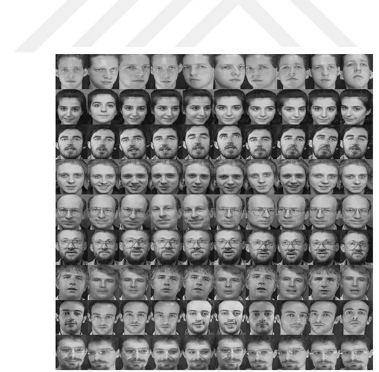
ORL face database consists of 400 images taken in laboratory environment (Samaria and Harter, 1994). The database was established within the framework of a facial recognition project in collaboration with the Engineering Department of Cambridge University. Ten different images of each of the 40 individual subjects were taken. The images were taken in different lighting conditions, different facial expressions (open and closed eyes, smiling and not smiling) and different facial details (with and without glasses) at different times. The photo shootings were made on the same floor in the same place with the people in the upright position and in the front position. Images are taken in PGM (Portable Gray Map) format. Image sizes are 92x112 pixels. Sample images in the database are shown in Figure 3.1.
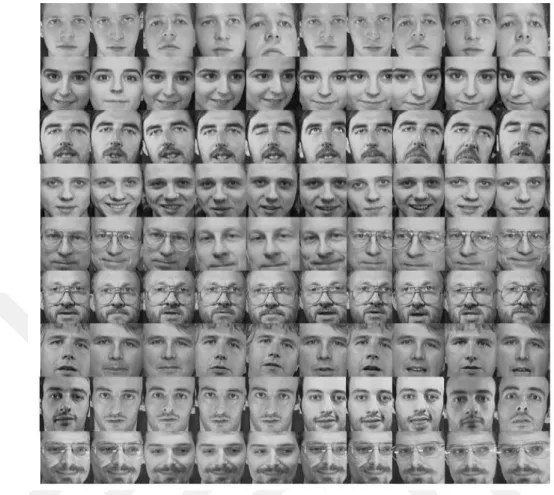
When looking at the sample images the hair and background information create noise. Only the facial portion was obtained from the images for the use of facial expressions. The images obtained as a result of the cropping process are given in Figure 3.2.
11
Figure 3. 2. Cropped images of sample images in ORL database
3.2. Methods
In this section, at first classical LBP and then the two proposed LBP based methods are explained in detail. The first proposed method is based on relations between neighborhood, called nLBP, and other is based on angles, which is called αLBP.
3.2.1.Conventional Local Binary Pattern Operator
The Local Binary Pattern (LBP) is a statistical approach that allows us to obtain effective properties from images (Yang and Chen, 2013). LBP feature extraction is based on local neighborhood values. It is widely used in computer vision applications. Its effectiveness has been proven by various applications. It consists of two stages. In the first stage, local binary patterns from the images produce microstructures. The second stage is the histogram of these patterns (Ojala et al., 2002; Liu et al., 2016).
12
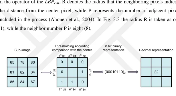
LBP identifier creates a binary value for each pixel by comparing the pixels around the center pixel in the vicinity of 3x3 (Yang et al., 2016). An example of labeling a pixel with the LBP identifier is given in Figure 3.3. LBP values are obtained by duplicating the difference between the neighbors of each pixel in the image with the step function (Equation 3.1) (Gu and Liu, 2013; El Khadiri et al., 2018).
∑ {
(3.1)
In the operator of the LBPP,R, R denotes the radius that the neighboring pixels indicate
the distance from the center pixel, while P represents the number of adjacent pixels included in the process (Ahonen et al., 2004). In Fig. 3.3 the radius R is taken as one (1), while the neighbor number P is eight (8).
Thresholding according comparison with the center
65 78 80 81 82 84 85 84 67 8 th b it
1th bit 2nd bit 3th bit
4
th
b
it
7th bit 6th bit 5th bit
8 bit binary representation 0 0 0 0 1 1 1 0 (00010110)2 22 Decimal representation Sub-image
Figure 3. 3.Calculation of LBP code (Kaya et al., 2015)
In the studies, most of the patterns in the images are composed of uniform type. The uniform patterns are those with 0 or 1 or 1 to 2 passages in the binary LBP code. For example, the patterns 00000000 and 11111111 are 0 in the 0 pass, 01100000 and 11000011 are 2 patterns in pattern. Uniform patterns may represent simple textures such as spot, edge, and corner. In total there are (P-1) P + 2 uniform patterns (Kaya et al., 2015).
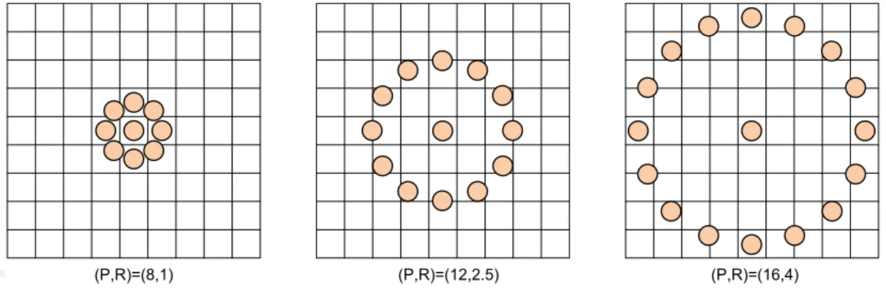
The first parameter of LBP is P, which indicates the neighbor number. In the creation of the LBP image, the large values of P both increase the attribute histogram and increase the cost of processing. Minor values of P may cause significant loss of information (Smolka and Nurzynska, 2015). The second parameter of LBP is the radius (R) parameter. R indicates the distance of between the neighbor and center pixels. With
13
the use of different R values, one can perform the texture analysis at different sizes. Using different P and R values, it is possible to perform multi-scale texture analysis (Lumini et al., 2017). Figure 3.4 shows examples of different LBP operators with different P and R values.
(P,R)=(8,1) (P,R)=(12,2.5) (P,R)=(16,4)
Figure 3. 4. Circularly symmetric neighbor sets for different LBP operators (Kaya et al., 2015).
3.2.2. Local binary patterns based on relations between neighbors: neighborliness LBP
nLBPd is generated based on the relationship between the neighbors around each pixel. 8 adjacent P = {P0, P1, P3, P3, P4, P5, P6, P7} around each pixel are taken as a decimal equivalent of the binary index obtained from the comparisons between neighbors (Kaya et al., 2015). If a pixel is greater than the next pixel in comparisons, “1” is taken as “0” in other cases. An example of nLBPd is given as follows. nLBPd has a parameter in the form of distance (d). This parameter specifies the distance between sequential neighbors to be compared. Different patterns are obtained for different values of d. Figure 3.5 shows examples of how the LBP forms a double pattern from different distances.
14
Figure 3.5 (A) shows a part of an image. Figures 3.5 (B), 3.5 (C) and 3.5 (D) show the adjacent pixels to be compared in cases where the distance (d) is 1, 2 and 3 in the nLBP method, respectively.
The nLBP method depends on the pixels P selected around each pixel. Examples are given below for d = 1, d = 2 and d = 3, where Pc is the center pixel and P = {P0, P1, P2, P3, P4, P5, P6, P7} are the neighbors around the center pixel.
T=(Pc, P0,P1,P2,P3, P4, P5, P6, P7)
Pc=S(P0>P1),S(P1>P2),S(P2>P3),S(P3>P4),S(P4>P5),S(P5>P6),S(P6>P7),S(P7>P0) (3.2)
{
(3.3)
If Pi> Pj is “1”, in other cases “0” is taken.
The calculation of nLBP for d = 1 is shown below (Figure 5 (B)). Pc=50>82|82>30|30>64|64>57|57>98|98>85|85>61|61>50 Pc=0,1,0,1,0,1,1,1
Pc=(01010111)2=(87)10
Calculation of BPd for d = 2 (Figure 3 (C)).
Pc=S(P0>P2),S(P1>P3),S(P2>P4),S(P3>P5),S(P4>P6),S(P5>P7),S(P6>P0),S(P7>P1) (3.4)
Pc=50>30|82>64|30>57|64>98|57>85|98>61|85>50|61>82 Pc=1,1,0,0,0,1,1,0
Pc=(11000110)2=(198)10
Calculating nLBPd for d = 3 (Figure 3 (D)).
Pc=S(P0>P3),S(P1>P4),S(P2>P5),S(P3>P6),S(P4>P7),S(P5>P0),S(P6>P1),S(P7>P2) (3.5)
Pc=50>64|82>57|30>98|64>85|64>61|98>50|85>82|61>30 Pc=0,1,0,0,1,1,1,1
15
As seen above, different patterns were obtained for different d parameter values.
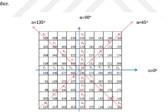
3.2.3. Local Binary Patterns based on angles : αLBP
The basic idea behind the LBP is that it assumes that an image is made of micro-patterns. The histogram of these microstructures includes information on the distribution of local characteristics in an image. Angle values are one of the degrees (α = 0, 45, 90 and 135). The neighbors (P = {P0, P1, P3, P3, P4, P5, P6, P7) are evaluated on the plane drawn over the center pixel (Pc) according to an angle value.
The center pixel is compared with the remaining neighbors on the drawn plane and A is labeled as 1 if Pc>Pi and in other cases 0. Then the decimal value of the binary string obtained is taken as the value of the center pixel. αLBP is calculated as:
i P i c i P P u aLBP ( )2 0
(3.6)As shown in Figure 3.6, the LBP operator is calculated for two horizontal and two vertical angles. LBP operators calculated according to different angles differ from each other.
Figure 3. 6. Overview of αLBP (Kaya et al., 2015)
It is thought that the method of searching patterns with different angles will provide success in different texture problems. LBP operators obtained from different angles according to Figure 3.6 are given below.
16 Calculation
aLBP
for α = 0;Pc=S(P0>Pc),S(P1>Pc),S(P2>Pc),S(P3>Pc),S(P4>Pc),S(P5>Pc),S(P6>Pc),S(P7>Pc) (3.7) Pc=S(217>210),S(255> 210),S(255> 210),S(241> 210),S(181> 210),S(177> 210),S(146> 210),S(119> 210)
Pc=0,0,0,0,1,1,1,1 Pc=(00001111)2=(15)10
Calculation
aLBP
for α = 45;Pc=S(P0>Pc),S(P1>Pc),S(P2>Pc),S(P3>Pc),S(P4>Pc),S(P5>Pc),S(P6>Pc),S(P7>Pc) (3.8) Pc=S(117>210),S(138> 210),S(146> 210),S(157> 210),S(212> 210),S(171> 210),S(172> 210),S(169> 210)
Pc=1,1,1,1,0,1,1,1 Pc=(11110111)2=(247)10 Calculation
aLBP
for α=90;Pc=S(P0>Pc),S(P1>Pc),S(P2>Pc),S(P3>Pc),S(P4>Pc),S(P5>Pc),S(P6>Pc),S(P7>Pc) (3.9) Pc=S(167>210),S(146> 210),S(145> 210),S(153> 210),S(162> 210),S(143> 210),S(134> 210),S(150> 210)
Pc=1,1,1,1,1,1,1,1 Pc=(11111111)2=(255)10
Calculation
aLBP
for α=135;Pc=S(P0>Pc),S(P1>Pc),S(P2>Pc),S(P3>Pc),S(P4>Pc),S(P5>Pc),S(P6>Pc),S(P7>Pc) (3.10) Pc=S(162>210),S(129> 210),S(188> 210),S(165> 210),S(196> 210),S(155> 210),S(150> 210),S(129> 210)
Pc=1,1,1,1,1,1,1,1 Pc=(11111111)2=(255)10
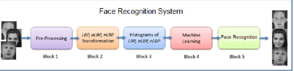
17 3.3. Proposed Face Recognition System
Face recognition systems consist of several stages. Usually consists of feature extraction and classification operations. The recommended system for face recognition is given in Figure 3.7. The proposed system consists of 5 stages. The steps are summarized below.
Figure 3. 7. Face Recognition System
Block 1: At this stage, only the facial parts are cropped from images. The success of facial recognition systems depends on the clean, complete reception of the facial expression. Therefore, the clean face is cropped after face detection before images. Block 2: LBP, nLBP and αLBP methods were applied to facial images. At this stage, LBP face images are created.
Block 3: Histograms of LBP, nLBP and αLBP facial images are generated. Each value in the histogram refers to a pattern. These patterns are used as features for machine learning methods.
Block 4: kNN and Artificial Neural Networks (ANN) classification methods were used at this stage. Classification procedures were performed according to 10-fold cross validation test. The accuracy of the system is the classification average of these 10 trials.
Block 5: The accuracy calculations are made at this stage.
3.3.1. Classification Methods
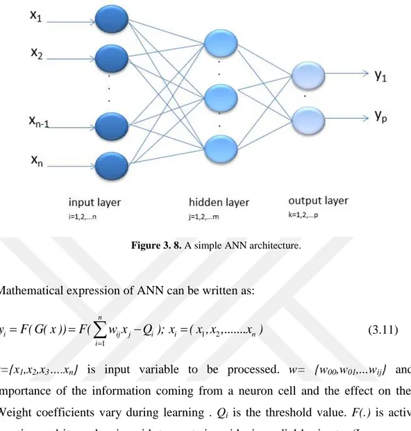
3.3.1.1. Artificial Neural Networks (ANN)
ANN is a popular method in machine learning. An ANN model consists of an input layer, one or more hidden layers and an output layer (Jain A.K. et al.; Karungaru et al, 2002). An example ANN model is shown as in Figure 3.8. The circles show the artificial neurons and the lines show the weight coefficients. Lines represent the data transfer path between the neurons from different layers (Singh et al, 2002).
18
Figure 3. 8. A simple ANN architecture.
Mathematical expression of ANN can be written as:
1 2 1 n i ij j i i n i y F( G( x )) F( w x Q ); x ( x ,x ,...x )
(3.11)x={x1,x2,x3….xn} is input variable to be processed. w= {w00,w01,...wij} and the
importance of the information coming from a neuron cell and the effect on the cell. Weight coefficients vary during learning . Qi is the threshold value. F(.) is activation
function and it can be sigmoid, tangent sigmoid, sin, radial basis etc. (Lawrence et al., 1997). Different layers of an ANN can have the same or different activation function. 3.3.1.2. kNN Method
kNN method, one of the data mining classification methods, was first introduced by Fix and Hodges (1989) as a nonparametric method for use in pattern recognition and was later developed by Cover and Hart (1967). It is one of the supervised machine learning algorithms that make classification based on observations. It is one of the nonparametric methods and it has a simple and easy interpretation. It is used in many areas such as pattern recognition, artificial intelligence, data mining, statistics, cognitive psychology, medicine, bioinformatics (Cunningham and Delany, 2007).
The K-closest neighbor algorithm makes classification using distance or proximity calculation. Briefly, the classification algorithm is based on the idea that
19
"objects close to each other in the sample space probably belong to the same category". The purpose of the algorithm is to assign individuals or objects to the predefined classes or groups in the most appropriate way by using the properties of these objects. The method provides a classification of a new observation. The observation that is intended to be classified is based on the classification of the same dataset as the one belonging to the maximum number of units from the nearest unit with the help of the learning data set. The data set formed by the data to be used in the formation of a model is called the learning data set (Teknomo, 2012).
3.4. kNN algorithm steps
kNN algorithm is used to classify observations based on similarities to other cases. The model was developed as a way of recognizing data models in learning, without exact matching to stored patterns or cases. Similar observations are close to neighbors. Thus, the distance between the two observations is a criterion that identifies each other. When a new observation is presented, the distance from each observation in the model is calculated. The new observation is assigned to the most similar category.
In applying this method;
• The distance between the new observation and all observations in the data set is calculated,
• These distances are sorted from large to small, • k Observations with k smallest distance values,
The weighted voting method can also be used instead of finding the class value with the most recurring category in the observation. The opposite is used as weight (Equation 3.12). With the help of the weights calculated for each class, the category with the highest weight is available as the class value. By observing observations in the learning data set (xi) and observations in the test sample (xq) it is possible to increase the distance of the most closely observed observations by using Equation (3.12) to become kNN (Zhou et al., 2009).
Before starting the classification process, it is necessary to convert all the data to numerical values and determine how many neighbors (k) should be taken. When determining the class of observations in the test sample, the distances to the
20
observations in the learning data set are calculated and the closest k observations are selected. For distance calculation, Euclidean, Manhattan, Minkowski, Chebyshev, Dilca methods can be used.
3.4.1. Pre-processing of data
kNN algorithm, optionally data; Learning eye (training)” test hold (holdout) data set. The learning data set is used in the formation of the model. The test data is used to evaluate the model independently. Missing observations in continuous variables can be ignored. Categorical variables have the option of evaluating missing observations. The number of categories can be reduced by combining similar categories or by subtracting the lesser observed categories before the model is applied. In addition, contrary observations can also be omitted from the model. The answer variable in the kNN algorithm can be categorical or continuous (Zhou et al., 2009).
When kNN is used to classify observations in a continuous structure, an approximate (mean or median) value of the nearest neighbors is used to estimate the classification of a new observation. kNN algorithm optionally estimates scale continuity before re-scaling (normalizing) variables before training the model. The normalization of continuous observations is given in Equation (3.13) (Zhou et al., 2009).
( )
( ) In Equality (3.13); xpn, n normalized value of observation, x0p, n original value
of observation, min(x0p), minimum value of observation and max for all learning
situations (x0p), the maximum value of the observation for all learning situations.
In forward-looking algorithm, forward selection method is used in variable selection of algorithm. Variables are selected in order, and the feature selected at each step must be the variable that ensures that the error rate or sum of error squares is minimum (Cunningham and Delany, 2007).
3.4.2. K number and its effect on classification
kNN uses the nearest neighboring examples to classify or estimate observations in the n-dimensional property space. The number of closest neighbors to be considered in order to classify the new observation is indicated by a positive integer such as k. If k
21
= 1, the new observation is going to be included in the class of the nearest neighbor. This method is also used for estimation. When all the data in the data set are taken into account, the most repetitive category is assigned. In short, k is the number that indicates how many nearest neighbors should be considered for the classification of a new observation.
3.4.3. Cross validity test
One of the common methods used to test the accuracy of a model is the cross validity test. This test can also be preferred if a limited number of data is available. In this method, the data set is randomly divided into two or more groups. In the first stage, the model is learned on one of the groups and the test is performed on the other. In the second stage, the model and test groups are displaced and the mean error rates are used. In databases with a sample width of several thousand or less, n-fold cross validation test, where data are divided into n groups, may be preferred. For the cross validity test, it is observed that the most preferred n value in the literature is 10. If the data are divided into 10 groups, the first group is used for the first group test and the other groups for the learning. This process is carried out each time a group is tested, and other groups are used for learning purposes. The average of the 10 error rates obtained will be the estimated error rate of the established model (Berson et al., 1999). When the number of the nearest neighbor is determined automatically; error rate, kmin to kmax between the values. Assuming that the learning data set (1, 2, ..., n) is a variable with integer values, the cross validity test (CVk) equality will be:
∑
any k∈(kmin,kmax) for , average error rate or error squares sum (en/n) calculated. Optimal
k equation (3.15) is selected as follows:
̂ { } If more than one k value is associated with the lowest average error rate, the smallest of them is selected.
22 3.4.5. Performance Measures
The metrics for performance measurement are error rate, precision, sensitivity and F-criterion. The criteria used to measure model success are obtained from the confusion matrix below.
Table 3. 1. Performance criteria
Actual
Predicted Class 1 Class 0
Class 1 TP (True Positive) FP (False Positive)
Class 0 FN (False Negative) TN (True Negative)
True Positive: Specifies the number of samples when the prediction and the actual value are both Class 1.
True Negative: Specifies the number of samples when the prediction and the actual value are both Class 0.
False Positives: Specifies the number of samples when the prediction is Class 1 but the actual value is Class 0.
False Negative: Specifies the number of samples when the prediction is Class 0 but the actual value is Class 1.
3.6. Accuracy
Accuracy is the ratio of the number of accurately classified samples (TP + TN) to the total number of samples (TP + TN + FP + FN).
Accuracy = TP+TN/TP+FP+FN+TN (3.16)
3.7. Error rate
The error rate is the ratio of the number of incorrectly classified samples (FP + FN) to the total number of samples (TP + TN + FP + FN).
Error rate = FP+FN / TP+FP+FN+TN (3.17)
OR
23 3.8. Precision
Precision is given as:
Precision = TP / TP+FP (3.19)
3.8.1. Recall Recall is given as:
Recall =TP / (TP + FN) (3.20)
3.8.2. F-measure
Combining both precision and recall criteria together enables more accurate interpretation. F-measure is given as:
24 4. RESULTS
In this thesis, two novel approaches, nLBP and αLBP, based on LBP were used for face recognition problem. The results obtained by nLBP, αLBP and classic LBP are given. Results from these approaches were compared.
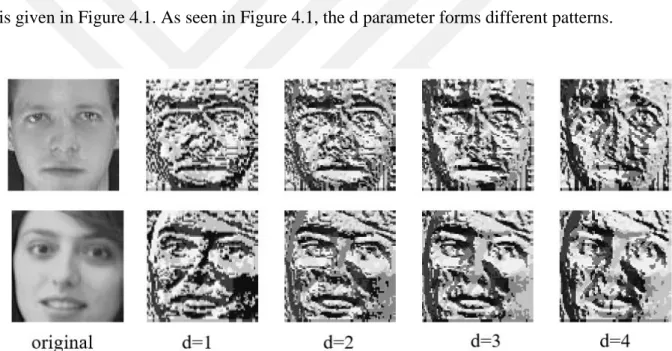
4.1. Results for nLBP (neighborliness Local Binary Pattern)
The success of facial recognition systems depends on the effectiveness of features extracted from face images. Extracted geometric or textural features affect the success of the classification method. In this section the effectiveness of nLBP method in face recognition is given. The nLBP method depends on the d (distance) parameter. Different features are obtained according to the value of this parameter. The effect of the d parameter on two images (one male and one female) from the ORL face database is given in Figure 4.1. As seen in Figure 4.1, the d parameter forms different patterns.
Figure 4. 1. Formed faces according to different d values with nLBP method.
Figure 4.1 shows that different facial images are formed according to different values of parameter d. The histograms of the nLBP facial images were also examined and given in figure 4.2. It can be seen from the histograms that as the value of the d parameter increases, the important patterns begin to disappear. The pattern distribution is shifted to the left and right. For both images, it is clear that the pattern distributions change when the value of d increases.
25
Figure 4. 2. nLBP method histograms of faces formed by different values of parameter d
Classification was performed with kNN and ANN by using the features obtained with nLBP. The classification process was performed with the Weka open source data mining tool (Frank et al., 2016). The results obtained according to 10-fold cross validation test are given in Table 4.1. In addition, the success rates obtained with kNN and ANN according to different distance (d) values are given in Figure 4.3.
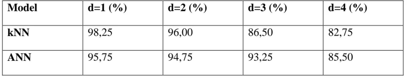
Table 4. 1. Results obtained with kNN and ANN for nLBP
Model d=1 (%) d=2 (%) d=3 (%) d=4 (%)
kNN 98,25 96,00 86,50 82,75
26
Figure 4. 3. Accuracy results according to different distance (d) values
As can be seen from Table 4.1, high accuracy results were obtained by both kNN and ANN. The highest success rate was obtained with kNN as 98.25% in the case of d (d = 1). The lowest success rate with kNN was observed as 82.75% with d = 4. In general, as the value of the d parameter increases, the success rate decreases. This supports the loss of patterns as the d value increases. However, we need to look at the different values of the d parameter.
Performance measures observed with kNN and ANN are given in Table 4.2 and Table 4.3. The most popular measures for measuring model performance are given.
Table 4. 2. Performance measures obtained with kNN for nLBP features
D Precision Recall F-Measure Error Rate
d=1 0,984 0,983 0,982 0,0175 d=2 0,969 0,960 0,960 0,0400 d=3 0,880 0,865 0,864 0,1350 d=4 0,840 0,830 0,830 0,1725 81 84,25 79,5 82,75 81,5 87,45 88,5 83,75 1 2 3 4
Accuracy Rates
Knn ANN27
Table 4. 3. Performance measures obtained with ANN for nLBP features
d Precision Recall F-Measure Error Rate
d=1 0,963 0,958 0,957 0,0425
d=2 0,951 0,948 0,947 0,0525
d=3 0,939 0,933 0,930 0,0675
d=4 0,864 0,855 0,854 0,1450
As seen in Table 4.2 and Table 4.3 the highest success rates were obtained when d = 1.
4.2. Results for αLBP
αLBP is the other method used in this thesis. The success of the methods depends on the discrimination strength of the features extracted from face images. This method has only one parameter. The α parameter is the angle parameter. αLBP operator calculates the value of each pixel according to an angle value. Angle values can be α=0, 45, 90 or 135. The basic idea behind αLBP is that it assumes that an image consists of micro-patterns. The histogram of these micro-patterns includes information on the distribution of local characteristics in an image. αLBP images of two face images with α = 0, 45, 90 and 135 are shown in Figure 4.4.
28
Figure 4.4 shows that different facial images are formed according to the different values of the α parameter. To see this in more detail, histograms of newly formed αLBP facial images need to be examined. In Figure 4.5, histograms of face images are given. As seen from the histograms, it is seen that the patterns differ as the value of the α parameter changes.
Figure 4. 5. αLBP histograms of faces formed by different values of α parameter
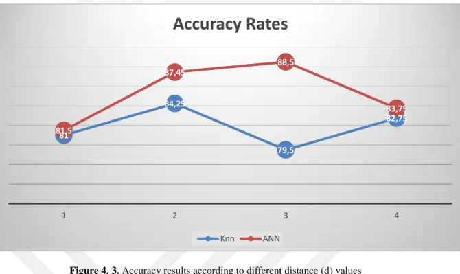
For the patterns obtained with αLBP, classification with kNN and ANN was performed. The classification process was carried out according to 10-fold cross validation test. The success rates are given in Table 4.4. In addition, the success rates obtained according to the angle (α) values are given in Figure 4.6.
29
Table 4. 4. Accuracy rates with kNN and ANN classification methods for αLBP features
Model α=0 α=45 α=90 α=135
kNN 81,00 84,25 79,50 82,75
ANN 81,50 87,45 88,5 83,75
Figure 4. 6. Success rates according to different angle values
As can be seen from Table 4.4, acceptable results were observed at the intermediate level with both kNN and ANN. The highest success rate was achieved as 88,5% with ANN in of cases α =90.The lowest success rate with kNN was 79,50% in case of α =90. The α value should be decided by trials. The success rate of the α parameter does not depend on the small or large value. At the end of the experiments, the effective α value can be observed. Performance measures observed with kNN and ANN are given in Table 4.5. and Table 4.6. For measuring the performance of models the most popular criteria are used.
81 84,25 79,5 82,75 81,5 87,45 88,5 83,75 0 45 90 135
Accuracy Rates
Knn ANN30
Table 4. 5. Performance measures obtained with kNN for αLBP
α Precision Recall F-Measure Error Rate
α=0 84,5 81,0 80,3 19,0
α=45 87,2 84,3 83,7 15,75
α=90 75,66 79,5 80,03 20,50
α=135 86,54 82,80 82,21 17,25
Table 4. 6. Performance measures obtained with ANN for αLBP
α Precision Recall F-Measure Error Rate
α=0 85,00 81,25 80,4 18,5
α=45 88,90 86,30 89,40 12,55
α=90 91,25 87,50 90,02 11,50
α=135 86,80 83,00 83,20 16,25
4.3. Results for Classic LBP
The proposed methods are compared with the classical LBP method. While a single set of features is obtained from the facial images with the classic LBP, different feature groups are obtained according to the d and α parameters in nLBP and αLBP methods. The face images obtained by applying the LBP method to two different images are given in Figure 4.7.
31 Histograms of LBP faces are given in Figure 4.8.
Figure 4. 8. Histograms of LBP faces
Using the features obtained by the LBP method, the classification was performed with kNN and ANN. The success rates and performance measures are given in Table 4.7.
Table 4. 7. Performance measures obtained with kNN and ANN for LBP
Model Accuracy Precision Recall F-Measure Error Rate
kNN 74,25 0,773 0,743 0,742 15,75
ANN 83,5 0,832 0,835 0,828 16,5
Looking at the results for LBP, a success rate of 83,5% was observed with ANN. A lower success rate was obtained with kNN. In terms of general success rates, ANN was observed to be more successful than kNN.
32 4.5. Comparison of Models
The proposed nLBP and αLBP methods were compared with the classical LBP and its uniform features groups. All performance measures are given in Table 4.8.
Table 4.8. Comparison of methods
Features+Classifier Accuracy Precision Recall F-Measure Error Rate
nLBPd=1+(kNN) 98,25 0,984 0,983 0,982 1,75 αLBPα=90 + (ANN) 88,50 0,9125 0,8750 0,9002 11,50 LBP +(ANN) 83,50 0,832 0,835 0,828 16,5 +ANN 93,00 0,937 0,930 0,929 7,0 +ANN 89,75 0,904 0,898 0,888 10,25 LBPU2+ANN 79,25 0,810 0,793 0,787 80,75
As seen in Table 4.8, the highest success rate was 98,25% with nLBPd=1 + (kNN). The lowest success rate was observed with LBPU2 + ANN. In this thesis, the proposed methods of nLBP and αLBP were found to be more successful than the classical LBP method. The nLBP method was more successful than the αLBP method.
4.6. Comparison of Different Machine Learning Methods
In this thesis, kNN and ANN were used as the classification methods. nLBP, αLBP and LBP features were used for different machine learning methods except kNN and ANN. The classification was performed according to Weka open source program with 10-fold cross validation method. The success rates obtained by Support Vector Machine (SVM), Naïve Bayes (NB), Functional Tree (FT) and Bayes Net (BN) methods are given in Table 4.9 (Gama, 2004; Friedman et al. 1997). In the table, the kNN and ANN methods used in this study were found to be more successful than other methods.
33
Table 4.9. Performance measures obtained by different machine learning methods
Features kNN ANN SVM NB FT BN nLBPd=1 98,25 95,75 88,00 89,25 93,75 87,25 LBPα=90 79,50 88,50 86,00 77,00 74,50 76,75 LBP 74,25 83,50 80,75 76,25 72,50 74,75 88,00 93,00 87,00 86,75 77,50 78,50 75,75 89,75 82,25 72,50 81,25 71,25 LBPU2 79,25 79,25 75,25 76,75 72,50 76,00
4.7. Comparison with the Studies in Literature
A part of the studies in literature using the ORL face database is given in Table 4.10. Different machine learning or feature extraction methods are used. In the table, it is seen that the proposed nLBP and αLBP feature extraction methods produced more successful results.
Table 4. 10. Studies using the ORL face database
Author(s)/Year Model Accuracy(%)
Wright et al., 2009
SRC, sparse representation based classification
80,00 Zhang et al., 2012 CRC, Collaborative representation based classification 90,00 Naseem et al.,
2010
LRC, Linear Regression Classification 83,75
Deng et al., 2012 Extended SRC 80,23
Xu et al., 2011 TPTSR 93,75
Wang et al., 2017 Synthesis linear classifier based analysis 83,33
Lu et al., 2012 Incremental complete LDA 86,75
He et al., 2005 Laplacian faces 91,33
Song et al., 2019 Weighted LBP 93,75
34 5. CONCLUSION
As a classic pattern recognition problem, face recognition primarily consists of two critical sub-problems. The first is the feature extraction from facial images, and the second is the classifier design. The classification success depends on the effectiveness of the acquired features. The attributes obtained from the facial images can be grouped into either holistic or local features. The holistic features uses the entire face region and represent the entire face image. The holistic features do not capture local variations in the face view (Liu et al., 2016). In contrast, the local features capture the local characteristics from the image. Face images are classified by combining and comparing the sub-region of a face and then with the relevant local statistics. LBP is one of the most prominent methods in the local attributes approach. LBP is one of the simplest statistical approaches used for texture analysis (Ojala et al., 2002). LBP compares each pixel in the image with the adjacent pixels around the pixel (Pan et al., 2017).
In LBP approach, it is assumed that the central pixel and its neighbors are independent, and the relationships between these pixels are encoded as binary patterns. Despite the success of LBP in computer vision applications especially in face recognition, the traditional LBP has some disadvantages. (1) long unevenly distributed histograms are produced. (2) pattern depends on rotation, (3) Noise-sensitive (4) large-scale textures are difficult to detect. This situation makes it difficult to obtain effective properties (Tian et al. 2011; Pietikäinen et al., 2011). To overcome these issues, different LBP methods are suggested.
Two new approaches: nLBP and αLBP together with classical LBP were used in this study. nLBP is formed according to the relationship between the neighbors around each pixel. The nLBP has a distance parameter (d). This parameter specifies the distance between consecutive neighbors to be compared. Different patterns for different d parameter values are obtained. The αLBP operator calculates the value of each pixel according to an angle value. Angle values can be α = 0, 45, 90 or 135 degrees.
In this thesis, the features extracted with LBP, nLBP and αLBP from face images in ORL database and were classified by using kNN and ANN. Using LBP attributes, success rates of 74.25% and 83.5% with ANN were obtained with kNN (Table 4.7).
In the nLBP method, different results are obtained by changing d parameter. The success rates obtained by using the d (distance) parameter according to the different
35
values of d = {1,2,3,4} are as follows: kNN = {98.25%, 96.00%, 86.50%, 82.75%} and ANN = {95.75%, 94.75%, 93.25%, 85.50%} (Table 4.1). As the value of the distance (d) parameter increases, the success rate decreases. The αLBP method has α angle parameter. The success rates obtained by using the values obtained by the values of α = {0,45,90,135} were observed as kNN = {81.00%, 84.25%, 79.50%, 82.75%} and ANN = {81.50%, 87.45%, 88.50%, 83.75%}, respectively (Table 4.4).
In conclusion, it is shown that the new nLBP method gives higher accuracy results when compared to classical LBP and αLBP methods for face recognition problem. The face recognition system was designed using the face images in the ORL face database. In the future, we plan to test these new LBP methods using bigger face datasets.