Gibbs model based 3D motion and structure estimation for object-based video coding applications

We also proposed a vector prediction based fast motion estimation algorithm for reducing the energy consumption of H.264 MVC motion estimation hardware by utilizing the

To select the required machine precision for any MP-MLFMA tree structure, as well as to control the translation errors due to the truncation of the diagonal form of the

Figure 5.10: Original average target ERP signal a, composite time–frequency representation obtained by TFCA b and estimated individual time–domain components c and d for the

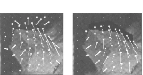
AMD, cis its name implies, is an algorithm which finds the average motion between two video frames and thus finds the amount of change within two frames. In

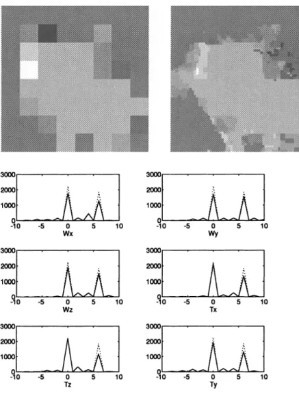
To see how the algorithm behaves in case of large motion, we increase u>x and plot the percentage estimation error in versus ujx with considering the

Patients (Expanded Disability Status Scale [EDSS] score ≤4.0; disease duration ≤10 years; discontinued prior DMT of ≥6 months’ duration due to suboptimal disease control)

While we find no obvious candidates in human low and mid-level visual cortex for an explicit representation of specular reflectance from motion, we do find several areas with

We studied human-in-the-loop physical systems with uncertainties due to failures and/or modeling inac- curacies, a set-theoretic model reference adaptive control law at the inner

REFERENCES

[1] J.K. Aggarwal and N. Nandhakumar, "On the computation of motion from image sequences-a review," IEEE Proc., vol. 76, pp. 917-935, Aug. 1988.
[2]
A. Verri and T. Poggio, "Motion field and optical flow: Qualitative properties," IEEE Trans. Pattern Anal. Machine Intell., vol. 11, pp.
490-498, May 1989.
[3] R.Y. Tsai and T.S. Huang, "Uniqueness and estimation of three-dimensional motion parameters of rigid objects with curved surfaces," IEEE Trans. Pattern Anal. Machine Intell., vol. 6, pp. 13-27, Jan. 1984.
(34)
[4] K. Aizawa and T.S. Huang, "Model-based image coding: Advanced video coding techniques for very low bit-rate applications," IEEE Proc., vol. 83, pp. 259-271, Feb. 1995.
[5] G. Bozdagl, Three Dimensional Facial Motion and Structure Estimation
in Video Coding. PhD thesis, Bilkent University, Jan. 1994.
[6] H. Li, P. Roivainen and R. Forchheimer, "3-d motion estimation in model-based facial image coding," IEEE Trans. Pattern Anal. Machine
Intell., vol. 15, pp. 545-555, June 1993.
[7] J.O. Limb and J.A. Murphy, "Measuring the speed of moving objects from television signals," IEEE Trans. Commn., vol. , pp. 474-478, April 1975.
[8] C. Cafforio and F. Rocca, "Methods of measuring small displacement of television images," IEEE Trans. Inform. Theo., vol. 22, pp. 573-579, Sep. 1976.
[9] B.K.P. Horn and B.G. Shunck, "Determining optical flow," Artificial
Intell., vol. 17, pp. 185-203, 1981.
[10] A.M. Tekalp, Digital Video Processing. Prentice Hall, 1995. [11] A.N. Netravali and J.D. Robbins, "Motion-compensated television
coding, part-I," AT fj T Techn. Jour., vol. 58, pp. 629-668, March 1979.
[12] J.R. Jain and A.K. Jain, "Displacement measurement and its application in interframe image coding," IEEE Trans. Commun., vol. 29, pp.
1799-1808, Dec. 1981.
[13] M. Bierling, "Displacement estimation by hierarchical blockmatching," in Proc. of SPIE Visual Commun. and 1m. Proc. 88, pp. 942-951, 1988. [14] V. Seferidis and M. Ghanbari, "General approach to block-matching
motion estimation," Optical Engineering, vol. 32, pp. 1664-1474, July 1993.
[15] J. Hutchison, C. Koch, J. Luo and C. Mead, "Computing motion using analog and binary resistive networks," IEEE Trans. Computer, vol. , pp. 52-63, March 1988.
[16] S. Geman and D. Geman, "Stochastic relaxation, Gibbs distributions, and the Bayesian restoration of images," IEEE Trans. Pattern Anal.
(35)
[17] J. Konrad and E. Dubois, "Bayesian estimation of motion vector fields,"
IEEE funs. Pattern Anal. Machine Intell., vol. 14, pp. 910-927, Sep.
1992.
[18] F. Heitz and P. Bouthemy, "Multimodal motion estimation and segmentation using Markov random fields," in Proc. Int. Conf. on Pat.
Recog. 90, pp. 378-383, 1990.
[19] F. Heitz and P. Bouthmey, "Multimodal estimation of discontinuous optical flow using Markov random fields," IEEE funs. Pattern Anal.
Machine Intell., vol. 15, pp. 1217-1232, Dec. 1993.
[20] R. Buschmann, "Joint multigrid estimation of 2d motion and object boundaries using boundary patterns," in SPIE Visual Commun. and
Image Proc. 93, pp. 106-118, 1993.
[21] S. Iu, "Robust estimation of motion vector fields with discontinuity and occlusion using local outliers rejection," in SPIE Visual Commun. and
Image Proc. 93, pp. 588-599, 1993.
[22] E. Dubois and J. Konrad, "Motion estimation and motion-compensated filtering of video signals," in Proc. of IEEE ICASSP 93, pp. 95-98, 1993. [23] R. Depommier and E. Dubois, "Motion estimation with detection of
occlusion areas," in Proc. of IEEE ICASSP 92, pp. 269-272, 1992. [24] C.L. Chan, J.C. Brailean, A.K. Katsaggelos and A.V. Sahakin,
"Maximum a posteriori displacement field estimation in quantum-limited image sequences," in SPIE Visual Commun. and Image Proc. 93, pp. 396-407, 1993.
[25] J.C. Brailean and A.K. Kataaggelos, "Recursive map displacement estimation and restoration of noisy-blurred image sequences," in SPIE
Visual Commun. and Image Proc. 93, pp. 384-395, 1993.
[26] S. Kirkpatrick, C.D. Gelatt and M.P. Vecchi, "Optimization by simulated annealing," Science, vol. 220, pp. 661-680, 1983.
[27] J. Besag, "On the statistical analysis of dirty pictures," J.R. Statist.
Soc., vol. 48, pp. 259-302, 1986.
[28] F. Heitz, P. Perez and P. Bouthemy, "Multiscale minimization of global energy functions in some visual recovery problems," CVGIP: Image
(36)
[29] W.N. Martin and J.K. Aggarwal, Motion Understanding, Robot and
Human Vision, pp. 329-352. Kluwer Academic Publishers, Boston, 1988. [30] J.F. Vega-Riveros and K. Jabbour, "Review of motion analysis
techniques," lEE Proc., vol. 136, pp. 397-404, Dec. 1989.
[31] J.N. Driessen, Motion Estimation for Digital Video. PhD thesis, Delft University of Technology, Sep. 1992.
[32] M.l. Sezan and R. L. Lagendijk, ed. Motion Analysis and Image
Sequence Processing. Kluwer Academic Publishers, 1993.
[33] R.Y. Tsai and T.S. Huang, "Estimating three-dimensional motion parameters of a rigid planar patch," IEEE Trans. Sig. Proc., vol. 29, pp. 1147-1152, Dec. 1981.
[34] X. Hu and N. Ahuja, "Sufficient conditions for double and unique solution of motion and structure," CVGIP: Image Understanding, vol. 58, pp. 161-176, Sep. 1993.
[35] J.W. Roach and J.K. Aggarwal, "Determining the movement of objects from a sequence of images," IEEE Trans. Pattern Anal. Machine Intell., vol. 2, pp. 554-562, Nov. 1980.
[36] S. Ullman, "Maximizing rigidity: The incremental recovery of 3d structure from rigid and nonrigid motion," Perception, vol. 13, pp. 255-274, 1984.
[37] A. Pentland and B. Horowitz, "Recovery of nonrigid motion and structure," IEEE Trans. Pattern Anal. Machine Intell., vol. 13, pp. 730-742, July 1991.
[38] D. Terzopoulos and D. Metaxas, "Dynamic 3d models with local and global deformations: Deformable superquadrics," IEEE Trans. Pattern
Anal. Machine Intell., vol. 13, pp. 703-714, July 1991.
[39] C. W. Chen, T. S. Huang and M. Arrott, "Modelling, analysis, and visualization of left ventricle shape and motion by hierarchical
decomposition," IEEE Trans. Pattern Anal. Machine Intell., vol. 16, pp. 342-356, April 1994.
[40] J. Weng, T.S. Huang and N. Ahuja, Motion and Structure from Image
Sequences. Springer-Verlag, 1993.
[41] A.N. Netravali and J. Salz, "Algorithms for estimation of
three-dimensional motion," AT f3 T Techn. Jour., vol. 64, pp. 335-346, 1985.
(37)
[42] B.K.P. Horn and E.J. Weldon Jr., "Direct methods for recovering motion," Int. Jour. of Computer Vision, vol. 2, pp. 51-76, 1988.
[43] S. Peleg and H. Rom, "Motion based segmentation," in Proc. Int. Conf.
on Pat. Recog. 90, pp. 109-111, 1990.
[44] J. Weng, N. Ahuja and T. S. Huang, "Matching two perspective views,"
IEEE Trans. Pattern Anal. Machine Intell., vol. 14, pp. 806-825, Aug. 1992.
[45] J. Weng and T.S. Huang, "Estimating motion and structure from line matches: Performance obtained and beyond," in Proc. Int. Conf on Pat.
Recog. 90, pp. 168-172, 1990.
[46] A. Zakhor and F. Lari, "Edge-Based 3-D Camera Motion Estimation with Applications to Video Coding," IEEE Trans. Image Proc., vol. 2, pp. 481-498, Oct. 1993.
[47] S. Negahdaripour, "Multiple interpretations of the shape and motion of objects from two perspective images," IEEE Trans. Pattern Anal.
Machine Intell., vol. 12, pp. 1025-1039, Nov. 1990.
[48] G. Adiv, "Determining three-dimensional motion and structure from optical flow generated by several moving objects," IEEE Trans. Pattern
Anal. Machine Intell., vol. 7, pp. 384-402, July 1985.
[49] M. Hotter and R. Thoma, "Image segmentation based on object oriented mapping parameter estimation," Sig. Proc., vol. 15, pp. 315-334, 1988. [50] M. Chang, M.l. Sezan and A.M. Tekaip, "A Bayesian framework for
combined motion estimation and scene segmentation in image sequences," in Proc. of IEEE ICASSP
94,
pp. 221-224, 1994. [51] J. Weng, N. Ahuja and T.S. Huang, "Optimal motion and structure
estimation," IEEE Trans. Pattern Anal. Machine Intell., vol. 15, pp. 864-884, Sep. 1993.
[52] H. Morikawa and H. Harashima, "3d structure extraction coding of image sequences," Jour. Visual Commun. Image Repr., vol. 2, pp. 332-344, Dec. 1991.
[53] N. Diehl, "Object-oriented motion estimation and segmentation in image sequences," Signal Proc.: Image Commun., vol. 3, pp. 23-56, 1991. [54] R.Y. Tsai, T.S. Huang and W. Zhu, "Estimating three-dimensional
motion parameters of a rigid planar patch, ii: Singular value
Şekil
Figure 1  3D coordinate system.
Figure 2  Depth estimation using MAP formulation.
Figure 3  The  proposed  rigid  3D object-based  motion  and depth  estimation  scheme which can  be  used  in object-based video coding
Figure 4  Original  (a)100th  and  (b)103rd frames of "Foreman"  sequence.
+7
Referanslar
Benzer Belgeler