İki Güncel Dinamik Topluluk Takibi Yönteminin Karşılaştırmalı Bir Çalışması

İki Güncel Dinamik Topluluk Takibi Yönteminin

Karşılaştırmalı Bir Çalışması

Arzum Karataş1 _{, Serap Şahin}1 1 _{Izmir Institute of Technology, Izmir, Turkey}

[email protected], [email protected]

Özet. Gerçek dünya ağları doğaları gereği dinamiktirler ve sanal ortamlarda çoğunlukla dinamik çizgelerle temsil edilirler. Bu dinamik ağlardaki verilerin analizi kriminoloji, politika, sağlık, reklamcılık ve sosyal ağlar vb. gibi pek çok alanda karar destek sistemleri için değerli bilgilerin elde edilmesine katkıda bulunur. Toplulukların takibi, ağda bulunan toplulukların dinamizmini ve eğilimlerini analiz etmek, anlamak ve bu toplulukların yakın geleceklerinin kestirimi için çok önemlidir. Bu verilerin başarılı bir şekilde analiz edilmesi halinde yazılım mühendisliği araçları ve karar destek sistemleri son kullanıcılar için daha sağlıklı sonuçlar üretir. Bu çalışmada, seçtiğimiz iki önemli ve güncel yöntemi doğruluğu, algoritmik karmaşası ve genel özellikleri bakımından karşılaştırmalı olarak inceledik. Biz bu çalışmada topluluk takibi üzerine geliştirilmiş ve her basamakta tespit edilen topluluk bilgisini içeren sentetik veri kümeleri kullandık.

Anahtar Kelimeler: Dinamik ağlar, Toplulukların tespiti, Topluluk gelişimlerinin takibi, Topluluk takibi.

A Comparative Analysis of Two Most Recent Dynamic

Community Tracking Methods

Arzum Karataş1 _{, Serap Şahin}1 1 _{Izmir Institute of Technology, Izmir, Turkey}

[email protected], [email protected]

Abstract. Real world networks are intrinsically dynamic, and they are mostly represented by dynamic graphs in virtual world. Analysis of these dynamic network data can give valuable information for decision support systems in many

domains in criminology, politics, health, advertising and social networks etc. Community tracking is important to analyze and understand the dynamics of the group structures and predict the near futures of communities. With a successful analysis of these data, software engineering tools and decision support systems can produce more successful results for end users. In this study, we present a comparative study of two important and recent community tracking methods in terms of accuracy, algorithmic complexity and their characteristics. We use a benchmark dataset which have ground truth community information detected each time step as a test bed.

Keywords: Dynamic networks, Community detection, Community tracking.

1

Introduction

Real world networks such as social, biological, telecommunication etc. are dynamic and they generally evolve gradually due to the interaction of their members. They are mostly represented by dynamic networks constructed from a series of static networks ordered in time.

Community tracking is one of the important problems in the domain of Network Science because it helps analyzing information diffusion [1] and observing change of group dynamics etc. Researchers are interested in examining evolution of communities to study the evolutionary trend and predict the future structure of the network for support decision systems in many areas such as public health (to discover dynamics of certain groups susceptible to a disease) [2], criminology (to identify criminal groups that spread or support criminal ideas and activities like terrorism) [3] and politics (to observe influences of political ideologies on some social group over time). Similarly, community tracking provides valuable information for support decision systems for targeted marketing [4] and recommendation systems [5].

A comparative study of six selected methods that follow independent community detection and matching approach for tracking communities in evolving (or dynamic) social networks is done by He et al. [6] in 2017. However, He et al. [6] only test four of the methods such as Greene et al.’s [7], Takaffoli et al.’s [8], Brodka et al.’s [9] and Tajeuna et al.’s [10] methods between 2010 and 2015. In this study, they compare these methods for overlapping and disjoint communities with two specific measures (e.g. Average Pearson Correlation [10] and Proportion of Nodes Persisting [10]) to evaluate the quality of the tracked communities. As a result of their study, they state that all the approaches compared track communities very well. However, they neither compare accuracy nor do complexity analysis for these methods which are important for usage of community tracking software tools by end users. As an additional note, all studies under reference [6] work on a pool of static data, which is divided into many time slices. The selected methods aim to detect event relations among communities of different time steps. We also trace the existence of new methods in literature after the work of He et al. [6] till June 2019. Finally, we select Greene et al.’s method [7] and Tajeuna et al.’s [10] method for our study and we explain the reasons why we select them in Section 2.2.

The main contributions of this paper are to (1) detailed examination of important two community tracking methods (e.g., Greene et al.’s [7] from 2010 and Tajeuna et al.’s [10] from 2015) including their methodological steps, space and running time complexity analysis, (2) comparison of these methods in terms of their characteristics and accuracy rates and (3) at last evaluate their pros and cons.

The rest of the paper is organized as follows. In Section 2, we give some preliminary information about community tracking, and detailed information about Greene et al.’s [7] and Tajeuna et al.’s [10] method. In Section 3, we present our experimental works. In Section 4, we evaluate the experimental results and we close our paper by giving our final thoughts.

2

Selected Methods for Tracking Community Evolutions on

Dynamic Networks

2.1 Concept Definitions

We use a graph Gt=(Vt, Et) for representing a static network (e.g., actual snapshot of the dynamic network) where Vt stands for the set of members (e.g., vertices) and Et the set of connections (e.g., edges). We represent a dynamic network as an ordered sequence of static networks like G={G1, G2, …, Gs}where s is the number of static networks, which built the dynamic network.

Real world networks inherently contain a community structure inside where a community is a subset of members of each time graph Gt is densely connected inside rather than the rest of the network. There can be number of k communities belong to same Gt. Community detection reveals underlying group structure of the current time graph Gt like Ct = {Ct1, Ct2, …, Ctk} where each community is 𝐶𝑡𝑖∈ 𝐶𝑡and 𝐶𝑡𝑖=(𝑉𝑡, 𝐸𝑡)

is a subset of Ct.

Given two communities C1 and C2 are regarded as similar when they share members more than a given similarity threshold in our work. The most popular similarity is Jaccard similarity (e.g., intersection over union) for community matching. An evolving community is denoted by ordered sequence of tracked communities. Each community residing on this tracking chain indicates the status of evolving community at a specific time step. For example, 𝑆𝐶1= {𝐶𝑡11, 𝐶𝑡21, . . . , 𝐶𝑡51} represents the

evolution of community C1 _{from time step t}

1 to t5. Therefore, community tracking problem produces evolution chains for the communities on dynamic networks. As time goes on, an evolving community structure may change because of arrival or departure of members and connections. Therefore, an evolving community may be

growing with arrival of new members while it may be shrinking with the departure of

existing members or continues with nearly same members. In the same way, a community may split into different communities or several communities may merge and form a new community over time. We also observe that a new community is formed (e.g., birth), or a community dissolves by losing its members. Also, some communities can evolve non-consecutively, which means that a community observed at time t is

observed at time t+2 or later time steps instead of time t+1.

2.2 Community Tracking Methods

We select two recent community tracking methods that follow independent community detection and matching approach to compare. This approach detects communities on each time step and then match them among different time steps. We select Greene et al.’s method [7] because it is one of the outstanding works in the area and its source code is open to public. Thus, it is readable and modifiable. We select Tajeuna et al.’s method [10], because it has most advanced capabilities (i.e., it is the only one able to detect all community evolution events among existing community tracking methods and the other capabilities are seen in Table 6). Therefore, we present them hereunder as selected related works. Note that, also both methods need pre-calculated communities of dynamic network at each time step and we use the main variables below when we do complexity analysis of the methods: number of time steps (t) , number of

nodes (n), number of communities (c), average size of communities per time step(avg_com_size) and number of dynamic communities (d).

Greene et al.’s Method. A pseudocode for Greene et al.’s method [7] is provided in Fig. 1. The authors regard each dynamic community as a timeline(𝐷𝑖). They initialize

a set of timelines(ⅅ) with initial communities (ℂ𝑖) on first time step (Step 1).The latest

communities on these timelines are called as fronts (𝐹𝑖) of respective timeline. They

read each time step communities (𝐶𝑡 𝑗

) and try to match the current time step communities with fronts (Step 2). To do matching between each community of this time step and fronts, they build a map for tracking the place of each node in the fronts and hold an array to compute and count intersections among them. They compute Jaccard similarity between fronts and current time step communities in constant time by using this array (Step 2.2.1) and if similarity is higher than similarity threshold 𝜆, they add the compared step community to the matched community’s timeline (Step 2.2.2). If there is no match, they append the set of timelines with a new dynamic community containing currently matched community (Step 2.2.3). Then, they update the fronts (Step 2.3).

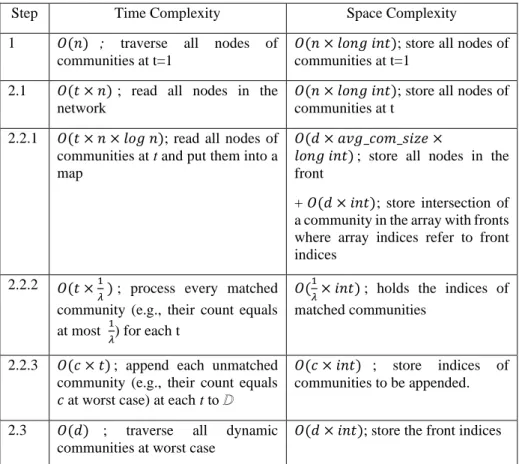
As it seen from Table 1, the most time-consuming task in this method is building and filling a map for tracking the place of each node in the fronts in Step 2.2.1 for preparation of matching process. Note that traversing nodes for each time step takes at most 𝑂(𝑡 × 𝑛) computation time and adding them into a map requires at most 𝑂(𝑙𝑜𝑔 𝑛) computation time. Therefore, time complexity of the method is 𝑂(𝑡 × 𝑛 × 𝑙𝑜𝑔 𝑛 ); in overall. The most space-consuming steps are Step 2.1. and Step 2.2.1. Therefore, the method needs memory space as 𝑂(𝑛 + (𝑑 × 𝑎𝑣𝑔_𝑐𝑜𝑚_𝑠𝑖𝑧𝑒) × 𝑙𝑜𝑛𝑔) type for storing nodes at each time step and nodes at front communities.

Fig. 1.A pseudocode for Greene et al.’s method Table 1. Complexity values of each step at pseudocode in Fig. 1.

Step Time Complexity Space Complexity

1 𝑂(𝑛) ; traverse all nodes of communities at t=1

𝑂(𝑛 × 𝑙𝑜𝑛𝑔 𝑖𝑛𝑡); store all nodes of communities at t=1

2.1 𝑂(𝑡 × 𝑛) ; read all nodes in the network

𝑂(𝑛 × 𝑙𝑜𝑛𝑔 𝑖𝑛𝑡); store all nodes of communities at t

2.2.1 𝑂(𝑡 × 𝑛 × 𝑙𝑜𝑔 𝑛); read all nodes of communities at t and put them into a map

𝑂(𝑑 × 𝑎𝑣𝑔_𝑐𝑜𝑚_𝑠𝑖𝑧𝑒 ×

𝑙𝑜𝑛𝑔 𝑖𝑛𝑡) ; store all nodes in the front

+ 𝑂(𝑑 × 𝑖𝑛𝑡); store intersection of a community in the array with fronts where array indices refer to front indices

2.2.2 _{𝑂(𝑡 ×}1

𝜆 ) ; process every matched

community (e.g., their count equals at most 1

𝜆) for each t

𝑂(1

𝜆× 𝑖𝑛𝑡) ; holds the indices of

matched communities

2.2.3 𝑂(𝑐 × 𝑡) ; append each unmatched community (e.g., their count equals 𝑐 at worst case) at each t to ⅅ

𝑂(𝑐 × 𝑖𝑛𝑡) ; store indices of communities to be appended.

2.3 𝑂(𝑑) ; traverse all dynamic communities at worst case

Tajeuna et al.’s Method. A pseudocode for the method is shown in Fig. 2. The authors first build a binary matrix(A) between nodes and communities to represent memberships of nodes at Step 1. They create a Burt matrix(B) where 𝐵 = 𝐴𝑇_{× 𝐴 to}

define the number of common nodes between communities in Step 2; keeping mind we use Eigen library residing http://eigen.tuxfamily.org website for fast matrix multiplication. They transform B into a transition matrix to calculate the transition probabilities between communities by normalizing entries of B in Step 3. They track communities in Step 4. For this reason, they hold a set S and initialize S with currently tracked community (𝐶𝑖) to hold evolution chain of at Step 4.1. They check mutual

transition (e.g. sim()) between each community with most recent time (𝑡𝑥) in S(𝐶𝑡𝑘_𝑥)and

each community at time step 𝑡𝑗(𝐶𝑡𝑗

𝑚_{) and check Jaccard similarity(JS) between 𝐶} 𝑡𝑗

𝑚 _and

𝐶𝑖. If both mutual transition and JS is greater than the similarity threshold 𝜆, 𝐶𝑡𝑗

𝑚 _is

added to evolution chain, S at Step 4.2.1.1. Mutual transition between two communities is sum of harmonic means of each entries of correspondent transition matrix rows. Jaccard similarity is directly computed correspondent entries of normalized Burt matrix.

Fig. 2.A pseudocode of Tajeuna et al.’s method

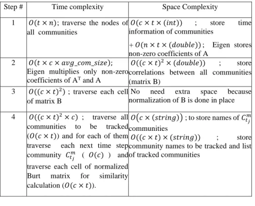
In Table 2, complexity values of each step in Fig. 2 are seen. Specifically, the most time-consuming task is similarity calculation between tracked communities and prospective next time step communities at Step 4.2.1.1. This calculation is done for all communities at next time step (𝑂(𝑐)) for each tracked community (𝑂(𝑐 × 𝑡)) and the similarity calculation cost between two community is 𝑂(𝑐 × 𝑡). Therefore, the running time complexity of the method is 𝑂((𝑐 × 𝑡)2_{× 𝑐). The space complexity of the work}

Table 2. Complexity values of each step at pseudocode in Fig. 2.

Step # Time complexity Space Complexity

1 𝑂(𝑡 × 𝑛); traverse the nodes of all communities 𝑂(𝑐 × 𝑡 × (𝑖𝑛𝑡)) ; store time information of communities +𝑂(𝑛 × 𝑡 × (𝑑𝑜𝑢𝑏𝑙𝑒)) ; Eigen stores non-zero coefficients of A 2 𝑂(𝑡 × 𝑐 × 𝑎𝑣𝑔_𝑐𝑜𝑚_𝑠𝑖𝑧𝑒); Eigen multiplies only non-zero coefficients of AT _{and A}

𝑂((𝑐 × 𝑡)2_{× (𝑑𝑜𝑢𝑏𝑙𝑒)) ; store}

correlations between all communities (matrix B)

3 𝑂((𝑐 × 𝑡)2_{) ; traverse each cell}

of matrix B

No need extra space because normalization of B is done in place 4 𝑂((𝑐 × 𝑡)2_{× 𝑐) ; traverse all}

communities to be tracked (𝑂(𝑐 × 𝑡)) and for each of them traverse each next time step community 𝐶𝑡𝑚_𝑗 ( 𝑂(𝑐) ) and

traverse each cell of normalized Burt matrix for similarity calculation (𝑂(𝑐 × 𝑡)).

𝑂(𝑐 × (𝑠𝑡𝑟𝑖𝑛𝑔)) ; to store names of 𝐶𝑡𝑚_𝑗

communities

𝑂((𝑐 × 𝑡) × (𝑠𝑡𝑟𝑖𝑛𝑔)) ; store community names to be tracked and list of tracked communities

3

Experiments & Results

3.1 Data Sets, Assumptions and Environment for Experiments

In this section, we test Greene et al.’s method and Tajeuna et al.’s method on a dynamic benchmark dataset. This dataset is generated by Greene et al. The dataset is constructed from four different synthetic graphs where each of them contains five static networks (e.g., five time steps) with 15000 nodes to simulate nonconsecutively evolving communities and includes six different community evolution events such as birth, death, growing, shrinking, merge and split. The dataset can be found online at http://mlg.ucd.ie/dynamic.

• The ‘Intermittent’ dataset contains the nonconsecutively evolving communities. • The ‘BirthDeath’ dataset is created to simulate form and dissolution of communities.

Greene et al. create birth of 40 additional communities by transferring nodes of other existing communities and randomly remove 40 existing communities along the network.

• The ‘ExpandContraction’ dataset is created to simulate growing and shrinking of communities. Greene et al. make growing and shrinking for randomly chosen 40 communities by 25% of their previous sizes.

• The ‘MergeSplit’ dataset is created to simulate merge of two existing communities and splitting of an existing community into two new communities. Greene et al. introduce 40 split and 40 merge events.

We design the following experiment to compare their accuracies and running speeds under the same conditions. For the equality of similar steps of both algorithms (e.g. detection of existing communities at each step); we use Louvain algorithm [11] and we remove the communities that have less than 3 nodes for both approaches. We download executable and source code of Greene et al.’s method [7] and use for experimental results. But, since neither source code nor executable of Tajeuna et al.’s method is open to public, we implement their method with same programming language (C++) with Greene et al.’s. We use a laptop with Core i7 2.30 GHz CPU and 8GB memory with our testbeds. Note that similarity threshold is taken as 0.1 for both methods because Greene et al. use this value in their experiment.

3.2 Results of Experiments

It is possible to evaluate the quality of detected communities by using Normalized Mutual Information (NMI) [12], if the ground-truth community information is already known. NMI measures accuracy of detected community structure by comparing them with the ground-truth structure and it produces a real value in [0,1]. The higher NMI values show that community detection done is better.The measurements are seen in Table 3 and Table 4 for each benchmark dataset.

The NMI values recorded in Table 3 are values with 92% accuracy rate. For the work of Tajeuna et al.[10], the NMI values reside in Table 4 with 98% accuracy rate. We calculate them via an NMI calculation software [13], by feeding of ground truth and detected community information for each step.

Table 3. NMI values for Greene et al.’s method[7] Time-steps BirthDeath NMI ExpandContraction NMI Intermittent NMI MergeSplit NMI t=1 0,88 0,88 0,88 0,88 t=2 0,93 0,94 0,91 0,94 t=3 0,92 0,93 0,94 0,92 t=4 0,92 0,96 0,93 0,91 t=5 0,94 0,96 0,92 0,88

In the light of accuracy values that we obtain, we can say that Tajeuna et al.’s method performs better than Greene et al.’s method in terms of accuracy.

Table 4. NMI values for Tajeuna et al.’s method[10] Timesteps BirthDeath NMI ExpandContraction NMI Intermittent NMI MergeSplit NMI t=1 0,996729 0,998628 0,99493 0,995583 t=2 0,995638 0,99618 0,987166 0,974798 t=3 0,995151 0,981107 0,98827 0,944636 t=4 0,991624 0,977629 0,992919 0,934176 t=5 0,994112 0,974361 0,989547 0,905201

4

Discussion of the Methods and Conclusion

Table 5. Overview of the methods

Capabilities Greene et al.’s method

(2010)

Tajeuna et al.’s method (2015)

1 Threshold setting Manually set Automatically set 2 Tracking Consecutive & partially

nonconsecutive

Consecutive &

nonconsecutive 3 Missing Event type Continue event type is

not defined.

All event types are defined.

4 Merge events Identification is limited to two communities.

There is no limitation. n communities can merge. 5 Split events A community can only

be split into two communities.

There is no limitation. A community can be split into

m communities 6 Space Complexity 𝑂(𝑛 + (𝑑 × 𝑎𝑣𝑔_𝑐𝑜𝑚_𝑠𝑖𝑧𝑒) × (𝑙𝑜𝑛𝑔)) 𝑂((𝑐 × 𝑡)2_{× (𝑑𝑜𝑢𝑏𝑙𝑒))} 7 Time Complexity 𝑂(𝑡 × 𝑛 × 𝑙𝑜𝑔 𝑛) 𝑂((𝑐 × 𝑡)2_{× 𝑐))} 8 Accuracy on the benchmark dataset 92 % 98%

In this study; we have presented a comparative study of two recent community tracking methods. Greene et al.’s method [7] is published in 2010 and Tajeuna et al.’s [10] method is published in 2015. Both methods focus on dynamically evolving data networks, to analyze their community relations on static and time sliced data pools. We test them on ground truth benchmark datasets in terms of accuracy and do their

complexity analysis. Hereunder, Table 5 summarizes a comparative analysis for selected criteria between both methods.

Criteria 1 & 2 & 3 & 4 & 5 are satisfied by Tajeuna et. al.’s method with higher accuracy. Threshold setting is automatically tuned according to the average number of nodes shared among all detected communities. Which is requirement overall high accuracy on continuing analyses among communities for long time series. Tracking of each community with all possible event types on non-consecutive time steps is important.

Criteria 6 & 7: Running times obtained from our experimental study are matched with time complexity analysis. Greene et. al.’s method should be preferred in very fast computation with predetermined similarity threshold requirement, but results are less accurate. On the other hand, Tajeuna et al.’s method should be preferred in the need of high accuracy and automatic similarity threshold requirements, but it needs high computation time with sufficient memory space.

In future, we will focus on tracking communities on real world networks and predicting community evolution events.

References

1. S. Lin, Q. Hu, G. Wang, and S. Y. Philip: Understanding community effects on information diffusion. pp. 82-95. In Proceedings of Pacific-Asia Conference on Knowledge Discovery and Data Mining(PAKDD), pp. 82-95, Springer, Ho Chi Minh City, Vietnam (2015) 2. D. A. Luke, and J. K. Harris: Network analysis in public health: history, methods, and

applications. Annu. Rev. Public Health 28, 69-93(2007)

3. A. Calvó‐Armengol, and Y. Zenou: Social networks and crime decisions: The role of social structure in facilitating delinquent behavior. International Economic Review 45(3), 939-958(2004)

4. D. Kempe, J. Kleinberg, and É. Tardos: Maximizing the spread of influence through a social network. pp. 137-146. In Proceedings of the ninth ACM SIGKDD international conference on Knowledge discovery and data mining, pp. 137-146, ACM, Washington DC, USA(2003) 5. M. Zanin, P. Cano, J. M. Buldú, and O. Celma: Complex networks in recommendation systems. pp 120-124. In Proceedings of second International Conference on Computer Engineering and Applications, World Scientific Advanced Series In Electrical And Computer Engineering(WSEAS), pp 120-124, Acapulco, Mexico(2008)

6. Z. He, E. G. Tajeuna, S. Wang, and M. Bouguessa: A Comparative Study of Different Approaches for Tracking Communities in Evolving Social Networks. pp. 89-98. In Proceedings of 2017 IEEE International Conference on Data Science and Advanced Analytics (DSAA), pp 89-98, Tokyo, Japan(2017)

7. D. Greene, D. Doyle and P. Cunningham: Tracking the evolution of communities in dynamic social networks. pp. 176-183. In Proceedings of International conference on Advances in social networks analysis and mining (ASONAM), pp. 176-183,IEEE,Odense, Denmark(2010)

8. M. Takaffoli, J. Fagnan, F. Sangi, and O. R. Za¨ıane: Tracking changes in dynamic information networks. Pp 94-101. In Proceedings of International Conference on Computational Aspects of Social Networks (CASoN), pp. 94–101, Salamanca, Spain(2011) 9. P. Brodka, S. Saganowski, and P. Kazienko: Ged: the method for group evolution discovery

in social networks. Social Network Analysis and Mining 3(1), 1–14(2013)

10. E. G. Tajeuna, M. Bouguessa, and S. Wang: Tracking the evolution of community structures in time-evolving social networks. pp 1-10. In Proceedings of International Conference on Data Science and Advanced Analytics (DSAA), pp. 1–10, Paris, France(2015)

11. V. D. Blondel, J.-L. Guillaume, R. Lambiotte and E. Lefebvre E.:Fast unfolding of communities in large networks. Journal of statistical mechanics: theory and experiment 2008(10), 10008(2008)

12. L. Danon, A. Diaz-Guilera, J. Duch, and A. Arenas: Comparing community structure identification. Journal of Statistical Mechanics: Theory and Experiment 2005(09), P09008(2005)

13. A. Lancichinetti, S. Fortunato and J. Kertesz:Detecting the overlapping and hierarchical community structure in complex networks. New Journal of Physics, 11(3), 033015(2009)