Design and Implementation of a Negative Feedback Oscillator Circuit
Based on a Cellular Neural Network with an Opposite Sign Template
BARAN TANDER
1, ATİLLA ÖZMEN
2, YASİN ÖZCELEP
31
Electronic Communication Technology Program
Kadir Has University
Vocationary School of Technical Sciences, 34590 Silivri/İSTANBUL
TURKEY
[email protected]
2Department of Electronics Engineering
Kadir Has University
School of Engineering, 34083 Fatih/İSTANBUL
TURKEY
[email protected]
3Department of Electrical&Electronics Engineering
İstanbul University
School of Engineering, 34320 Avcılar/İSTANBUL
TURKEY.
[email protected]
Abstract: - In this paper, explicit amplitude and frequency expressions for a Cellular Neural Network with an Opposite-Sign Template (CNN-OST) under oscillation condition are derived and a novel inductorless oscillator circuit with negative feedbacks, based on this simple structure is designed and implemented. The system is capable of generating quasi-sine signals with tuneable amplitude and frequency which can’t be provided at the same time in the classical oscillator circuits.
Key-Words:
- Oscillator Circuits, Cellular Neural Networks, Quasi-Sine Signals, Curve and Surface Fitting, Operational Amplifiers, Circuit Design.1 Introduction
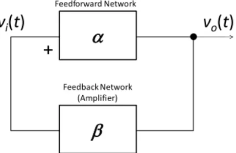
Oscillators are electronic circuits that produce periodical signals (sinusoids, square waves etc.), which play very important roles, especially in communication systems. Colpitts/Hartley, Phase-shift and Wien are widely used sinusoidal oscillator types [1]. The block diagram of a conventional sinusoidal oscillator is shown in Fig. 1.
a
b
Feedforward Network Feedback Network (Amplifier)v
o(t)
v
i(t)
+
Fig. 1: Block diagram of a
conventional sinusoidal oscillator.
Here, the vo(t) is the periodical output voltage, vi(t) is the feedback voltage.
) ( ) ( t v t v i o
a is the voltage gain
of the feedforward, ) ( ) ( t v t v o i
b is the voltage gain of
the feedback networks. The operation principle is as follows:
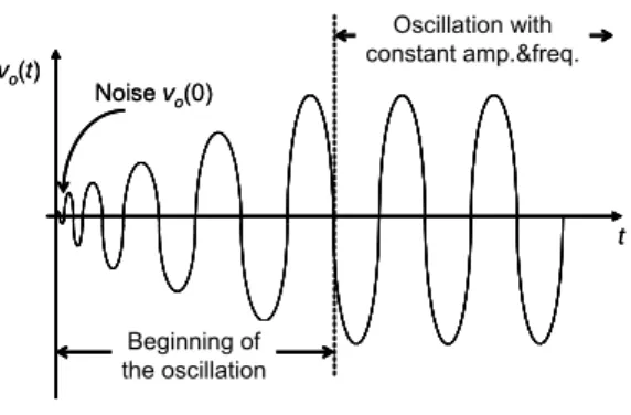
The noise in the medium which can be considered as the initial condition vo(0) for the output voltage, is captured and amplified by the feedforward block employing an active component such as a transistor
or an Operational Amplifier (OpAmp), while a 180o
phase shift is realized by the passive positive feedback network, until a periodical sine with constant amplitude and frequency is generated as shown in Fig. 2. The feedback network also sets the frequency of the output signal.
Fig. 2: Operation principle
of a sinusoidal oscillator.
The oscillation constraint is strict (
a
b
1)and is determined by voltage gains of both blocks. It can be set to a greater value, however in this case the active component at the feedforward network will saturate. Therefore, the amplitude of oscillation depends only to the source voltage of the active component. Despite the system proposed in this paper, in classical oscillators, the tuning of the amplitude by varying the values of circuit components is not possible because of the positive feedback.Papers about negative feedback oscillators also exist in literature [2], however our system depends on a Cellular Neural Network (CNN) architecture, therefore having a simpler design, since it only contains fundamental OpAmp application blocks. The paper is organized as follows; first, a brief information about the CNNs are given and a special CNN system, CNN-OST and its oscillation constraint are introduced. The amplitude and frequency surfaces with respect to template elements are sketched and two explicit analytical approaches are found for each. Secondly, a circuit based on this simple topology is designed, simulated and implemented. The output voltages are compared with the numerical solutions of the nonlinear differential equation system defining the structure. Finally, the advantages and drawbacks of the proposed circuit and future works that can be done are discussed.
2
CNNs
2.1.
CNNs and Their Applications
CNNs are a class of dynamical neural networks and were first proposed by Chua and Yang [3] which
find very effective applications in image processing [4], as well as in chaotic signal generation because of their nonlinear manner [5]. The block diagram of a CNN neuron (cell) is sketched in Fig. 3.
Fig. 3: Block diagram of a CNN cell.
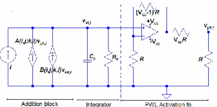
As a dynamic neural network, CNN cells include an integration unit, however unlike the Hopfield nets, here, cells only interact with each other by the r neighbourhood definition given below:
C k i l j r k M l N
Nij klmax , ;1 ,1 (1)
According to (1), at a neighbourhood dimension of r = 1, a cell will only interact with its nearest neighbours. This constraint will dramatically decrease the number of weight coefficients between cells Cij and Ckl at an MxN-cell system, enabling a simple implementation. The nonlinear differential equation for a CNN cell C(i,j) shown in Fig. 3 is given by, I u l k j i B y l k j i A x xi,j i,j (, ; , ) k,l (, ; , ) k,l (2) Where xi,j is the “state” of the cell C(i, j) which we will mostly deal throughout the paper; yk,l is the “output”, uk,l is the “input” of its neighbour C(k,l); A(i, j; k l) is the “weight coefficient” between C(i, j) and the output of C(k,l); B(i,j;k,l) is another “weight coefficient” between C(i, j) and the input of C(k,l); and finally, I is a “threshold” value common for all cells. The activation function namely, “Piecewise Linear Function” (PWL) shown in Fig. 4 can be written as follows
1
1
2
1
, , ,j
i j
ij
ix
x
y
(3) vo(t) t Beginning of the oscillation Oscillation with constant amp.&freq. Noise vo(0) vo(t) t Beginning of the oscillation Beginning of the oscillation Oscillation with constant amp.&freq. Oscillation with constant amp.&freq. Noise vo(0)Fig. 4: The PWL activation function of a
CNN cell.
The circuit model of the cell C(i,j) is given in Fig. 5. Here, the vxi,j is the “state” xi,j; vyi,j is the “output” yi,j; A(i,j;k,l) and B(i,j;k,l) are the “weight coefficients” between the cells C(i,j) and C(k,l). The voltage controlled current sources that can easily be realized by OpAmp blocks, and the cascaded non-inverting amplifier and voltage divider at the output providing the PWL activation function, will be discussed at Section 3.1 in detail.
Fig. 5: Circuit model of a CNN cell.
2.2. CNN-OST
Although large number of cells are employed in image processing applications with CNNs [6], a simple version of these networks CNN-OST [7], introduced by Zou and Nossek including only two neurons as seen in Fig. 6 can be used as an oscillator.
Fig. 6: CNN-OST.
The nonlinear differential equations written in matrix form that define the system is given below:
0 , 0 ; ) ( ) ( 2 1 2 1 2 1 b a a b b a x y x y x x x x A (4)
Here A is the template matrix that contains the weight coefficients. The a and b are, A(i,j;i,j) the self weight coefficient of a cell and A(i,j;k,l) the weight coefficient with its neighbor, respectively. As seen from (4), the system contains neither B(i,j;k,l) nor I. The x1 and x2 solutions can be
considered as the outputs. Under oscillation conditions [8], they will have exactly the same amplitude and frequency, however with phase shifts, therefore analyzing only one of them will be sufficient [9].
3
Amplitude
and
Frequency
Surfaces
The variations in A change the stability of the system. Savacı and Vanderwelle proved that x1 and
x2 solutions are oscillations under the following
constraint [8]:
b > a - 1 (5)
The oscillations are in quasi-sine waveforms because of the nonlinear characteristic of the PWL activation function. The first goal is to assign explicit formulas for the amplitudes and frequencies of these oscillations with respect to the template components. This process is carried out by sketching the 3D surfaces as functions of as and bs under the constraint in (5). Mentioned graphics are shown in Fig. 7a and b. (a) yi,j 1 xi,j -1 1 -1 C(1,1) C(1,2) a -b b a A m plit ude A m plit ude
(b)
Fig. 7: (a) a and b,
(b) Change of frequency with a and b, under the constraint given in (5).
As seen from Fig. 7a, the amplitude depends on a and is independent from b, specifically, linearly increasing with a, therefore can be expressed with the form below:
G(a)=Aa+B (6)
It is clear that, this enables the tuning of the G(a) amplitude by changing the avalues. The following A and B coefficients are found by utilizing curve fitting methods within the limitations chosen for the mesh plot:
A=2.0013 (7a)
B=-0.8332 (7b)
One can see that by analyzing the graphic in Fig. 7b, the frequencies of the oscillations depend on
both aand bvalues. Therefore the following
analytical approach will be convinient to describe the dealed parameter:
F(ab)=(C/a)b+D(a) (8)
Here, the D(a) function is a polynomial with a chosen order of seven which is found by trial and error as the optimum. After a surface fitting process
for Fig. 7b, the numerical values for C and the D(a)
polynomial are determined as:
C=0.14 (9a)
D(a)=-1.2651+2.8768a-2.5932a2+1.2839a3 -0.3961a4+0.0812a5-0.0115a6+0.0011a7 (9b)
These analytical approaches prove that, both amplitudes and frequencies of the signals generated by the system are controllable unlike the conventional oscillators. In order to find the template component values for a chosen amplitude and frequency pair, one must solve the two nonlinear equations (6) and (8) for a and b.
3.
Oscillator Circuit Based on
CNN-OST
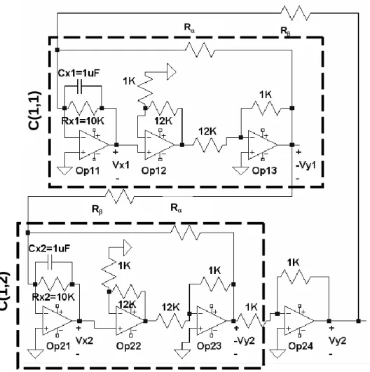
3.1
Circuit Design
The topology proposed in Fig. 8 is suitable for the realization of the equation system that defines the
CNN-OST, where the a and b components are
represented by the conductances of the Raand Rb
resistors between the cells [10,11]. The circuit will
generate quasi-sine signals under specific
component values, however without employing positive feedbacks seen in the conventional oscillator circuits, since all the feedbacks are applied to inverting-inputs of the OpAmps as seen from the
schematic. The resistances simulating the
components can be computed as follows:
a a Rx R (10a) b b Rx R (10b)
The node-voltage-equation for the inverting input of the OpAmp Op11 at cell C(1,1), can be written as in (11), if the OpAmp is assumed to be ideal where vx1 is the state of this cell, vy1 is its output and vy2 is the output of the neighbouring cell.
1 1 2
1 1 y y x x x x v v v C R v a b (11)It is clear that by choosing 1/RxCx = 1, the above equation becomes the first row of (4). Here, the Op12-Op13 and Op22-Op23 inverting and
non-inverting amplifier pairs provide the PWL
characteristics of the activation functions for both cells. In order to obtain the negative b value in (4), an extra inverting amplifier circuitry (Op24) with a gain of “-1” is attached at the output of the cell C(1,2). The quasi-sine oscillations are the vx1 and vx2 “states” taken from the outputs of the OpAmps Op11 and Op21 providing the load independency as well, since the input resistances of the OpAmps can be assumed as open-circuits. F re qu en cy F re qu en cy
Fig. 8: Proposed oscillator circuit.
3.2.
Frequency Denormalization
The 1/RxCx coefficient at (11) determines the range of the oscillations’ frequency. Specifically, as 1/RxCx increases the frequency band will increase and decrease vice-versa [12]. By varying either Rx or Cx values, a denormalization process can be carried out by the multiplication of the right hand side of the equation, with the frequency therefore, it is possible to generate oscillations on a wide frequency range without ever changing the resistors for a and b. It is better to vary Cx instead of Rx to achieve this purpose otherwise, as seen from (10), Ra and Rb
therefore the mentioned components will be changed for varied Rx values.
One can use stereopotentiometers in order to adjust the values of as and bs simultaneously, to set the desired amplitude and frequency.
4
Simulation and Implementation
In this section, first, an analysis is performed for a chosen Ra and Rb pair, by comparing the theoretical
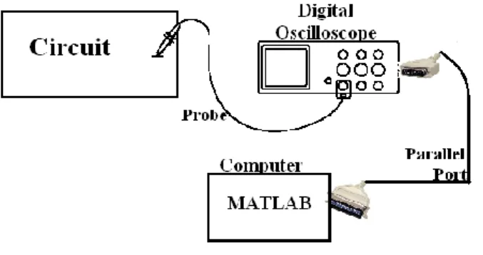
values of the amplitude and frequency computed by the numerical solutions of (6) and (8) by using a 2-cell CNN model constructed in MatLab Simulink software given in Fig. 9 [11], with the ones obtained from the simulated and implemented circuits. Here, the A and B coefficients in the state equation blocks correspond to 1/RxCx , and the K gains denote the as and bs between the cells, furthermore Cs and Ds must be chosen as 1 in this model. The PSpice software is used for the circuit simulations. The measurement set up for the implementation is given in Fig. 10.
Then as a synthesis procedure, for a specific amplitude and frequency pair, the design is verified by comparing the measured outputs of the oscillator circuit with the simulation as well as with the numerical solutions of (6) and (8). As depicted
Ra Rb Ra Rb
C(1,1
)
C
(1,2
)
Ra Rb Ra Rb Ra Rb Ra RbC(1,1
)
C
(1,2
)
Ra Rbbefore, the two components of the state set, vx1 and
vx2, have exactly the same characteristic and
waveform however with phase shifts, therefore analyzing a single state (vx1) is enough.
Fig. 9: The Simulink Model for the CNN based
oscillator.
Fig. 10: The measurement set up for
implementation.
4.1. Analysis
If standard resistors Ra=2.2k, Rb=470 and
Rx=10k are chosen, a and b become 4.545 and
21.276 respectively from (10). Then, by using the analytical approaches given in (6) and (8), the amplitudes and frequencies of the oscillations are computed as, G=7.918V and f=0.625Hz with the model given in Fig. 9. Here, the Cx value is chosen as 1μF, which will denormalize the frequency by
1/RxCx=100 and change it to 62.500Hz as depicted in
Section 3.2, for the ease of monitoring the
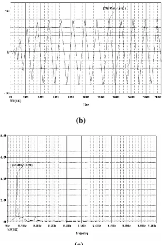
oscillations with a standard oscilloscope. The piecewise activation relationship between the state and the output of the cell C(1,2) is given in Fig. 12a. The numerical, simulation and implementation results are given in Fig. 11, 12 and 13, respectively.
0 0.02 0.04 0.06 0.08 0.1 0.12 0.14 0.16 0.18 0.2 -10 -8 -6 -4 -2 0 2 4 6 8 10 Time(sec) O u tp u t V o lt a g e (V ) (a) 0 50 100 150 200 250 300 350 400 450 500 0 100 200 300 400 500 600 700 Frequency(Hz) ff t o f th e s ig n a l (b)
Fig. 11: The numerical results for the analysis
process by using the model given in Fig. 9. (a) Time domain simulation, (b) Frequency domain simulation.
(a) XY Graph x' = Ax+Bu y = Cx+Du State-Space1 x' = Ax+Bu y = Cx+Du State-Space Saturation1 Saturation -K-Gain4 -K-Gain3 -K-Gain2 -K- Gain1 Clock
(b)
(c)
Fig. 12: Circuit simulations for analysis process: (a) The simulation of the piecewise linear activation
function at cell C(1,2)
(b) Time-domain simulation, (c) Frequency domain simulation
for the analysis process when Ra =2.2k, Rb=470.
(a)
(b)
Fig. 13: (a) Implementation result in time domain, (b) In frequency domain when
Ra =2.2k, Rb=470 by using the set up in Fig. 10.
4.2. Synthesis
Here, the amplitude is chosen as G=12V and the frequency as f=1Hz. By solving (6) and (8) simultenously, the a and b values are found as 6.410
and 47.030, which make the corresponding
interconnected resistances Ra and Rb 1560.062
and 212.630 respectively according to (10).
Standard resistors 1500 and 220 are employed in
the simulation and implementation. Moreover, the
1/RxCx coefficient is made 100 again by choosing
Rx=10k and Cx=1μF which will denormalize the
oscillation frequency to 100Hz. Numerical,
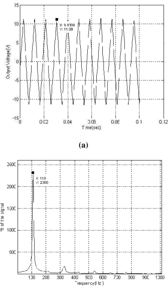
simulation and implementation results in time and frequency domains results are sketched in Fig. 14, 15 and 16. 0 0.02 0.04 0.06 0.08 0.1 0.12 0.14 0.16 0.18 0.2 -15 -10 -5 0 5 10 15 Time(sec) O u tp u t V o lt a g e (V ) (a)
0 50 100 150 200 250 300 350 400 450 500 0 1000 2000 3000 4000 5000 6000 7000 8000 9000 Frequency(Hz) ff t o f th e s ig n a l (b)
Fig. 14: The numerical results at the synthesis
process by using the model given in Fig. 9.
(a) Time domain simulation, (b) Frequency domain simulation.
(a)
(b)
Fig. 15: Circuit simulations for synthesis process: (a) Time-domain simulation,
(b)Frequency domain simulation for chosen
amplitude of 12V and frequency of 100Hz
(a)
(b)
Fig. 16: (a) Implementation result in time domain, (b) In frequency domain for chosen amplitude of
12V and frequency of 100Hz.
Since the oscillations are quasi-sines, one can see that by analyzing all of the frequency domain results, the peak value of the amplitude is not exactly equal to the desired value because of the effect of side harmonics. However, as seen from the operations in time domain, the amplitudes of the oscillations take satisfactory values pretty close to the proposed ones.
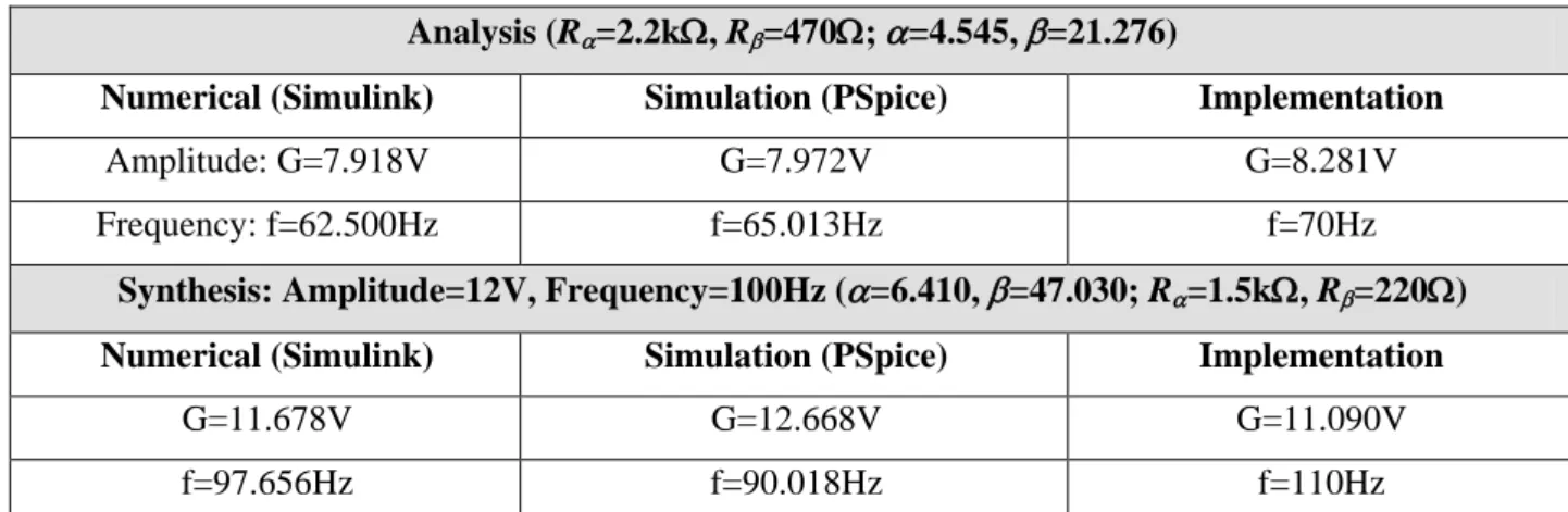
Results of the numerical computations, simulations and implementations are summarized in Table-I.
5
Conclusions
In this paper, a CNN based oscillator circuit is designed and implemented. Unlike the classical oscillators, the proposed circuit has negative
Table - I: Summary of numerical, simulation and implementation results for analysis and synthesis processes.
Analysis (Ra=2.2k, Rb=470; a=4.545, b=21.276)
Numerical (Simulink) Simulation (PSpice) Implementation
Amplitude: G=7.918V G=7.972V G=8.281V
Frequency: f=62.500Hz f=65.013Hz f=70Hz
Synthesis: Amplitude=12V, Frequency=100Hz (a=6.410, b=47.030; Ra=1.5k, Rb=220) Numerical (Simulink) Simulation (PSpice) Implementation
G=11.678V G=12.668V G=11.090V
f=97.656Hz f=90.018Hz f=110Hz
feedbacks and tuneable amplitude. Since it is based on a 1x2-cell structure CNN-OST, it is capable of generating two quasi-sine signals at the same time with phase shifts. Furthermore, the design is inductorless.
The classical 741 BJT OpAmp ICs are employed in the simulation and implementation. If high performance FET OpAmps are used, it is obvious that even more accurate results can be obtained. Having too many components when compared to conventional oscillators is a drawback, it also seen that the closer the a and b values the worse the output wave shape which must be taken into account in the design. Moreover, because of the nonlinear activation function at the CNN cells, the outputs are not exact sinewaves, therefore contains side harmonics, however, the design is believed to be employed in many applications and suitable for integration.
References:
[1] Boylestad R., Nashelsky L., Electronic
Devices and Circuit Theory 5th Ed., Prentice Hall International Inc., 1992,
[2] Wang R., Jing Z., Chen L., Periodic
Oscillators in Genetic Networks with Negative Feedback Loops, WSEAS Trans. on Mathematics, Vol. 3, No. 1, 2004, pp. 150-157,
[3] Chua L.O., Yang L., Cellular Neural
Networks: Theory, IEEE Trans. CAS, Vol. 35, No. 10, 1988, pp. 1257–1272,
[4] Costantini G., Casali D., Carota M.,
Detection of Moving Objects in 2-D Images Based on a CNN Algorithm and Density Based Spatial Clustering, WSEAS Trans. on Circuits and Systems, Vol. 4, No. 5, 2005, pp. 440-447,
[5] Aissi C., Kazakos D., An Autonoumous
Chaotic CNN Hysteresis Circuit, WSEAS Trans. on Systems, Vol. 3, No. 1, 2004, pp. 216–220,
[6] Amanatidis D., Tsaptsinos D., Giaccone
P.R., Jones G.A., Image Processing Using
CNNs and FPGAs: Initial Results,
NNA2001: WSES International Conference on Neural Network and Applications, Tenerife, Spain, 2001,
[7] Zou F., Nossek J.A., Stability of Cellular
Neural Networks with Opposite-Sign
Templates, IEEE Trans. CAS, Vol. 38, No. 6, 1991, pp. 675–677,
[8] Savaci F.A., Vanderwalle J., On the
Stability of Cellular Neural Networks, IEEE Trans. CAS– I: Fund. Theo. and Apps., Vol. 40, No. 3, 1993, pp. 213–215,
[9] Özmen A., Tander B., A Numerical Method
For Frequency Determinatıon in the Astable Cellular Neural Networks with Opposite-Sign Templates, SIU’06: 14th IEEE Opposite-Signal
Processing and Communication
Applications Conference, Antalya, Turkey, 2006, (In Turkish),
[10] Tander B., Özmen A., Analytical
Approaches for the Amplitude and
Frequency Computations in The Astable Cellular Neural Networks With Opposite-Sign Templates, SIU’07: 15th IEEE Opposite-Signal
Processing and Communication
Applications Symposium, Eskişehir, Turkey, 2007, (In Turkish),
[11] Tander B., Ün M., Generalized PSPICE and
SIMULINK Models for the Continious-Time Simulations of Cellular Neural
Networks, BCSP’2000, 1st IEEE Balkan
Conference on Signal Processing,
Communications, Circuits and Systems, Istanbul, Turkey, 2000,
[12] Tander B., Başkan M., Şenol C.,
Experimental Analysis of Transients in Low Dimensional Cellular Neural Networks, ELECO’02: 4th Electronics and Computer Engineering Symposium, Bursa, Turkey, 2002 (In Turkish).