A comparative study on indirect determination of degree of weathering of granites from some physical and strength parameters by two soft computing techniques

(1)

A comparative study on indirect determination of degree of

weathering of granites from some physical and strength

parameters by two soft computing techniques

C. Gokceoglu

a,

⁎, K. Zorlu

b

, S. Ceryan

c

, H.A. Nefeslioglu

d

a_{Department of Geological Engineering, Applied Geology Division, Hacettepe University, Beytepe Ankara 06800, Turkey} b

Department of Geological Engineering, Applied Geology Division, Mersin University, Ciftlikkoy Mersin, 33342, Turkey

c_{Department of Geological Engineering, Balikesir University, Balikesir, Turkey} d_{Department of Geological Research, 06800 Ankara, Turkey}

A R T I C L E D A T A

A B S T R A C T

Article history: Received 22 May 2008 Received in revised form 27 March 2009

Accepted 9 June 2009

Weathering has several adverse effects on the physical, mechanical and deformation characteristics of rock. However, when determining the weathering degree of rocks, some difficulties are encountered. Ideally, the weathering degree can be determined by simple test results and reliable prediction models. Considering this situation, the purpose of the present study is to construct simple and low cost weathering degree prediction models with two soft computing techniques, artificial neural networks and fuzzy inference systems. When developing these models, model results were tested against data from specimens collected from the Harsit granitoid (NE Turkey) and data published in the literature. Model inputs are porosity, P-wave velocity and uniaxial compressive strength, and model output is weathering degree. The models developed in this study exhibited high prediction performances when checked by train and test data sets. This result shows that the models developed herein can be used for indirect determination of weathering degree. The artificial neural network model requests numerical data as the input, while the fuzzy inference system model can take numerical data and expert opinion as the input. As a conclusion, the models have a high potential when determining weathering degree of a rock for various purposes.

Granite Weathering

Artificial neural network Fuzzy inference system

1. Introduction

For a long time, weathering has been one of the major research areas of engineering geology and rock mechanics because weathering has an adverse influence on rock strength and deformability characteristics which in turn influences the industrial use of rocks. The properties of rock material are

controlled by the mineral composition, texture, fabric and the weathering state [1]. Almost all engineering projects are carried out at the surface of the earth or at a relatively shallow depth below the surface. This shallow domain is also the zone in which the processes of weathering, erosion and deposition are generally active[2]. For this reason, the correct description of weathered intact rock is required to predict its engineering

⁎ Corresponding author. Tel.: +90 312 2977735; fax: +90 312 2992034. E-mail address:cgokce@hacettepe.edu.tr(C. Gokceoglu).

a va i l a b l e a t w w w. s c i e n c e d i r e c t . c o m

(2)

behavior. ISRM [3] suggested a descriptive classification scheme for the weathering degree of intact rock material, but correct description requires extensive testing and difficul-ties may be encountered when applying this or other descriptive classification schemes.

In the last three decades, various researchers have attempted to obtain weathering degree using simpler and more reliable methods. The weathering degree classification processes can be divided into a qualitative or quantitative approach. Qualitative classification schemes are based on observational descriptions and simple index properties. These are color change[4], chemical weathering degree of feldspars or biotites[1,4–7], and observational description of physical weathering degree[3,7,8]. However, application of qualitative approaches is simple and easy to carry out in field, but may lead to inconsistent classification, because these include some subjective aspects.

Quantitative approaches lead to consistent and objective material descriptions more than qualitative approaches, particu-larly by non-specialist users [1]. Quantitative classification schemes may consider mineralogical properties, index proper-ties, or strength characteristics. Various mineralogical indices have been proposed (for ex.[9–14]), but changes in these indices may be affected by more than weathering alone. Differentiation in microcrack density can be controlled by parent rock mineralogy, local tectonic activity, or the technique used for preparation of thin-sections. Other quantitative weathering classification schemes consider some index or strength properties of rocks

[15–20]. According to Gupta and Rao[16], weathering produces gradational changes in the physico-chemical and mechanical properties of rocks and, ideally, this would be assessed in quantitative rather than qualitative terms. All of these studies have provided important contributions to the classification of weathering degree of intact rock material. However, determina-tion of weathering degree by a simple and reliable way is still open to development.

The main purpose of the present study is to construct predictive models for reliable estimation of weathering degree of granitic rocks using the two soft computing techniques, fuzzy inference system and artificial neural networks. For this purpose, samples from the Harsit granitoid (NE Turkey) were collected and the necessary descriptions and tests were performed. By using the data obtained from these descriptions and tests, two prediction models were constructed, and the models were then checked against the data in the literature.

2. Field and Laboratory Studies

Performed on the Harsit Granitoid

The Harsit granitoid crops out between Dogankent (Giresun) and Kurtun (Gumushane) in the northern zone of the Pontides (NE, Turkey) (Fig. 1). Field observations and sampling proce-dure were applied in this area. The younger formations in the sampling area are cross cut by the Harsit granitoid. Quartz diorite, quartz monzonite, quartz monzodiorite and leucogra-nite exist in the contrast zones of the batholith while the center of the Harsit pluton is formed by granodiorite[21]. All these granitic rocks intruded into the eastern Pontide volcanic arc during the period of Upper Cretaceous to Eocene[22,23].

The first stage of the study was to determine the weathering zones in the area. The selected profiles typically show weath-ering state changes gradually in the vertical section. To provide a representative sampling, samples with different degrees of weathering were collected from more or less uniform zones. The weathering classes of the rock material were determined by using the weathering classification suggested by[3]. The residual soils do not have their original volume due to frame collapse. Considering this problem, no sample was collected from the residual soil parts in the weathering profiles of the Harsit granitic rocks. A total of 32 block samples were collected, each with the approximate dimensions 30 × 30 × 30 cm3_{. Core}

samples from each weathering class were tested to determine various physical and mechanical properties such as unit weight, porosity, Schmidt hardness, P-wave velocity, point load index and uniaxial compressive strength. All core speci-mens were extracted in the vertical orientation. To provide standardization, the uniaxial compressive strength and P-wave velocity tests were applied on the air-dried core speci-mens extracted from a vertical direction. The uniaxial com-pressive strength tests on core specimens were performed using a standard stiff compression-testing machine. Physical and index properties, P-wave velocity and uniaxial compres-sive strength were determined during the laboratory testing

program in accordance with the procedure suggested by [3]

(Table 1). However, extracting standard core specimens from the completely weathered blocks for the uniaxial compressive strength tests was not possible. For this reason, some cubic

specimens having 5 × 5 cm2 _{dimensions were prepared and}

these tests were applied on the cubic specimens obtained from the completely weathered blocks. The unit weight values of the fresh samples are around 26.3 kN/m3_{while that of completely}

weathered samples decrease to 22.8 kN/m3. When applying

the point load index and Schmidt hammer tests on highly or completely weathered specimens, some serious difficulties were encountered. The Schmidt hammer test is one of the easiest tests to perform in rock mechanics. However, this test did not yield reasonable results when applied to highly weathered samples, especially completely weathered sam-ples. Due to this difficulty, the Schmidt hammer test results could not be used as an input for the prediction models. Another easy-to-perform test is the point load index, but similar difficulties were encountered so again the test results could not be used as an input. Changes for all weathering classes except residual soil could be measured during the porosity, unit weight, P-wave velocity and uniaxial compres-sive strength tests (Table 1).

Data for the model inputs should be easy to acquire. This is only possible if the models' inputs are the results of easy-to-perform tests. The porosity values of the specimens were calculated using the specific gravity and the dry density. The porosity values of the fresh samples varied between 1.4% and 3.7% while those of the completely weathered samples reached 19.5%, thus porosity was accepted as an indicator of the weathering degree and model input. The results of the tests on velocity of elastic waves and uniaxial compressive strength were directly dependent on degree of weathering, so the results may be used as model inputs. Although some difficulties have been encountered when preparing test specimens from the completely weathered blocks for P-wave

(3)

velocity and uniaxial compressive strength tests, the results of these tests are highly characteristic for the indirect determi-nation of the weathering degree of the granitic rocks. For these reasons, porosity, P-wave velocity and uniaxial compressive strength were selected as the inputs of the weathering degree prediction models.

A total of 32 cases including degree of weathering, porosity, P-wave velocity and uniaxial compressive strength were used for constructing prediction models. Before constructing the models, to apply a learning stage independent from magni-tude of data and to provide standardization among the inputs and the outputs, all data were normalized by using the following equations due to its simplicity (Eq. (1)):

Xn= Xi=Xmax ð1Þ

where, Xnis the normalized parameter; Xi is the measured

parameter and Xmaxis the maximum value of the X parameter

data set.

The normalization process may increase the usability of the models because the models will be independent from the magnitude of data. The normalization parameters (Xmax) are 5

for the weathering degree, 21.4 for the porosity, 4285 for the P-wave velocity and 167.9 for the uniaxial compressive strength. As seen fromTable 1, the degree of weathering leads to an increase in the average porosity value. Input parameter ranges, however, show an important overlap in weathering classes. In other words, it is impossible to determine the weathering class of a granite sample by employing only one absolute value of physical or engineering properties. The uniaxial compressive strength is proposed to be reliable as an index parameter, which consistently changes throughout the weathering spectrum. However, the direct use of unconfined compressive strength as an index parameter of weathering for common rocks is ineffective due to a high overlapping degree of given values[16].

A series of simple regression analysis between weathering degree and the selected input parameters such as porosity, P-wave velocity and uniaxial compressive strength was per-formed. A strong exponential relationship between the weathering degree and the porosity (Fig. 2a) is observed. On the other hand a moderate–strong inverse-linear relationship was observed between the weathering degree and the P-wave Fig. 1– Location map of the sampling area.

(4)

velocity (Fig. 2b). A strong inverse-exponential relationship between the weathering degree and the uniaxial compressive strength was also observed, which can be seen inFig. 2c. As mentioned before the overlapping can be clearly seen inFig. 2. These assessments revealed that estimating the weathering class of a granite sample by using the absolute value of only one parameter, is almost impossible which suggests that more than one input parameter is needed. Therefore, two prediction models with three inputs and an output were proposed. The data used for training was also used for checking to provide standardization between the models. 32 data obtained from the Harsit granitic rocks were used for training while a data set obtained from the literature[16]was employed as a checking data set (Table 2).

3. Artificial Neural Network Model

The application of artificial neural network (ANN) to rock mechanics and engineering geology has been presented

recently in the literature [24–27]. A neural network can be defined as a model of reasoning that is based on the way that the human brain functions[28]. The human brain comprises of densely interconnected sets of nerve cells, or basic information-processing units, called neurons. Considering its structure, the brain can be described as a highly complex, nonlinear and parallel information-processing system [28]. Subsequently, in fact an artificial neural network can be considered as a simplified reproduction or mirror of that highly complicated system. More than a hundred different types of artificial neural networks, new or modifications of existing ones can be encountered in recent literature[28–31]. Back propagation artificial neural networks are the most widely used type of networks[28]because of their flexibility and adaptability in modeling a wide spectrum of problems in many application areas[32].

When developing an artificial neural network, the data is partitioned into at least two subsets such as training and checking data. It is commonly expected that the training data include all the data belonging to the problem domain.

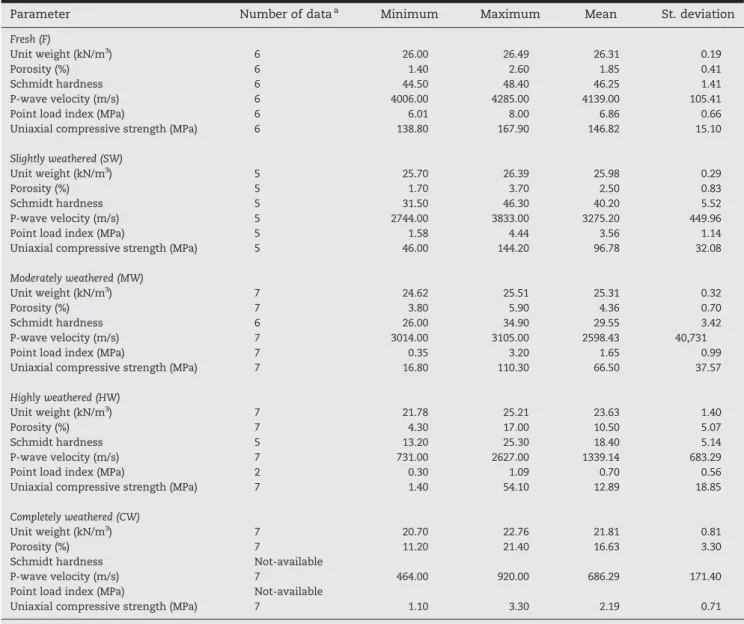
Table 1– Statistical assessments of the test results applied on the samples collected from the Harsit granitoid.

Parameter Number of dataa Minimum Maximum Mean St. deviation

Fresh (F)

Unit weight (kN/m3₎ ₆ _26.00 _26.49 _26.31 _0.19

Porosity (%) 6 1.40 2.60 1.85 0.41

Schmidt hardness 6 44.50 48.40 46.25 1.41

P-wave velocity (m/s) 6 4006.00 4285.00 4139.00 105.41

Point load index (MPa) 6 6.01 8.00 6.86 0.66

Uniaxial compressive strength (MPa) 6 138.80 167.90 146.82 15.10

Slightly weathered (SW)

Unit weight (kN/m3₎ ₅ _25.70 _26.39 _25.98 _0.29

Porosity (%) 5 1.70 3.70 2.50 0.83

Moderately weathered (MW)

Unit weight (kN/m3₎ ₇ _24.62 _25.51 _25.31 _0.32

Porosity (%) 7 3.80 5.90 4.36 0.70

P-wave velocity (m/s) 7 3014.00 3105.00 2598.43 40,731

Highly weathered (HW)

Unit weight (kN/m3₎ ₇ _21.78 _25.21 _23.63 _1.40

Porosity (%) 7 4.30 17.00 10.50 5.07

Completely weathered (CW)

Unit weight (kN/m3₎ ₇ _20.70 _22.76 _21.81 _0.81

Porosity (%) 7 11.20 21.40 16.63 3.30

Schmidt hardness Not-available

Point load index (MPa) Not-available

(5)

Certainly, this subset is used in the training stage of the model development to update the weights of the network. On the other hand, the check data should be different from those used in the training stage. The main purpose of this subset is to check the network performance using untrained data, and

to confirm its accuracy. No exact mathematical rule to determine the required minimum size of these subsets exists. However, some suggestions for these sampling strategies are encountered in literature [32]. These studies suggest that approximately 80% of entire data is common enough to train the network, and the rest is usually handled to check the final architecture of the model [33,34]. In this study, only one artificial neural network model was constructed to estimate the weathering degree of the Harsit granitoid. The input of the model is constituted of porosity parameters, P-wave velocity and the uniaxial compressive strength. In order to train the network, 32 cases obtained from the laboratory tests per-formed in this study were used. Each case includes the inputs (porosity, P-wave velocity and uniaxial compressive strength) and the output (weathering degree). Another data set adapted from the literature was used to check the constructed architecture [16]. Therefore, it can be considered that the constructed neural network architecture is not a site depen-dent model, in fact it may be considered as a generalized model, which can be used to determine the weathering degree of the granitic rocks.

As being in various multivariate statistical techniques and also in fuzzy inference system, normalization of the data constitutes one of the major stages in developing an artificial neural network model. The term normalization is commonly defined as the re-stretching of the data within a uniform range such as [0, 1]. The main purposes of this normalization procedure are to prevent larger numbers from overriding smaller ones, and to prevent premature saturation of hidden

nodes [32]. For this reason, as an initial step data are

normalized. Another important topic in artificial neural net-work development is the initialization stage of the netnet-work. This stage comprises assigning of the initial values for the weights and the thresholds of all connections in the ANN architecture. Schmidt et al.[35]revealed that the weight and the threshold initialization can have an effect on the network convergence whereas Fahlman [36]proposed that this initi-alization stage has no significant consequence on the convergence and the final architecture of the network. Although the final network acquires different weights and threshold values with different initial conditions the model is

commonly constructed successfully [28]. In general, the

weight and the threshold values are initialized uniformly in a relatively small range with zero-mean random numbers[37]. In this study, the initial weight and threshold values of each connection in the artificial neural network architecture of the model were randomly selected in the ranges of [−1, 1].

The routine calculation stage is highly extensive in back propagation artificial neural networks. This extensive compu-tation routine causes the training stage to be very slow. To improve the computational efficiency of the back propagation algorithm, there exist several approaches in the literature. Many of these are directly related with concepts of the learning rate (η) and the momentum coefficients (β) commonly used to speed up the training stage, and to stabilize the network training [38,39]. Hence, the learning rates and the momentum coefficients may be more crucial topics in back propagation artificial neural networks. The inclusion of the momentum coefficient in the artificial neural network tends to accelerate the process in the steady downhill direction, and Fig. 2– Results of the simple regression analyses:

(a) porosity-weathering degree; (b) P-wave

velocity-weathering degree; (c) uniaxial compressive strength-weathering degree.

(6)

decelerates the process when the learning surface exhibits peaks and valleys[28]. Different momentum coefficient values were proposed for the training stages of networks. For

example, Wythoff [40] suggests that β should be selected

between the values of 0.4 and 0.9. Hassoun[41]and Fu[42]

proposed a range between [0.0, 1.0]. Swingler[43]mentioned

that β=0.9 can be used in solving all problems unless a

reasonable solution could not be acquired. Negnevitsky[28]

suggested that the momentum coefficient value is commonly selected asβ=0.95. Similarly, various approaches exist for the use of other crucial topic-learning rate (η) in the literature. For example, Wythoff[40]proposed that the value of the learning rate should be chosen between 0.1 and 10. On the other hand, Zupan and Gasteiger[44]recommended the use of this value in the range of [0.3, 0.6]. Basheer and Hajmeer[32]stated that the adaptive learning rate that varies along the course of training can be more effective in achieving an optimal weight vector for some problems. The small learning rate values cause small weight changes in the network from one iteration to the next one which leads to a smooth learning curve[28]. However, assigning a larger learning rate to speed up the training process may result in instabilities due to larger weight changes which may lead the network to become oscillatory

[28]. Therefore, Jacobs[39]proposed two heuristics to accel-erate the convergence and to avoid the possible instability of the network. These are: (i) if the change of the sum of squared errors has the same algebraic sign for several consequent epochs, then the value of learning rate should be increased, and (ii) if the algebraic sign of the change of the sum of squared errors alternates for several consequent epochs, then the value of learning rate should be decreased. In this study,

the momentum coefficient of the model was set to 0.95 as suggested by[28]. Moreover an adaptive learning rate proce-dure was implemented in the neural network architectures in this research by considering the various suggestions men-tioned above.

The determination of the proper number of hidden layers and number of hidden nodes in each layer constitutes another crucial topic in developing artificial neural network models. A hidden layer is described as a layer of nodes between the input and output layers that contains the weights and processes data. In general, one hidden layer is sufficient to approximate continuous functions [32,45]. Masters [46] stated that two hidden layers are necessary for learning functions with

discontinuities. On other hand, Basheer and Hajmeer [32]

proved that a network with more than two hidden nodes would be incapable of differentiating between complex patterns leading to only linear estimate of actual trend. They also proposed that if the network has too many hidden nodes, it will follow the noise in the data due to over-parameteriza-tion leading to poor generalizaover-parameteriza-tion for untrained data. Various heuristics depending on the number of inputs, outputs and training samples were proposed in the literature to compute the optimum number of hidden nodes in the neural network architecture[45–53]. However, even if any heuristic allows the network with too many hidden nodes, the researcher should be aware that the increase in the number of hidden nodes due to many hidden nodes causes exponentially an increase in computational time. Therefore, considering the number of input and output variables and the amount of the training data, the artificial neural network structures were selected as “3-2-1” for the model (Fig. 3). In multi-layer artificial neural

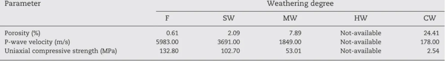
Table 2– Data collected from the literature for checking[16].

Parameter Weathering degree

F SW MW HW CW

Porosity (%) 0.61 2.09 7.89 Not-available 24.41

P-wave velocity (m/s) 5983.00 3691.00 1849.00 Not-available 178.00

Uniaxial compressive strength (MPa) 132.80 102.70 53.01 Not-available 2.54

(7)

networks, the weights are commonly called free parameters

[54]. According to Klimasauskas[55]and Messer and Kittler

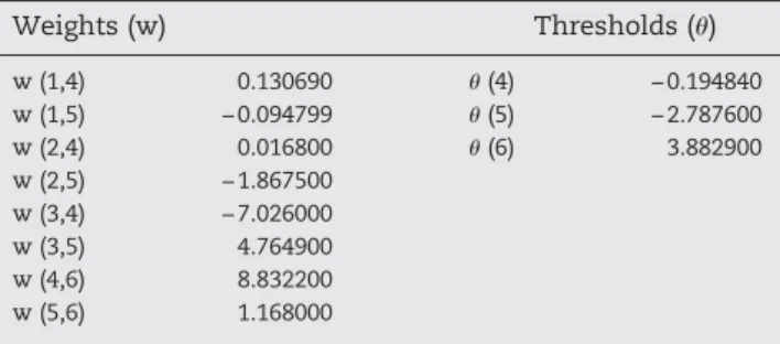
[56], at least 5 to 10 times the number of free parameters should be considered as the required number of training samples. Using the network structure“3-2-1”, the suggestion, proposed by[55,56]is also satisfied more or less for the model developed for the research. Consequently, the constructed artificial neural network models were first trained by the data produced in this study, then compared with the data published by[16]. The sum of square errors (SSE) was used as the convergence criteria during the training stages of the models. For both models the SSE values and the maximum iterations were set to 0.001 and 100, respectively. During the training stages, the SSE value was decreased until approxi-mately 0.006 value for the training data set of the model was reached. This SSE value was obtained in 16 epochs in the model. On the other hand, the SSE value for the check data set was decreased approximately to 0.001. The final network weights and thresholds of the model are shown inFig. 3and

Table 3.

4. Fuzzy Inference System

In this study, the second model for the prediction of weath-ering degree was developed by fuzzy inference system. In classical logic, the membership value of any member is equal to 1 if it is included in the set; if not, that value is equal to 0. These kinds of sets are called“crisp sets”. On the contrary, the members of a fuzzy set can take the membership values ranging between 0 and 1 in fuzzy logic. The term“fuzzy set” was first introduced under the title of“Fuzzy Set Theory” by

[57]. Mathematically, it is commonly defined as follows

(Eq. (2)).

A = fx; μAðxÞgjx∈X ð2Þ

The fuzzy set“A” is represented by a membership function;

μA(x) in the information universe of X. This membership

functionμA(x) defines the membership degree of each member

in the set. Additionally, the degree of membership demonstrates the amount of pertaining level of the member to the fuzzy set. According to Dombi[58], the membership functions require the following properties: (i) all the membership functions should be continuous, (ii) all the membership functions should be described in a certain interval, (iii) the membership functions may be continuously decreasing or increasing, or may have both increasing and decreasing parts together, and (iv) monotonous membership functions may be concave or

convex, or may be concave until a point, and convex here after.

In the literature, there are two different types of fuzzy inference systems that are frequently used. These are the Mamdani and the Takagi–Sugeno–Kang algorithms. The Mamdani algorithm is mostly preferred in engineering geology

[59]. This algorithm was first developed by[60]to be used in a steam machine control. They carried the usage of the steam machine to an upper level and developed a new technique called “if-then” rules. Considering the conventional mathe-matical techniques, integrating this technique to an indirect model seems inapplicable[59]. Alvarez Grima[59]proposed that the Mamdani algorithm constitutes one of the most efficient techniques to solve complex geological engineering problems. The main reason is that the materials studied in engineering geology are commonly natural, and hence they involve a high level of uncertainties. For example, when the weathering description of“high” is used as an input in fuzzy

Table 3– Final model parameters for the constructed artificial neural network architectures.

Weights (w) Thresholds (θ) w (1,4) 0.130690 θ (4) −0.194840 w (1,5) −0.094799 θ (5) −2.787600 w (2,4) 0.016800 θ (6) 3.882900 w (2,5) −1.867500 w (3,4) −7.026000 w (3,5) 4.764900 w (4,6) 8.832200 w (5,6) 1.168000

Fig. 4– Input and output fuzzy sets used in the fuzzy inference system.

(8)

models this term can be expressed by a fuzzy membership function. Due to this flexibility, the fuzzy approach may decrease uncertainties sourced from complexity and hetero-geneity. Based on the Mamdani fuzzy algorithm, several rock mechanics and engineering geology applications have been carried out[61–65].

To reveal properties of any complex and nonlinear system, the“if-then” rules are adapted from the Mamdani algorithm

[66]. The notation of these rules used in the algorithm is commonly given as follows:

R_i: If x_iis A_i1and… and xris Airthen y is Bi i = 1; 2; …; k

where, k is the number of rules, xi (i = 1, 2,…, l) is the input

variable, and y is the output variable. Aijand Bijare the linguistic

terms and Aij(xj) and Bi are the fuzzy sets defined by the

membership functions. The fuzzy sets Aij and Bi should be

defined in the universe of the input and the output spaces. The proposed techniques modified with“if-then” rules have some

linguistic meanings. Such linguistic terms may use “low”,

“moderate”, “high” to indicate the degree of belief. Values of the membership functions should also be defined in the universal linguistic variable space. In the Mamdani fuzzy algorithm, the fuzzy operators such as“and”, “or”, “not” are commonly used to link the input and the output variables. The final output of the Mamdani fuzzy model“B” is also a fuzzy set. However, numerical values are commonly desired in practice. For this reason a defuzzification procedure is required. Defuzzi-fication is briefly defined as the transformation of a fuzzy set into a numerical value. In literature, many defuzzification

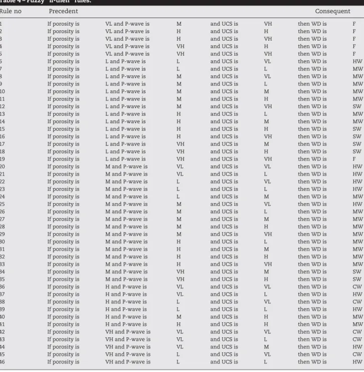
Table 4– Fuzzy “if-then” rules.

Rule no Precedent Consequent

1 If porosity is VL and P-wave is M and UCS is VH then WD is F

2 If porosity is VL and P-wave is H and UCS is H then WD is F

3 If porosity is VL and P-wave is H and UCS is VH then WD is F

4 If porosity is VL and P-wave is VH and UCS is H then WD is F

5 If porosity is VL and P-wave is VH and UCS is VH then WD is F

6 If porosity is L and P-wave is L and UCS is VL then WD is HW

7 If porosity is L and P-wave is L and UCS is L then WD is MW

8 If porosity is L and P-wave is M and UCS is VL then WD is MW

9 If porosity is L and P-wave is M and UCS is L then WD is MW

10 If porosity is L and P-wave is M and UCS is M then WD is MW

11 If porosity is L and P-wave is M and UCS is H then WD is MW

12 If porosity is L and P-wave is M and UCS is VH then WD is SW

13 If porosity is L and P-wave is H and UCS is L then WD is MW

14 If porosity is L and P-wave is H and UCS is M then WD is MW

15 If porosity is L and P-wave is H and UCS is H then WD is SW

16 If porosity is L and P-wave is H and UCS is VH then WD is SW

17 If porosity is L and P-wave is VH and UCS is M then WD is SW

18 If porosity is L and P-wave is VH and UCS is H then WD is SW

19 If porosity is L and P-wave is VH and UCS is VH then WD is F

20 If porosity is M and P-wave is VL and UCS is VL then WD is HW

21 If porosity is M and P-wave is VL and UCS is L then WD is HW

22 If porosity is M and P-wave is L and UCS is VL then WD is HW

23 If porosity is M and P-wave is L and UCS is L then WD is HW

24 If porosity is M and P-wave is L and UCS is M then WD is MW

25 If porosity is M and P-wave is M and UCS is VL then WD is HW

26 If porosity is M and P-wave is M and UCS is L then WD is MW

27 If porosity is M and P-wave is M and UCS is M then WD is MW

28 If porosity is M and P-wave is M and UCS is H then WD is MW

29 If porosity is M and P-wave is M and UCS is VH then WD is MW

30 If porosity is M and P-wave is H and UCS is L then WD is MW

31 If porosity is M and P-wave is H and UCS is M then WD is MW

32 If porosity is M and P-wave is H and UCS is H then WD is MW

33 If porosity is M and P-wave is H and UCS is VH then WD is MW

34 If porosity is M and P-wave is VH and UCS is M then WD is SW

35 If porosity is M and P-wave is VH and UCS is H then WD is SW

36 If porosity is H and P-wave is VL and UCS is VL then WD is CW

37 If porosity is H and P-wave is VL and UCS is L then WD is HW

38 If porosity is H and P-wave is L and UCS is VL then WD is CW

39 If porosity is H and P-wave is L and UCS is L then WD is HW

40 If porosity is H and P-wave is M and UCS is H then WD is MW

41 If porosity is H and P-wave is H and UCS is H then WD is MW

42 If porosity is VH and P-wave is VL and UCS is VL then WD is CW

43 If porosity is VH and P-wave is VL and UCS is L then WD is CW

44 If porosity is VH and P-wave is VL and UCS is M then WD is HW

45 If porosity is VH and P-wave is L and UCS is VL then WD is CW

(9)

methods have been proposed[67]but the center of gravity (COG) method is mostly preferred to be used (Eq. (3)).

y = ∫ SBðyÞydy ∫ SBðyÞdðyÞ ð3Þ In this study, to decrease the uncertainties in the identifica-tion of the weathering degrees of the Harsit granitoid, a Mamdani algorithm was constructed. Porosity, P-wave velocity and uniaxial compressive strength constitute the input vari-ables, which predict the degree of weathering of the rocks. For this purpose, all input and output variables were normalized in advance. Five different fuzzy sets; “fresh”, “slightly

weath-ered”, “moderately weathered”, “highly weathered”, and

“completely weathered” were constructed as the output variables of the degree of weathering. Considering these output fuzzy sets and using the simple regression equations constructed between the input and the output variables before, five different fuzzy sets;“very low”, “low”, “moderate”, “high”, and “very high” were also created for the input variables. Consequently, five for the output variable and 15 for the input variables, a total of 20 fuzzy sets were produced. The fuzzy sets constructed in this study are given below in detail. Addition-ally, graphical representations of these sets are also demon-strated inFig. 4. Fuzzy sets for the input variable“Porosity”

VL = f0=0; 1=0; 1=0:084; 0=0:129g L = f0=0:084; 1=0:129; 0=0:229g M = f0=0:129; 1=0:229; 0=0:41g H = f0=0:229; 1=0:41; 0=0:624g VH = f0=0:41; 1=0:624; 1=1; 0=1g

Fuzzy sets for the input variable“P-wave velocity” VL = f0=0; 1=0; 1=0:2; 1=0:356g

L = f0=0:2; 1=0:356; 0=0:562g M = f0=0:356; 1=0:562; 0=0:769g H = f0=0:562; 1=0:769; 0=0:924g VH = f0=0:769; 1=0:924; 1=1; 0=1g Fuzzy sets for the input variable“UCS”

VL = f0=0; 1=0; 1=0:053; 0=0:148g L = f0=0:053; 1=0:148; 0=0:308g M = f0=0:148; 1=0:308; 0=0:532g H = f0=0:308; 1=0:532; 0=0:793g VH = f0=0:532; 1=0:793; 1=1; 0=1g

Fuzzy sets for the output variable“Weathering degree” F = f0=0:2; 1=0:2; 1=0:25; 0=0:4g

SW = f0=0:25; 1=0:4; 0=0:6g MW = f0=0:4; 1=0:6; 0=0:8g HW = f0=0:6; 1=0:8; 0=0:95g CW = f0=0:8; 1=0:95; 1=1; 0=1g

based on various possible combinations of input fuzzy sets, forty-six“if-then” rules were constructed with the data of the Harsit granitoid (what do you mean). These fuzzy rules are

given in Table 4. To determine the resultant membership

functions that belong to the output parameter weathering degree, the fuzzy operator“max” was implemented. Addition-ally, for the defuzzification of these resultant functions, the center of gravity method was used. Finally, the data set published by[16]was employed to check out the constructed models.

5. Comparison of

Prediction Performances

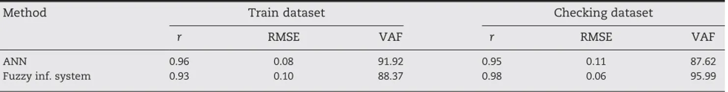
Control performance of a prediction model is an important concern. For this reason, a series of performance analyses was carried out with different performance coefficients such as coefficient of correlation of cross-checks (r), variance account for (VAF) and root mean square error (RMSE). These indices were calculated for training and checking data sets (Table 5). As mentioned earlier, two prediction models were developed employing two soft computing techniques, which are ANN and fuzzy algorithm. The high performance of the training data set shows a good learning capacity of the model while that of checking data set indicates generalization ability of a prediction model. The ANN model performs more effectively while considering three performance indices of the train data set. On the other hand, the fuzzy model performs more effectively while considering the checking data set. This result revealed that the fuzzy model has higher generalization ability than the ANN

Fig. 5– Graph showing the measured and the predicted

weathering degrees of the checking data sets.

Table 5– Prediction performance indices (r, VAF, RMSE) of the models for both training and checking data sets.

Method Train dataset Checking dataset

r RMSE VAF r RMSE VAF

ANN 0.96 0.08 91.92 0.95 0.11 87.62

(10)

model. The checking data set was adapted from a different study[16]. It can be suggested that the prediction models used in the study may be applied for granitic rocks (Fig. 5). However, necessity of the entire dataset of all weathering classes (from 1 to 5) of a granitic rock is the main limitation of the models constructed. It is also suggested that in case of missing input data set, the linguistic fuzzy model should be used under the supervision of an expert. On the other hand, it is impossible to use the ANN model if one or more inputs are missing. In practice, use of both models is easy and can be accepted as reliable, because the models developed in the present study include the test results of all weathering classes of granitic rock. In addition, to apply a normalization procedure contributes to the usability of the models on other granitic rocks. The models developed are data-driven characters. For this reason, if the models are re-constructed by adding new data, some small changes in the membership functions of the fuzzy model and the weights of the ANN model can be expected but a fundamental change may not be encountered. In fact, each data-driven model is open to development. Therefore, the models should be checked by new data despite our claims.

6. Results and Conclusions

The Harsit grainitoid (NE Turkey) was used for this study. Significant changes in porosity, P-wave velocity and uniaxial compressive strength due to the weathering degree, were recorded. Porosity increases with decreasing uniaxial com-pressive strength and P-wave velocity while the degree of weathering increases. Two weathering prediction models with multi-inputs were constructed with two soft computing techniques such as artificial neural networks and fuzzy inference system, considering the difficulties in the determi-nation of weathering classes of the granitic rocks.

The general performances of these techniques are similar. The ANN model performed more effectively than the fuzzy model in learning data set. However, the fuzzy model showed better generalization ability. The performance analyses revealed that the prediction models may be used for granitic rocks, but the character of granitic rock should be similar with the Harsit granitoid. Otherwise, it is possible to obtain erroneous weathering classes.

Necessity of the entire dataset of all weathering classes (from 1 to 5) of a granitic rock is the main limitation of the models constructed. In additional, it should be kept in mind that performance capacities of the models should be com-pared with other data available in literature.

R E F E R E N C E S

[1] Irfan TY. Mineralogy, fabric properties and classification of weathered granites in Hong Kong. Q J Eng Geol 1996;29:5–35. [2] Guan P, Ng CWW, Sun M, Tang W. Weathering indices for

rhyolitic tuff and granite in Hong Kong. Eng Geol 2001;59:147–59.

[3] ISRM R. In: Brown ET, editor. ISRM suggested methods: rock characterization, testing and monitoring. London: Pergamon Press; 1981. p. 211.

[4] Lee S G. Weathering and geotechnical characterization of Korean granites. PhD Thesis, Imperial College, University of London, 1987.

[5] Raj JK. Characterization of weathering profile developed over a porphyritic biotite granite in Peninsula Malaysia. Bull Int Assoc Eng Geol 1985;232:121–30.

[6] Irfan TY, Powell GE. Engineering geological investigations for foundations on a deeply weathered granitic rock in Hong Kong. Bull Int Assoc Eng Geol 1985;32:67–80.

[7] Hencher SR, Martin RP. The description and classification of weathered rocks in Hong Kong for engineering purposes. Proc of the 7th Southeast Asian Geotechnical Conference; 1982. p. 125–42.

[8] ANON. The description and classification of weathered for engineering purposes. Geological Society Engineering Group Working, Party Report. Q J Eng Geol 1995;28:207–42.

[9] Weinert HH. Engineering petrology for roads in South Africa. Eng Geol 1968;2:363–95.

[10] Cole WF, Sandy MJ. A proposed secondary mineral rating for basalt road aggregate durability. Aust Road Res

1980;10(3):27–33.

[11] Onodera TFN, Yoshinaka R, Oda M. Weathering and its relation to mechanical properties of granite. Proc 3rd Cong Int Soc Rock Mech Denver 1974;2A:71–8.

[12] Irfan TY, Dearman WR. The engineering petrography of a weathered granite in Cornwall, England. Q J Eng Geol 1978;11:233–44.

[13] Tugrul A. Weathering effects of engineering properties of Basalt's in Niksar Area.Ph.D. Thesis, Istanbul University, Turkey, 1995 (in Turkish).

[14] Sousa LMO, Suarez del Rio LM, Lope Calleja L, Vicente G, Ruiz e Argandofia VGR, Rey AR. Influence of microfractures and porosity on the physico-mechanical properties and

weathering of ornamental granites. Eng Geol 2005;77:153–68. [15] Goulin R, Yushan L. Engineering geological zonation of

Xiamen granitic weathered crust and bearing capacity of residual soil. 6th International IAEG Congress. Rotterdam: Balkema; 1990. p. 1989–96.

[16] Gupta AS, Rao KS. Weathering indices and their applicability for crystalline rocks. Bull Eng Geol Environ 2001;60:201–21. [17] Kilic R. Geomechanical properties of the ophiolites (Cankiri,

Turkey) and alteration degree of diabase. Bull Int Accoc Eng Geol 1995;51:63–9.

[18] Gokceoglu C, Aksoy H. New approaches for the

characterization of clay-bearing, densely jointed and weak rock masses. Eng Geol 2000;58(1):1–23.

[19] Lan HX, Hu RL, Yue ZQ, Lee CF, Wang SJ. Engineering and geological characteristics of granite weathering profiles in South China. J Asian Earth Sci 2003;21:353–64.

[20] Arikan F, Ulusay R, Aydin N. Characterization of weathering acidic volcanic rocks and a weathering classification based on a rating system. Bull Eng Geol Environ 2007;66:415–30. [21] Ceryan S, Tudes S, Ceryan N. A new quantitative weathering

classification for igneous rocks. Env Geol 2008;55:1319–36. [22] Guven IH. 1/250000 scaled geological and metallogenical map

of the Eastern Black Sea Region: MTA Report 1993 (in Turkish, unpublished).

[23] Boztug D, Debon F, Inan S, Tutkun SZ, Avci N, Kesgin O. Comparative geochemistry of four plutons from the Cretac-eous–Paleogene Central Eastern Anatolian alkaline province. Turk J Eart Sci 1997;6:95–115.

[24] Meulenkamp F, Alvarez Grima M. Application of neural networks for the prediction of the unconfined compressive strength (UCS) from Equotip hardness. Int J Rock Mech Min Sci 1999;36(1):29–39.

[25] Singh VK, Singh D, Singh TN. Prediction of strength properties of some schistose rocks from petrographic properties using artificial neural Networks. Int J Rock Mech Min Sci 2001;38(2):269–84.

(11)

[26] Sonmez H, Gokceoglu C, Nefeslioglu HA, Kayabasi A. Estimation of rock modulus: for intact rocks with an artificial neural network and for rock masses with a new empirical equation. Int J Rock Mech Min Sci 2006;43(2):224–35.

[27] Tunusluoglu MC, Gokceoglu C, Sonmez H, Nefeslioglu HA. An artificial neural network application to produce debris source areas of Barla, Besparmak, and Kapi Mountains (NW Taurids, Turkey). Nat Hazards Earth Syst Sci 2007;7:557–70.

[28] Negnevitsky M. Artificial intelligence: a guide to intelligent systems. England: Addison-Wesley; 2002.

[29] Simpson PK. Artificial neural systems: foundations, paradigms, applications, and implementations. New York: Pergamon Press; 1990.

[30] Maren AJ. A logical topology of neural networks. Proceedings of the second workshop on neural networks, WNN-AIND; 1991. p. 91.

[31] Pham DT. Neural networks in engineering. In: Rzevski G, et al, editor. Applications of artificial intelligence in engineering IX, AIENG/ 94, Proceedings of the 9th International Conference. Southampton: Computational Mechanics Publications; 1994. p. 3–36.

[32] Basheer IA, Hajmeer M. Artificial neural networks: fundamentals, computing, design, and application. J Microbiol Meth 2000;43:3–31.

[33] Looney CG. Advances in feed-forward neural networks: demystifying knowledge acquiring black boxes. IEEE Trans Knowledge Data Eng 1996;8(2):211–26.

[34] Nelson M, Illingworth WT. A practical guide to neural nets. Reading MA: Addison-Wesley; 1990.

[35] Schmidt W, Raudys S, Kraaijveld M, Skurikhina M, Duin R. Initialization, backpropagation and generalization of feed-forward classifiers. Proceeding of the IEEE international conference on neural networks; 1993. 598–604.

[36] Fahlman SE. An empirical study of learning speed in backpropagation. Technical Report CMU-CS-88-162. Carnegie-Mellon University; 1988.

[37] Rumelhart DE, Hinton GE, Williams RJ. Learning internal representation by error propagation. In: Rumelhart DE, McClelland JL, editors. Parallel distributed processing, vol. 1; 1986. p. 318–62.

[38] Watrous RL. Learning algorithms for connectionist networks: applied gradient methods of nonlinear optimisation. Proceedings of the first IEEE Int Conf on Neural Networks, San Diego, vol.2; 1987. p. 619–27.

[39] Jacobs RA. Increased rates of convergence through learning rate adaptation. Neural Netw 1988;1:295–307.

[40] Wythoff BJ. Backpropagation neural networks: a tutorial. Chemometr Intell Lab Syst 1993;18:115–55.

[41] Hassoun MH. Fundamentals of artificial neural networks. Cambridge MA: MIT Press; 1995.

[42] Fu L. Neural networks in computer intelligence. New York: McGraw-Hill; 1995.

[43] Swingler K. Applying neural networks: a practical guide. New York: Academic Press; 1996.

[44] Zupan J, Gasteiger J. Neural networks for chemists: an introduction. New York: VCH; 1993.

[45] Hecht-Nielsen R. Kolmogorov's mapping neural network existence theorem. Proceedings of the first IEEE international conference on neural networks, San Diego CA, USA; 1987. p. 11–4.

[46] Masters T. Practical neural network recipes in C++. Boston MA: Academic Press; 1994.

[47] Hush DR. Classification with neural networks: a

performance analysis. Proceedings of the IEEE international conference on systems Engineering Dayton Ohio, USA; 1989. p. 277–80.

[48] Ripley BD. Statistical aspects of neural networks. In: Barndoff- Neilsen OE, Jensen JL, Kendall WS, editors. Networks and chaos-statistical and probabilistic aspects. London: Chapman & Hall; 1993. p. 40–123.

[49] Paola JD. Neural network classification of multispectral imagery. MSc thesis, The University of Arizona, USA, 1994. [50] Wang C. A theory of generalization in learning machines with

neural application. PhD thesis, The University of Pennsylvania, USA, 1994.

[51] Aldrich C, Reuter MA, Deventer JSJ. The application of neural nets in the metallurgical industry. Miner Eng 1994;7:793–809. [52] Kaastra I, Boyd M. Designing a neural network for forecasting

financial and economic time series. Neurocomputing 1996;10(3):215–36.

[53] Kanellopoulas I, Wilkinson GG. Strategies and best practice for neural network image classification. Int J Remote Sensing 1997;18:711–25.

[54] Yesilnacar E, Topal T. Landslide susceptibility mapping: an comparison of logistic regression and neural networks methods in a medium scale study, Hendek region (Turkey). Eng Geol 2005;79:251–66.

[55] Klimasauskas CC. Applying neural networks. In: Trippi RR, Turban E, editors. Neural networks in finance and investigating. Cambridge: Probus; 1993.

[56] Messer K, Kittler J. Choosing an optimal neural network size to aid search through a large image database. Proceedings of the ninth British machine vision conference (BMVC98), University of Southamton, UK; 1998. p. 235–44. [57] Zadeh LA. Fuzzy sets. Inf Control 1965;8:338–53.

[58] Dombi J. Membership function as an evaluation. Fuzzy Sets Syst 1990;35:1–21.

[59] Alvarez Grima M. Neuro-fuzzy modeling in engineering geology. Rotterdam: A.A. Balkema; 2000. p. 244. [60] Mamdani EH, Assilian S. An experiment in linguistic

synthesis with a fuzzy logic controller. Int J Man-Mach Stud 1975;7:1–13.

[61] Gokceoglu C. A fuzzy triangular chart to predict the uniaxial compressive strength of the Ankara agglomerates from their petrographic composition. Eng Geol 2002;66(1–2):39–51. [62] Sonmez H, Gokceoglu C, Ulusay R. An application of fuzzy sets

to the Geological Strength Index (GSI) system used in rock engineering. Eng Appl Artif Intell 2003;16(3):251–69. [63] Gokceoglu C, Zorlu K. A fuzzy model to predict the uniaxial

compressive strength and modulus of elasticity of a problematic rock. Eng Appl Artif Intell 2004;17:61–72. [64] Nefeslioglu HA, Gokceoglu C, Sonmez H. A Mamdani model to

predict the weighted joint density. Lect Notes Comp Sci (Artif Intell) 2003;2773(I):1052–7.

[65] Nefeslioglu HA, Gokceoglu C, Sonmez H. Indirect

determination of weighted joint density (wJd) by empirical and fuzzy models: Supren (Eskisehir, Turkey) marbles. Eng Geol 2006;85:251–69.

[66] Yager R, Filev DP. Essentials of fuzzy modeling and control. New York: John Wiley and Sons; 1994. 388 pp.

[67] Hellendoorn H, Thomas C. Defuzzification if fuzzy controllers. J Intell Fuzzy Systems 1993;1:109–23.