Ownership, efficiency, and indebtedness: a comparison of private and public firms in Turkey

, . : 9 J

ОwnexsMp/. Efficiency, and în d eb îed n e

S n .r s :

om eanson

Private anb Pablic Firms in Turkey

e ТЬеш s i:emittsd te

D eüartm ent of Е со во іш о

tLe luBíitiite of Scoiioialce

ax.d 3ocm 3Ueace.D of

Umversixy

•*r -p.. . * 'S -?-i. 11»·'f 1 ^ P t " A Г і і і і ш

і'УІПііЛіепі ol tae ReciarstBeiit^

·

J? or ше iJeaTse о*

/г 7-: cıгf^-i“^'p,

я і

>

ф с

тм

t?c*mKímr

O

, E

,

I

:

A COMPARISON

OF

P

P

F

T

A Thesis Submitted to the Department of Economics

and the Institute of Economics and Social Sciences of Bilkent University In Partial Fulfillment of the Requirements for the Degree of

MASTER OF ARTS IN ECONOMICS

by

E>. N«(^¿1/1

B.NiLGUN ERKAYA

t l G

ч г і Ц . з з

• ε / 5

I certify that I have read this thesis and in my opinion it is fully adequate, in scope and in quality, as thesis for the degree of Master of Arts in Economics.

I certify that 1 have read this thesis and in my opinion it is fully adequate, in scope and in quality, as thesis for the degree of Master of Arts in Economics.

Prof Siibi' ogan 1 certify that I have read this thesis and in my opinion it is fully adequate, in scope and in quality, as thesis for the degree of Master of Arts in Economics.

ABSTRACT

OWNERSHIP, EFFICIENCY AND INDEBTEDNESS: A COMPARISON

OF

PRIVATE AND PUBLIC FIRMS IN TURKEY

Nilgun Erkaya M.A. in Economics

Supervisor: Assist. Prof. Izak Atiyas 47 Pages

August, 1997

The public sector in Turkey which was founded in the early 1930’s for the production of basic consumer goods has been accused of being a drain on public resources and of accounting for the bulk of the public deficits since the early 1980’s. This thesis investigates if the effect of efficiency on the distribution of bank credit is different for public and private firms. Firm level efficiencies are estimated from production function and these estimated efficiencies are used to estimate the capital structure equation. The results show that the efficiency of a firm affects its access to bank credit negatively for public sector and positively for private sector.

KEYWORDS: Turkey, Bank Credit, Public Enterprises, Efficiency, Capital Structure

ÖZET

MÜLKİYET, VERİMLİLİK VE BORÇLAR:

TÜRKİYE’DEKİ KAMU VE ÖZEL FİRMALARIN KARŞILAŞTIRILMASI

B. Nilgün Erkaya

Yüksek Lisans Tezi, iktisat Bölümü Tez Yöneticisi: Y. Doç. Dr. İzak Atiyas

47 Sayfa Ağustos, 1997

Türkiye’de ana tüketici mallarını üretmek için 30’lu yıllar başında kurulan kamu sektörü 80’li yıllar başından beridir kamu kaynaklarını kullanmak ve kamu borçlarının sorumlusu olarak görülmektedir. Bu yüksek lisans tezi, verimliliğin banka kredilerinin dağılımı konusunda kamu ve özel sektörlerde farklılık gösterip göstermediğini incelemektedir. Firmalara özel verimlilikler, üretim

fonksiyonlarından tahmin edilip sermaye yapısı eşitliğini tahmin etmek için kullanılmıştır. Sonuçlara göre, kamu firmalarında verimlilik banka kredilerine erişimi ters orantılı bir şekilde etkilerken, özel firmalarda doğru orantılı bir şekilde etkilemektedir.

ANAHTAR KELİMELER: Türkiye, Banka Kredisi, Kamu Teşebbüsler, Verimlilik, Sermaye Yapısı

ACKNOWLEDGEMENTS

1 am grateful to Assist. Prof. Izak Atiyas for his supervision and guidance throughout the development of this thesis. I would like to thank him for his patience and moral support in my hardest days.

I would like to thank also my family who has provided me everything I needed for years. I would like to express my gratitude to them for their financial and moral supports to me in all of my education years. I appreciate the help of my dearest brother, Hakan, who listened to me with patience every time and who is the only person that can make me smile with his jokes from a distance of 580 kilometers.

Special thanks go to my friends Deniz and Hana who always encouraged me and made me survive while preparing this thesis. I would like to express my gratitude to them for listening to all my complaints during thesis preparation period. My last gratitude is to Eray, my one and only physicist, who prevented me from giving up and who was extremely patient with me at the times that I felt exhausted.

Finally, thanks to all these people for not making me feel alone.

CONTENTS PAGE

1 Introduction

2 The Setting

3 Data and Method

3.1 Data

3.1 Econometric Method

4 Indebtedness and EfHciency

4.1 Regressions Using Cross Section Data

4.2 Regressions Using Pooled Data

5 Conclusion Appendix REFERENCES 1 3 1 1 1 1 14 19 22 23 27 28 44

l.INTRODUCTION

In the early 1930’s, the public enterprise sector in Turkey was founded for the aim of producing basic consumer goods. This sector emphasized the production of intermediate goods starting from the early 1960’s. It has a large share in gross capital formation and it has a remarkable impact on aggregate production, employment, and savings. When we consider various forms of government participations, it is true to conclude that more than half of the Turkish economy is owned or controlled by the government. But, since the early 1980’s, the public enterprises have been accused of being a drain on public resources, and accounting for the bulk of the public deficits in Turkey.

The relatively poor performance of the public enterprises has been noticed in both developing and developed countries, and has led most countries to privatize their enterprises. The privatization of public enterprises has encouraged the researchers to compare the performance of public and private enterprises on the basis of efficiency.

On the other hand, the liberalization of the financial markets in Turkey has increased firms’ access to bank credits. Firms are less financially constrained now. There is also evidence that financial resources are allocated more efficiently than before; more specifically, it is found that the correlation between debt and efficiency has become positive after the liberalization took place (Atiyas and Yiilek, 1997).

My aim in this thesis is to compare the allocation of bank credit among public and private firms in Turkey. More specifically, I would like to compare the role of firm-level efficiency in the distribution of credit, controlling other possible determinants of debt. The idea is that while efficiency is expected to have a positive effect on firm-level debt among private firms, this may not be the case among public firms due to the soft budget constraint. Firm level data are used from the annual manufacturing surveys carried out by the State Institute of

Statistics over the period 1985-1993. Firm specific efficiencies are estimated from production functions. The estimates of the efficiencies are then used to estimate capital structure equation for both public and private firms.

I ’he results show that the efficiency of a firm affects its access to bank credit negatively for public sector and positively for private sector. This is an evidence for the difference of public and private firms in their access to bank credit.

The thesis is organized as follows: The next section reviews the public enterprises. The data and the econometric method used to estimate firm level efficiency indices are discussed in chapter 3. Chapter 4 examines estimations of capital structure equation with different regression models and explains the estimation results. Chapter 5 concludes the thesis.

2.THE SETTING

Starting from mid 1930’s, the state assumed the role of the entrepreneurial class and created public enterprises in a broad range of manufacturing activities*. Even after the emergence of the private sector in the late 1940’s, the state still was an agent of industrialization. Electoral politics has supplemented the inertial momentum of public sector expansion^. Even during the 1950’s, when the Demokrat Party pledged itself into privatization, the politicians could not even slow the rate of creation of the SOlZs. In the 1960’s, the military deepened the public enterprise sector in industry to prepare Turkey for entry into the European Common Market (EC), while the politicians of the Adalet Party continued the practices of their Demokrat forerunners. The 1970’s witnessed electorally driven SOE expansion coupled with heavy external borrowing that produced the debt crisis of 1978-1979. This crisis was fueled by the need to finance growing deficits of the state-owned enterprises (SOEs).

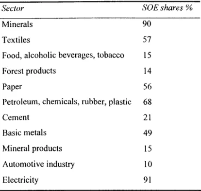
As Turkey entered 1980’s, it had some 32 large holding companies, designated as commercial state economic enterprises (SEEs), and another 10 conglomerates, known as public economic institutions, that were and are official monopolies or provide basic services to the Turkish people. Altogether these holding companies and institutions owned 105 companies and another 40 subsidiaries. In 1985, the industrial SEEs accounted for 45% of the production of the top 500 firms, 27% of total industrial value-added, and 45% of total industrial investment. Table 1 gives sectoral product shares of SOE undertakings:

' See Zaim and Tajkin, 1997. ^ SeeWaterbury, 1993.

TABLE 1. The share o f Turkish SOEs in sectoral production , 1986

Sector SOE shares %

Minerals 90

Textiles 57

Food, alcoholic beverages, tobacco 15

Forest products 14

Paper 56

Petroleum, chemicals, rubber, plastic 68

Cement 21

Basic metals 49

Mineral products 15

Automotive industry 10

Electricity 91

The SOE sector of Turkey has grown to some extent by the acquisition of failing private sector enterprises, or what are called ‘sick’ industries in India. On the other hand, state planners and politicians in Turkey have the common interest of expansion of the SOE sector. The state bankers also share this interest. Specialized lending, especially in the industrial sector, has led over time to the conversion of private debt to public equity.

International donor and commercial creditors for years helped finance SOE expansion in Turkey. After all, the SOE sector constituted a large market the borrowings of which were almost invariably guaranteed by the state treasury. In addition, the SOEs had been obliged to take on unneeded employment and electorally driven wage increases during a period of rapidly rising costs of imported energy. As a result of these, the 1980 stabilization and adjustment program which was market oriented and which had the aim of liberalizing the economy, was not successful in decreasing the reliance of the public enterprises on

the government budget. Hence, SOEs still have a remarkable impact on aggregate production, employment, and savings. The Turkish state maintains a significant if not dominant position in the following list of activities through its SOEs:

power generation railroads

port administration highways

urban transportation telephone and telegraph radio and television media and book publishing construction

agricultural extension irrigation perimeters

textiles iron and steel aluminum, copper petrochemicals fertilizers petroleum products machine tools heavy engineering consumer durables consumer nondurables food and beverages electronics

cars, trucks, buses, tractors

banking and insurance agricultural credit industrial credit small business credit crop purchasing

retail and wholesale trade foreign trade

railroad rolling stock mining (iron, copper,

coal, etc.) defense industries airlines, shipping hotels

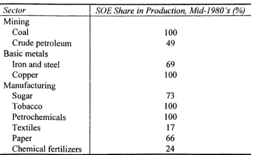
There is no major sector except agricultural production that state has left to private enterprise, and in several sectors the SOEs enjoy a monopolistic or oligopolistic position. Table 2 shows share of SOEs in the production of a certain number of sectors:

TABLE 2. SOE shares in production in Turkey^, mid-1980's (%)

Sector SOE Share in Production, Mid-1980’s (%)

Mining

Coal 100

Crude petroleum 49

Basic metals

Iron and steel 69

Copper 100 Manufacturing Sugar 73 I'obacco 100 Petrochemicals 100 Textiles 17 Paper 66 Chemical fertilizers 24

Expenditures on SOEs in Turkey are much higher than those in industrialized countries'^. The largest items in the expenditures of the industrialized nations are in the area of social services (health, education, and social security), although for some, such as the United States, defense claims a big piece of outlays. Outlays on public enterprise as a proportion of GDP are relatively low, ranging in 1982 between 6% and 11% for a select group including Sweden, France, the United Kingdom, and the United States. But in Turkey, these generalizations do not hold. The ratio of SOE expenditures to GDP is 28% percent in the same years. The level of income does not predict the public sector size. But, what we can conclude is that public enterprise occupies a major place in the overall government expenditures.

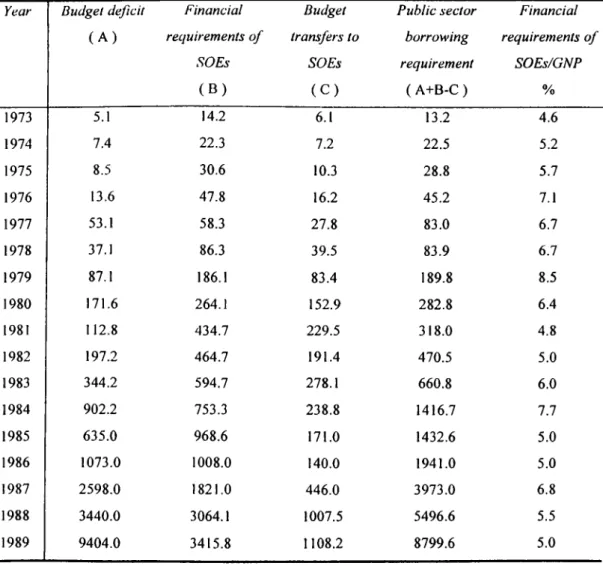
The SOEs have been a drain on public resources, rather than generating surpluses, and they account for the bulk of public deficits in developing countries. The overall deficits of public enterprise sectors are a particularly large component of government deficit in the lesser developed countries (LDCs). For industrial countries overall SOE deficits averaged 2.1% of GDP over the period 1974-1977, while for developing countries the average was 4.6 %. This value for Turkey was 6.1% meaning that Turkey has run much larger deficits than the average for all developing nations. The SOEs constitute a net drain on the treasury and a major contributor to the economic crisis at the end of 1970’s. Table 3 shows this situation:

TABLE 3. Consolidated budget o f Turkey, 1973-89^ (TL billions, current)

Year Budget deficit

( A ) Financial requirements o f SOEs ( B ) Budget transfers to SOEs ( C ) Public sector borrowing requirement ( A+B-C ) Financial requirements o f SOEs/GNP % 1 9 7 3 5.1 1 4 . 2 6 .1 1 3 . 2 4 . 6 1 9 7 4 l A 2 2 . 3 7 . 2 2 2 . 5 5 . 2 1 9 7 5 8 . 5 3 0 . 6 1 0 . 3 2 8 . 8 5 . 7 1 9 7 6 1 3 . 6 4 7 . 8 1 6 . 2 4 5 . 2 7 .1 1 9 7 7 5 3 . 1 5 8 . 3 2 7 . 8 8 3 . 0 6 . 7 1 9 7 8 3 7 . 1 8 6 . 3 3 9 . 5 8 3 . 9 6 . 7 1 9 7 9 8 7 . 1 1 8 6 .1 8 3 . 4 1 8 9 . 8 8 . 5 1 9 8 0 1 7 1 . 6 2 6 4 . 1 1 5 2 . 9 2 8 2 . 8 6 . 4 19 8 1 1 1 2 . 8 4 3 4 . 7 2 2 9 . 5 3 1 8 . 0 4 . 8 1 9 8 2 1 9 7 . 2 4 6 4 . 7 1 9 1 . 4 4 7 0 . 5 5 . 0 1 9 8 3 3 4 4 . 2 5 9 4 . 7 2 7 8 . 1 6 6 0 . 8 6 . 0 1 9 8 4 9 0 2 . 2 7 5 3 . 3 2 3 8 . 8 1 4 1 6 . 7 7 . 7 1 9 8 5 6 3 5 . 0 9 6 8 . 6 1 7 1 . 0 1 4 3 2 . 6 5 . 0 1 9 8 6 1 0 7 3 . 0 1 0 0 8 . 0 1 4 0 . 0 1 9 4 1 . 0 5 . 0 m i 2 5 9 8 . 0 1 8 2 1 . 0 4 4 6 . 0 3 9 7 3 . 0 6 . 8 1 9 8 8 3 4 4 0 . 0 3 0 6 4 . 1 1 0 0 7 . 5 5 4 9 6 . 6 5 . 5 1 9 8 9 9 4 0 4 . 0 3 4 1 5 . 8 1 1 0 8 . 2 8 7 9 9 . 6 5 . 0

One of the reasons for these huge amount of deficits for SOEs lie in the soft budget constraints faced by the public enterprises. In Turkey, financial extravagance is riskless for SOE management, because treasury-guaranteed loans will simply be rolled over (or can be converted into public equity) and until recently enterprises could not legally be liquidated or sold. As long as other sectors of the economy can be taxed (agriculture, mineral exports, worker remittances) and money can be borrowed from abroad, the growing SOE and public deficits can be financed.

In various ways SOEs are indebted to one another. They accumulate substantial arrears in payments for goods and services from other SOEs. The railroads are often victimized by those firms for which they haul goods or move passengers. There can be a kind of imploding chain of missed payments. The railroads may be denied financing for expansion. They delay payment to engineering firms or to iron and steel complexes for goods contracted and delivered. The latter may in turn postpone payment to the electricity authority for power used. Therefore, the more inefficient a public enterprise is, the higher its level of debt is.

The decision to set up a public sector is, therefore, congruent with the decision not to maximize profits. To create a public sector and then ask it to do what the private sector would have done is like going to the cinema to try to sleep rather than see the movie (Amartya Sen, 1975, as cited in Waterbury, 1993).

If credit and product markets are competitive, and if firms are allowed to fail, then public enterprises might be expected to perform as well as private. Sometimes they do. But the conditions mentioned above seldom apply: Credit is subsidized, markets protected, and SOEs prohibited from exit. Because policy makers have structured the competition in this manner, they could also structure it in radically different ways, but they do not.

Whether or not the regulatory regimes are the same, empirical studies tend to show systematic differences in performance between public and private enterprise. The situation is also valid for Turkey. Table 4 shows for Turkey what the impact of an administered increase in SOE prices can do to relative performance indicators. A major increase went through in 1983 with smaller ones in subsequent years. Although the private sector outperformed the public over the seven-year period, by 1985 the SOE profits-sales ratio had surged past the private. In all other areas the private sector maintained a clearly superior position.

TABLE 4 Productivity and rate ofprofit in 500 largest firms in Turkey^ Profit Sales (%) Profit Equity (%) Profit Total assets Value-added Worker ( ‘000 TL) Value added Total assets (%) 1980 1981 1982 1983 1984 1985 1986 Public (79) 4.80 16.16 16.16 2179.T Private (421) 10.47 50.69 50.69 3054.6* Public (64) 3.81 22.04 22.04 3477.8* Private (431) 8.22 42.87 42.87 4831.8* Public (64) 5.49 25.28 25.28 1581.7 23.04 Private (431) 6.47 37.55 37.55 2102.2 39.08 Public (74) 4.44 25.62 25.62 1156.6 14.47 Private (426) 6.88 48.98 48.98 2467.7 35.43 Public (84) 6.45 26.23 26.23 2495.7 20.11 Private (416) 6,99 37.83 37.83 3943.2 33.24 Public (94) 10.77 34.57 34.57 3853.0 17.40 Private (406) 6.05 41.06 41.06 5699.9 33.71 Public (91) 7.80 25.58 25.58 7831.3 27.06 Private (409) 6.09 39.93 39.93 9245.9 35.59

Large deficits in SOEs occur mostly because of the facts that they are politicized and have soft budgets. Electoral pressures cause overemployment and excessively high wages. These favors to the workers return to the new government as huge deficits. However, as the public enterprises have soft budgets, they do not pay their debt. They can postpone it or can get subsidies. Soft budgets enable them to compete without improving efficiency.

By contrast, the private enterprises are more market oriented. Their budget constraints are harder, are less subject to political pressures, and must pay their bills or debts in time. Therefore, they have to compete with improving the efficiency. There is evidence that after liberalization, efficiency of the private firms plays an important role in access to bank credit (Atiyas and Yulek, 1997). They found that the more the efficient the firm is, the more it has access to bank credit.

The correlation between debt and efficiency in private firms is found to be positive in previous research(Atiyas and Yulek, 1997). However, the greater ability of public firms to finance their losses by borrowing from the resources of public (as a result of the soft budget) may result in a negative relation between efficiency and debt levels of the public firms in Turkey.

There are two points to be concerned about the correlation between efficiency and debt levels for public firms due to the fact that the causality can be in two different directions. Firstly, inefficiency can cause easier access to bank credit for public firms. It means that the public firms which are inefficient can finance their debts more easily than the private firms, due to the soft budgets. Secondly, soft budgets, which enable the public firms to accumulate huge deficits, can cause the inefficiency of these firms. This direction of causality implies that the soft budgets faced by public firms, especially in their relation with the public banks, can cause these firms to work inefficiently. Both of these two points may create less positive correlation between debt level and efficiency, or even negative correlation, when we compare the public firms with the private ones. This thesis is really fundamentally concentrating in the first one. The relationship between efficiency and debt level is investigated by estimating capital structure equation both for public and private firms. A comparison of the two kinds of firms in the distribution of credit is done in the end.

Sales from production/number o f workers.

3.DATA AND METHOD

3.1.Data

The empirical research of this thesis is based on information collected by the State Institute of Statistics (SIS) of Turkey. The data set used contain production , cost, investment and a limited set of financial variables for firms that employ more than 10 workers in the manufacturing industry in Turkey. The data is for the period 1985-1993. The data used is a subset of the SIS data set, in the sense that it includes firms that had reported positive values for fixed capital in the 1985 survey. This data set was also used by Atiyas and Ytilek (1997). They also investigated efficiency and debt relationship. I followed their approach in eliminating some of the sectors and used the data set formed by them after eliminations . How they modified the data set can be summarized as follows. Firstly, the sectors that contained less than 150 firms were discarded. Then efficiencies were estimated from the production functions. According to the results of these estimations, two of the remaining sectors which had too noisy efficiency indices were also discarded. There were eight sectors remained after eliminations. The Standard Industrial Classification Codes (SIC) and description of the sectors left after eliminations are as follows: 311-food products, 321- textiles, 322-wearing apparel, 352-other chemicals, 381-metal products, 382-non­ electrical machinery, 383-electrical machinery, 384-transport equipment. The number of firms in the data set per year are presented in Table 1-A. These are the original data set observation numbers before eliminations. How this data set was modified will be discussed below.

The data set includes data on work hours, number of employees, total wage payments, expenditure values such as material, fuel, rent, interest, advertisement, communication, and etc., sales, number and power of electrical and non-electrical machinery, depreciation, internal resources, short-term and long- term bank

See Atiyas and YOlek (1997) for details.

credits, current assets, equity ratios, profits, value added, sum of all long-term financial and physical assets.

In addition, the following data was gathered. First of all, wholesale price indexes (WPI) for each sector were needed. They were collected from the surveys of SIS. Annual WPI, WPI at January prices, and WPI at December prices for each sector for the period 1985-1993 were gathered. These are shown in Table 2-A. These WPI were used to find the real values of value added and sales.

Secondly, the deflators of capital goods were needed. The deflators of machinery, buildings, and fixed capital in average constant 1987 prices and deflator of fixed capital in December in constant 1987 prices were calculated (See Appendix B for details). These deflators are presented in Table 1-B. They were used to calculate the real values of capital goods in average constant 1987 prices. All capital goods except the value of fixed capital were reported in annual average prices. The fixed capital values were reported in December values. So, they were deflated with the calculated December deflator of the corresponding year in constant 1987 prices.

In the production function estimated in the next section, value added is used as the dependent variable. It is the difference between the total output and intermediate goods.

The work hours of each firm was scaled by 10000 and these values were used as indicators of labor input.

The capital input had problems, because physical capital was not reported by the firms. Instead, the financial data included the sum of long term financial and physical assets as well as equity participations in other companies, severance payments, and guarantees. Since that composite variable was not a good measure of the physical capital stock, the physical capital stock series were formed with the

well-known capital law of motion equation which is shown below:

K, = ( \ - 5 ) K , _ , ^ I ,

where K, = capital stock in period t /, = investment in period t

S - depreciation of capital goods

Since the depreciation reported by firms may not represent the economic depreciation of physical assets, 10% was used as the rate of depreciation.

The 85-year capital stock value was taken and the rest of the data was formed by capital law of motion equation. In these calculations, the firms which had any missing data in their investment values and which did not have sequential investment data were eliminated. After eliminating these firms, I formed the physical capital stock series for the rest of the firms in each sector.

This capital data still had distortions in it. Because I started to form the new series with the capital value reported by the firms. The capital stock values became to be closer to the true value when the new estimated values were used, i.e. when the years passed. So, in my estimations I used the interval 1988-1993. In that way, I tried to get rid of most of the distortions in the data. However, that data still was not exactly a good substitute for the true capital value. How I dealt with this problem will be explained in the following section.

In all of my estimations^ I excluded the firms with less than 3 observations in the given period.

Firms had to be classified as public and private. Equity shares of the firms reported in the data set were used for this purpose. Firstly, the observations in which equity shares were misreported were excluded. There were observations of

’ For estimations, LIMDEP is used. It is an econometric software used for estimating the sorts o f regression models most frequently analyzed with cross section data. Its name comes from Limited Dependent Variable Models. 1 used version 6.0 of it.

total equity shares equal to 0% or more than 100%. So, they were excluded before classifying the firms. A firm was classified as “public” if its equity share held by public sector was greater than or equal to 40%, and as “private” otherwise.

3.2.Econometric Method

Firm specific technical efficiencies were estimated using panel data techniques. I began with a Cobb-Douglas representation of technology relating for input and value added in a given industry:

yu - ^ + + A '^ 2ii+ i= 1,...,N

t= 1,...,T

( 1 )

where y is the real value added, x/, ...,x* represent the factors of production, all expressed in logarithms; i is the index representing each firm, t is a time index; a and Pi, ...,Pk are unknown parameters to be estimated, v,, represents random errors.

Ui (iii > 0) represents firm specific technical inefficiency. It is assumed to be

constant for each firm.

The random error Vn is assumed to be iid across firms and time with identical zero mean and constant variance. It is also assumed to be uncorrelated with factor inputs. The other error component, Ui, is assumed to be independently and identically distributed across firms.

Equation (1) can be modified to fit into the standard variable-intercept model for panel data estimations as:

y,, = a, +^iXii( +^2’‘ 2it+...+Pk^kit (2) wh e r e a j =a -Uj

I will use labor input and capital input as factors of production in the estimations. I have no problem with labor input. The true capital is unobservable, and its proxy, the capital stock series I had formed, is not the exact substitute for it. Hence part of disturbance term will reflect capital stock mismeasurement, and the coefficient on capital itself will be biased. So, these measurement error biases have to be corrected. For this aim, instrumental variable estimation'*’ is used. Firstly, I assumed that the ‘true’ capital stock, K*, satisfies the following two equations:

^ ■'■^3X3 + ^ 7 + ( 3 )

K = K ' + 4 ^ (4)

where K = logarithm of the capital stock formed

K* = logarithm of the true capital stock

In this system, Zy, Z?, and Z 3 are the three instruments used for the true

capital stock, ;^and rj are scalar and they are to be estimated by regressions, and

^2 are random disturbances independent of each other with constant means and variances.

Three instrumental variables are used for the true capital stock. The description of them are as follows:

Z, = electricity consumption in kwh

Zj = ^ (Total number of machines - Total number generators) Z3 = ^ (Total power of machines- Total power generators)

Combining equations (3) and (4), the system can be expressed by the observable variables as below:

= y,Z| +^2^2 + ^ 3 ^ 3 + +^2 (5)

See Judge, Griffiths, Llltkepohl and Lee, 1988 for details.

Now the system contain variables which are observed, so I can make estimations of capital stock.

The system of equations needed to estimate firm specific efficiencies are as follows:

and

y,i - +/^2^ii + (6)

where = a

-In order to estimate the efficiencies two stage least square regression model (2SLS) is used. In the first step, I estimated the capital stock values from equation(5) by ordinary least squares approach (OLS). Then I used the fitted values of capital stock estimated from this regression as proxy'' for capital input in equation(6).

Equation(6) is a one factor fixed effects model if a, is treated as fixed and a random effects model if a, is treated as random. The model is shown below:

y,i =OC +

/?,

+

£¡1

where

E[wj = 0, Var[ivJ-£T^, C ov[fj,,uJ = 0

jUi = a + w, where //, is individual specific disturbance

Equation(6) is estimated with both one factor fixed and random effects models and performed Hausman tests to decide which model to use in the rest of the estimations. Hausman test favored the fixed effects model at 0% significance level in each of the 8 sectors. As a result, the efficiencies estimated by fixed effects model is used in the rest of the thesis.

" See Tybout and Corbo, 1991 for details.

The efficiencies estimated by equation(6) are the individual effects excluding the effects of time. 1 then estimated equation(6) by including time effects. The regression model is again fixed effects model but now with 6 time dummies which can be written as follows:

y,,

=

where a , = ¿r -w,

This is a two factor fixed effects model if a, represent a constant for group effects and co, represent a constant lor time effects. It is a two factor random effects model if a, represent a random variable for group effects and a)i represent a random variable for time effects. The variable for time effects is constant across firms. It captures the change in the efficiencies of through years.

A Hausman test was made to decide whether the two factor fixed model or two factor random effects model is better. Hausman test resulted that at 0% significance level two factor fixed effects model is better. So, the results of the two factor fixed effects model was used in the rest of the estimations.

The firm specific efficiencies estimated by one factor and two factor fixed effects models are different from each other. The firm specific efficiencies obtained from one factor model are contaminated by shocks that affect all firms in each year. The firm specific efficiencies estimated from two factor model controls for the possible time effects common to all firms and it purely reflects the firm specific efficiencies. In order to decide which of the models is better, I performed F-tests for each sector. The null hypothesis that the time dummies were all equal to zero was tested. The time effects were significant in all of the sectors. So, I concluded that I will have better estimations for the rest of my models if I use the firm specific efficiencies estimated from the two factor fixed effects model.

The next step is to examine the determinants of indebtedness, and the role of inefficiency in particular, at the firm level. The dependent variable is the ratio

of bank credit to total resources. There were zeros reported for the bank credit variable. Because there was some doubt about which of these were really zero and which were unreported, I used different samples and tried to get rid of observations which were likely to represent misreporting.

Tobit model is used for the models which has censored dependent variable. Censored means that the dependent variable cannot be observed in some range. If it is out of that range, its true value can be observed. If it is in this range, same limit value is observed for all observations, just like observing zero for the bank credit variable in our model.

Besides the Tobit model, other techniques were also used for estimating the leverage equation. The details will be discussed in the next section.

4.INDEBTEDNESS AND EFFICIENCY

In this section, a standard capital structure equation will be estimated. The dependent variable for this equation is the ratio of total bank credits to total resources'^ (BCTR). Firm specific efficiencies are one of the regressors. The section will investigate if the efficiency plays a role in firms’ access to bank credit, and try to find if there are differences in public and private firms in these estimations.

In order to control for the possible misreporting of the bank credit variable by the firms, I formed a restricted sample from which I excluded observations with zero bank credit but positive interest payments. If there were some misreporting in the original sample, then this restricted sample would be less distorted.

The median values of the efficiencies obtained from one factor model (EFFI), the efficiencies obtained from two factor model (EFFT), BCTR, the real value of sales indicating the size of the firms (SIZE), and profitability of the firms (PROFTB) for each sample are given in Table 1-C. The table also presents the number of private and public firms and the number of observations in each sample.

In both the full and the restricted samples, the profitability of private firms are higher than the profitability of the public firms. The median value of profitability (MEDPROFTB ) is negative for public firms and positive for private firms. Taking the restricted sample reduces each of MEDPROFTB.

SIZE indicates that public firms are larger than private firms in both samples. When we take the restricted sample, SIZE becomes smaller in the public sector and becomes larger in the private sector. It means that the observations we

Total resources “ internal resources ^ total bank credit + other debts

excluded as misreported bank credit values are large firms for the public sector and smaller firms for the private sector.

Median value of the ratio of bank debt to total resources (MEDBCTR) for public firms is larger than private firms in both samples. But when we take the restricted sample the difference between them becomes smaller.

The median value of the efficiencies estimated from one factor fixed effects model (MEDEFFI) for public firms are greater than those of the private firms for both of the samples. Again, the difference becomes smaller when restricted sample is used.

The median value of the efficiencies estimated from two factor fixed effects model (MEDEFFT) for public firms are smaller than those of the private firms for both of the samples. The difference becomes larger when the restricted sample is used.

The restricted sample is formed by excluding 16 public firms out of 77 and 125 private firms out of 779. It means that approximately 10% of the firms misreported bank credit variable. The restricted sample can be used to control for the misreport of the firms. On the other hand, the efficiencies estimated by the two factor fixed effects model (EFFT) purely estimates the firm specific efficiencies. As a conclusion, I will use the restricted sample results and EFFT for my comparisons of public and private firms.

There may be several conclusions from the results of Table 1-C. Firstly, although the public firms are larger than private firms, they are less efficient and less profitable than private firms. Secondly, the data suggest that the public firms can get more credits from the banks.

In order to estimate capital structure equation 1 used several regressors that may affect access to bank credit.

F tests performed suggest that EFFT is the variable that should be used to capture firm level efficiency. Below, I used both EFFl and EFFT for the purposes of comparison.

LARGE is used as an indicator of the size of the firm, and is equal to the logarithm of real sales. It is known from literature that larger firms have greater access to bank credit (Bernanke and Gertler, 1995). Smaller firms are more likely to be liquidity constrained in their investment decisions. They are more inclined to take risky projects with the credit they get from the banks. The bank managers know this, so they ration the credit given to the smaller firms more than the large firms. As a result, I will expect positive relationship between LARGE and BCTR.

CFAS is the ratio of cash flow to total assets. It is an indicator of the internal funds of the firm. If the internal funds of the firm is higher, then the firm will need external funds less and use its internal funds for investment according to the well known “pecking order” theory of financing'"' ,i.e., capital structure is driven by firms’ desire to finance new investments, first internally, then with low- risk debt, and finally with equity only as a last resort. According to another point of view, if cash flow of the firm is higher, then it means that tlie firm has higher liquidation value. It is then concluded'^ that debt level increases with the liquidation value of the firm. As a result, 1 will expect negative relationship between CFAS and BCTR.

ADVSA is the ratio of advertisement expenditures to total sales. Advertisement expenditures represent the intangible part of the assets. So, if the advertisement expenditures increase, the liquidation value of the firm decreases. So, 1 expect that ADVSA will be negatively related to BCTR.

MAINCIT is a dummy variable indicating the location of the firm which has value one for large cities (Izmir, Ankara, Istanbul, Adana, Kocaeli, and Bursa). 1 will try to find whether the firms in large cities have greater access to bank credit

See Harris and Raviv 1991. See Harris and Raviv, 1990.

or not. It may be possible that firms in large cities have greater access to bank credit.

Estimations will be carried out for both the full sample and the restricted sample, to see if possible misreporting affects any of the results.

4.1.Regressions Using Cross Section Data

In these estimations, the average value of BCTR was regressed on average values of efficiencies, LARGE, CFAS, ADVSA, and MAINCIT.

Firstly, the capital structure equation was estimated by cross section Tobit regressions and used EFFI as firm specific efficiency (See Table 4-C Panel A for estimation results). For both of the samples, the coefficient of the public sector efficiency is negative and insignificant. This means that whether we take the restricted sample or the full sample, the efficiency of the public firms is not important while they are taking credits from the banks. The coefficient of the efficiency of the private firms is positive and highly significant for both of the samples. The coefficient and the degree of significance increases if we use the restricted sample. This means that the efficiency of the private firms is significantly positively correlated with BCTR. The more efficient firms have more access to bank credit which is consistent with the literature. LARGE is both highly significant and positively correlated with BCTR for both of the samples and for both the public and private firms. It means that the larger the fimi is, the greater is its access to bank credit independent of its being private or public. The coefficient of LARGE for public firms is greater than the coefficient for private firms. The importance of being large for public firms is more than the importance of being large for private firms. CFAS has negative sign but is insignificant for public firms for both of the samples. It is highly significant and has negative sign for private firms for both of the samples. These mean that cash flow of public firms does not have any effect on the access to credit of the public Finns. However, cash

flow, i.e., the internal funds is an important determinant of debt among private firms. Since the cash flow variable captures the costs of external financing associated with agency problems between borrowers and lenders, this result may also suggest that those specific types of agency problems do not characterize the relation between public banks and public firms. It is surprising that ADVSA has positive, very large and highly significant coefficient for public firms and has insignificant coefficient for private firms.. MAINCIT is insignificant for both of the types of the firms indicating that the location of the firm play no role in firm’s access to bank credit.

Secondly, the capital structure equation was estimated by cross section Tobit model using EFFT as firm specific efficiency (See Table 4-C Panel B for estimation results). None of the signs of the coefficients of the variables changed when EFFT was used instead of EFFI. The things that had changed are the significance levels and the coefficients. In the first estimation, EFFI is insignificant for public firms and significant for private firms. But in this regression EFFT is negative and significant for public firms, but insignificant for private firms. It means that the more inefficient a public firm is, the more it has bank credit. The efficiency of the private firms has no effect on their access to bank credit. The significance of LARGE, CFAS, ADVSA, and MAINCIT did not change when EFFT was used as firm specific efficiency.

4.2.Regressions Using Pooled Data

In these estimations, BCTR was regressed on efficiencies, LARGE, CFAS, ADVSA, and MAINCIT. I used the pooled data in these estimations. First kind of the regression used was the Tobit regression. The second is panel data regression models. I tried to find firm specific efficiencies by fixed effects regression. The fixed effects of the capital structure equation are highly correlated with the

efficiencies estimated from the production function. So, I could not use the fixed effects model. Instead of this model, I used random effects model.

Firstly, the capital structure equation was estimated by pooled Tobit regressions and EFFI was used as firm specific efficiency (See Table 5-C Panel A for estimation results). The signs of coefficients and significance of EFFI, LARGE, ADVSA, and MAINCIT are the same as the results of the cross section Tobit estimations done with EFFI. This time CFAS is highly significant and has negative coefficient for both public and private firms and for both of the samples. It means that the more internal funds the firm is, the less it uses bank credit.

Secondly, the capital structure equation was estimated by pooled Tobit regressions and EFFT was used as firm specific efficiency (See Table 5-C Panel B for estimation results). The signs of coefficients and significance of EFFI, LARGE, and ADVSA are the same as the results of the cross section Tobit estimations done with EFFT. CFAS is highly significant and has negative sign for public and private firms in the full sample and for the private firms in the restricted .sample, but it is insignificant for public firms in the restricted sample. MAINCIT is only significant for public sector in the restricted sample with negative sign. It means that if the firm is located in a large city, it has less access to bank credit which conflicts to what I expected.

Thirdly, the capital structure equation was estimated by pooled OLS random effects regressions and EFFI was used as firm specific efficiency (See Table 5-C Panel C for estimation results). ADVSA and MAINCIT are both insignificant for all firms in all samples. EFFI is significant for all private firms whereas it is insignificant for all public firms. The significance and coefficient of EFFI for private firms increase if we use the restricted sample. LARGE is significant and has positive coefficient for all firms. CFAS is only significant for the private firms in the restricted sample with a negative sign.

Finally, the capital structure equation by pooled OLS random effects regressions and EFFT was used as firm specific efficiency (See Table 5-C Panel D

for estimation results). ADVSA and MAINCIT are again insignificant for all firms in all samples. EFFT is significant only for public firms in the full sample and it has negative sign. LARGE is significant and has positive sign for all firms. CFAS is only significant for the private firms in the restricted sample and it has negative sign.

As I explained in the previous section, I did tests for using EFFI or EFFT. According to these results, I had to use EFFT, the efficiency estimated from the one factor fixed effects model. Flence I find estimation results that use EFFT more reliable. It was also argued above that the restricted sample is more likely to avoid observations with misreporting. As result, I will use the estimation results with EFFT and restricted sample for my conclusions.

In all regressions LARGE, the variable indicating the size of the firm, is highly significant with positive coefficient for all firms. So, it can be concluded that the size of the firm affects the access to credit of the firm positively whether the firm is public or private. It means that the larger the firm is, the more it is able to get credit from the banks.

CFAS, the variable indicating the internal resources of the firm, is always highly significant and has coefficient negative for private firms, i.e., the more internal funds a private firm has, the less it needs to obtain external funds from the banks. CFAS is insignificant with the correct sign for public firms. I can conclude that the internal funds of the public firms is not important while taking bank credits. Again, this probably suggests that these specific types of agency problems do not have a strong presence in the public sector.

ADVSA, the variable indicating the intangible part of the assets, is always insignificant with the correct sign for the private firms. I expected it to be significant with a negative coefficient. But, according to my results, the advertisement expenditures of the private firms has no effect on private firms’ access to credit. Except the OLS random effects regression, the ADVSA is .surprisingly significant with a positive and huge coefficient for public firms. I

think there is some misreport of the advertisement expenditures by the firms. So, I do not pay much attention to the results of this variable.

MAINCIT, the variable indicating the location of the firm, is only significant at 5% level in pooled Tobit regression for the public firms. In all other regressions, this variable is insignificant. It means that the location of the firm is not an important factor while taking credit from the banks. The firms in all cities, everything else constant, are equally likely to obtain bank credits.

The variable that concerns this thesis most is the efficiency variable. This variable is always significant and has negative coefficient for public firms except for the OLS random effects model. It can be concluded that the more inefficient public firms have more access to bank credit. Surprisingly, efficiency plays no role in access to credit for private firms according to my estimation results. It is insignificant, but has positive sign as expected.

Results show that the relation between debt and efficiency among private firms is different from that among public firms. For future research, several improvements can be made both in the specification and estimation of the model. Two may be especially important: First, it may be important to control for sectoral differences by including sector dummies. Second, corrections for possible heteroskedasticity in the variance of error terms may be introduced.

5.CONCLUSION

The results can be summarized as follows. Firstly, internal funds is negatively correlated with access to bank credit for the private firms whereas it has no effect on credit for public firms.

Secondly, the size of the firm is an important factor while taking credit for both the public and the private firms. Indebtedness of the larger firms is higher.

Finally, 1 found that efficiency and credit is negatively related for public firms. The efficiency of private firms seems to have no impact on credit according to my results. The coefficient of the efficiency is positive for the private firms, but it is insignificant. I ’his suggests that public firms which are more inefficient can increase their debt levels more as they are supported by the government. It is also possible that soft budget constraints cause lower efficiency in public sector firms, though this hypothesis has not been directly tested in this study. However, the results seem to be consistent with this hypothesis as well. According to these findings, I can conclude that the external finance in public and private firms are not similar. In order to make the public firms work efficiently, they must have either hard budgets or must be privatized.

APPENDIX-A

Table 1 -A

Number o f observations per year and industry in tlie original data set. (The 3 digit Standard Industrial Classification (SIC) codes and the names o f the sectors are as follows: 311-Food products, 321-Textiles, 322-Wearing apparel, 352-Other chemicals, 381-Metal products, 382-Non­ electrical machinery, 383-Flectrical machinery, 384-Transport equipment)

311 321 322 352 381 382 383 384 1985 4 7 6 611 2 4 4 153 3 2 6 2 8 6 2 0 2 189 1986 421 5 3 4 2 1 2 132 2 9 5 2 5 2 1 9 0 178 1987 3 8 8 5 0 5 2 0 6 133 2 7 9 2 5 7 172 166 1988 3 7 4 4 7 3 2 1 3 127 2 4 5 2 2 9 171 154 1989 3 6 5 4 4 8 2 0 2 121 2 2 8 2 1 3 107 143 1990 331 4 3 0 190 123 2 2 3 2 0 3 146 136 1991 301 4 0 3 168 113 2 0 3 177 133 136 1992 2 8 0 3 8 8 146 107 182 167 122 128 1993 3 2 7 4 1 5 162 114 201 185 132 136

Table 2-A

‘^Wholesale price indexes (WPI) in the sectors in years 1985-1993. WPl : Average WPI. It is calculated by taking the average o f

12 months’ WPls.

WPIBEG : WPI in January o f the given year. WPIEND : WPI in December o f the given year.

Panel A: Sector 311

YEAR SECTOR WPI WPIBEG WPIEND

85 311 58 53 73 8 6 311 7 6 73 9 2 8 7 311 100 9 2 1 3 6 8 8 311 184 136 2 2 9 8 9 311 3 1 0 2 2 9 381 9 0 311 4 7 0 381 5 6 7 91 3 i T 7 6 3 5 6 7 9 8 7 9 2 311 1323 9 8 7 1 6 8 2 93 311 2 2 1 4 1 6 8 2 2 9 5 2

Source: St:Ve Institute of Statistics (SIS).

Panel B : Sector 321

YEAR SECTOR WPI WP1I3EG WPIEND

85 321 58 44 60 86 321 76 60 75 87 321 100 75 112 88 321 166 112 189 89 321 249 189 305 90 321 382 305 447 91 321 572 447 711 92 321 980 711 1162 93 321 1552 1162 2153 Panel C: Sector 322

YEAR SECTOR WPI WPIBEG WPIEND

85 322 58 43 59 86 322 76 59 73 87 322 100 73 109 88 322 159 109 183 89 322 259 183 290 90 322 437 290 604 91 322 969 604 1228 92 322 1589 1228 1796 93 322 2103 1796 2608 Panel D: Sector 352

YEAR SECTOR WPI WPIBEG WPIEND

85 352 58 50 69 86 352 76 69 85 87 352 100 85 127 88 352 176 127 214 89 352 302 214 377 90 352 438 377 505 91 352 685 505 792 92 352 993 792 1292 93 352 1543 1292 1755 30

Panel E; Sector 381

YEAR SECTOR WPl WPIBEG WPIEND

85 381 58 48 66 86 381 76 66 83 87 381 100 83 123 88 381 165 123 207 89 381 247 207 292 90 381 373 292 418 91 381 554 418 667 92 381 884 667 1143 93 381 1517 1143 1909 Panel F: Sector 382

YEAR SECTOR WPl WPIBEG WPIEND

85 382 58 63 87 86 382 76 87 108 87 382 100 108 161 88 382 209 161 270 89 382 308 270 372 90 382 503 372 599 91 382 821 599 951 92 382 1235 951 1714 93 382 2011 1714 2380 Panel G: Sector 383

YEAR SECTOR WPl WPIBEG WPIEND

85 383 58 47 65 86 383 76 65 82 87 383 100 82 122 88 383 179 122 204 89 383 266 204 305 90 383 390 305 435 91 383 553 435 630 92 383 970 630 1325 93 383 1732 1325 1949

Panel H: Sector 384

YEAR SECTOR WPI WPIBEG WPIEND

85 384 58 50 69 86 384 76 69 86 87 384 100 86 127 88 384 185 127 214 89 384 276 214 315 90 384 398 315 442 91 384 566 442 641 92 384 980 641 1347 93 384 1725 1347 1955 32

APPENDIX B

CALCULATION OF THE DEFLATORS

FOR CAPITAL GOODS

Deflators for capital goods are obtained from the national accounts, by dividing nominal investment expenditures to expenditures expressed in constant terms:

Nominal gross (fixed capital formation - residential buildings)

Real gross (fixed capital formation - residential buildings) X 100 Capital deilator in average 1987 prices

( K D l ' F A V )

Nominal non - residential buildings formation

Real non - residential buildings formation X 100 = Land and construction deflator in average 1987 prices (BUILDDEF)

Nominal other gross capital formation

Real other capital formation X 100 = Fixed equipment, machienery and equipment and transportation deflator in average 1987 prices

(MACDLF)

In order to calculate these values for all years in the sample period two sources are used, since the complete GNP data could not be found in any one source.

The flrst source'^ contains GNP data for years after 1987. It reports the real GNP in constant average 1987 prices. The second source'* was used for the rest of the data. This source reports real GNP in constant 1968 prices, so they are converted to constant average 1987 prices.

All these deflators are in constant 87 average prices, because all the variables except the value of fixed capital are in aimual average prices. The capital stock data had to be converted to annual average prices with deflators in order to be used in the regressions with the other variables.

17 „_{Ekonomik ve Sosyal Göstergeler”, 1997, DPT (March).}

The capital stock values are reported at the end of each year. So, they are in December prices. I know the current year’s and the next year’s capital deflators in annual average prices based on year 1987. The problem is to find the December capital deflator of current year from these two data. I assumed that the capital deflator growth is logarithmic. It means that I have assumed that capital deflator growth is constant. So, the December deflator is calculated by taking the geometric mean of the two annual deflators. The steps followed are as below :

KDEFAV,(l + g)^ =KDEFAV,^I

KDEFAV, x(KDEFAV,(l + g)^) = KDEFAV, xKDEFAV,,, (KDEFAV,(I + g))^ = KDEFAV, x KDEFAV,_{l + l}

ln (K D E F A V ,(l + g)) = ln (K D E F A V ,)+ ln(K D EFA V ,^i) KDEFAV, (I+ g) = (K DEFAV, x KDEFAV, ^ , ) = KDEFDEC

December capital dellalor

where g : the 6-month growth rate for capital deflator which is assumed to be constant

KDEFAV : capital deflator for each year in constant 1987 prices KDEFDEC: capital deflator for December of each year

in constant 1987 prices

IK ..

TABLE 1-B

I he machinery , building deflators and yearly average and December capital dellators'*^ are given at 1987 constant prices for years 1985-1993.

YEAR MACDEF BEILDDEF KDEFAV KDEFDEC

85 56 49 46 58 86 76 64 72 85 87 100 100 100 132 88 169 193 175 213 89 247 291 260 315 90 356 457 381 481 91 558 769 608 775 92 918 1225 988 1229 93 1405 2087 1530 2381

See the te.xt for source.

APPENDIX-C

TABLE 1-C

Description o f the variables used in explaining the median levels o f some variables in the sample

LABEL DESCRIPTION M E D b m MnDlirn M f-DBCfR SlZli Ml-DPROFfB

Median value o f efficiencies which are estimated by OLS fixed effects regression with firm dummy variables

Median value o f efficiencies which are estimated by OLS fixed effects regression with firm and time dummy variables

Median value o f the ratio o f total bank credit to total assets Median value o f the real sales

Median value o f the profitabilities__________________________________________

TABLE 2-C

Median values o f efficiencies, BCTR, real sales, profitability are given below (variable descriptions are in Table 1-C). Full sample is the sample without restrictions on BC'fR and interest expenditures. The restricted sample excludes the observations with zero bank credits but positive interest expenditures. Firms with less than 3 observations are excluded while forming each o f the samples. Each sample contains observations for the time interval 1988-1993.

PANEL A: FULL SAMPLE

PUBLIC PRIVATE MEDEFFI -0.98960 -1.1092 MEDEFFT -0.15908 -0.031636 MEDBCTR 0.15096 0.18212 SIZE 71052 29767 MEDPROFTB -0.022937 0.075875 Number of firms 77 779 Number of observations 328 3580

PANEL B: RESTRICTED SAMPLE

PUBLIC PRIVATE MEDEI'FI -1.0628 -1.1178 MEDEFFT -0.23174 -0.020072 MEDBCTR 0.22933 0.23628 SIZE 67421 32659 MEDPROFTB -0.02687 0.071786 Number of firms 61 654 Number of observations 249 2806 36

TABLE 3-C

Description o f the variables used in estimations.

LABEL DESCRIPTION BCTR EFFI EFFF LARGE CFAS ADVSA MAINCIT

Ratio o f total bank credit to total resources

Efficiencies estimated by OLS fixed effects regression with firm dummy variables Efficiencies estimated by OLS fixed effects regression with firm and time dummy variables

Logarithm o f real value o f sales The ratio o f cash flow to total assets

The ratio o f advertisement expenditures to sales

The dummy variable indicating the location o f the firm________________________

TABLE 4-C

Cross section Tobit regressions o f group means o f BCTR on the group means o f LARGE, CFAS, ADVSA, MAINCIT and efficiencies. Two regressions are made for each sample: one with EFFI and one with EFFT. Observations are for the time interval 1988-1993. (p-values in parentheses).

DEl’ENDEN'l' VARIABLE INDEPENDENT

VARIABLE

BC'l'R

PANEL A: CROSS-SECTIONAL TOBIT REGRESSIONS USING EFFI

F U LL S A M P L E R E S T R IC T E D S A M P L E

PUBLIC PRIVATE PUBLIC PRIVATE

INTERCEPT -0.694* -0.374* -0.933* -0.268* (0.030) (0.000) (0.011) (0.000) |·;I·FI -0.006 0.003* -0.007 0.005* (0.407) (0.031) (0.345) (0.001) LARGE 0.075* 0.056* 0.099* 0.05* (0.008) (0.000) (0.002) (0.000) CEAS -0.022 -0.033* -0.103 -0.123* (0.335) (0.025) (0.137) (0.000) ADVSA 26.675* -0.065 31.010* 0.221 (0.032) (0.718) (0.014) (0.591) MAINCIT -0.063 0.016 -0.055 0.005 (0.324) (0.297) (0.413) (0.775) r2 0.11“ 0.15“ 0.18“ 0.15“ Number o f observations 77 779 61 654

* represents significance o f the variable at 10% significance level. ‘*R^ from ordinary least squares regression.

PANEL B : CROSS-SECTIONAL TOBIT REGRESSIONS USING EFFT

F U L L S A M P L E R E S T R IC T E D S A M P L E

PUBLIC PRIVATE PUBLIC PRIVATE

INTERCEPT -1.261* -0.367* -1.456* -0.259* (0.001) (0.000) (0.001) (0.000) El^rr -0.128* 0.004 -0.114* 0.005 (0.002) (0.631) (0.015) (0.603) LARGE 0.122* 0.054* 0.145* 0.049* (0.000) (0.000) (0.000) (0.000) CPAS -0.016 -0.031* -0.038 -0.115* (0.473) (0.039) (0.596) (0.000) ADVSA 44.107* -0.050 46.480* 0.268 (0.001) (0.783) (0.001) (0.519) MAINCIT -0.054 0.012 -0.060 0.001 (0.362) (0.410) (0.353) (0.946) 0.18“* 0.14*' 0.22** 0.13** Number o f observations 77 779 61 654 39

Pooled Tobit regressions o f BCTR on LARGE, CFAS, ADVSA, MAINCLI' and efficiencies.Two regressions each are made for each sample : one with EFFI and one with EFFT. Observations are in the time interval 1988-1993. (p-values in parentheses).

TABLE 5-C

DEPENDEN’f VARIABLE INDEPENDENT

VARIABLE

B C fR

PANEL A: POOLED 1 OBIT REGRESSIONS USING EFFI

F U L L S A M P L E R E S T R IC T E D S A M P L E

PUBLIC PRIVATE PUBLIC PRIVATE

INTERCEPT -0.918* -0.578* -0.858* -0.359* (0.000) (0.000) (0.000) (0.000) EFFI -0.008 0.004* -0.008 0.005* (0.158) (0.002) (0.143) (0.000) LARGE 0.084* 0.069* 0.095* 0.058* (0.000) (0.000) (0.000) (0.000) CFAS -0.143* -0.035* -0.067* -0.139* (0.000) (0.000) (0.047) (0.000) ADVSA 15.596* 0.012 12.5* 0.109 (0.022) (0.897) (0.041) (0.361) MAINCIT -0.066 0.013 -0.092* 0.001 (0.216) (0.285) (0.065) (0.990) R2 0.04« 0.08« 0.08« 0.09« Number o f observations 345 3580 249 2806 dO