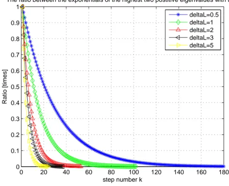
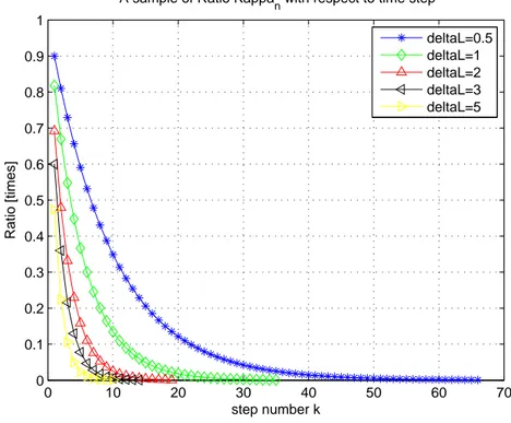
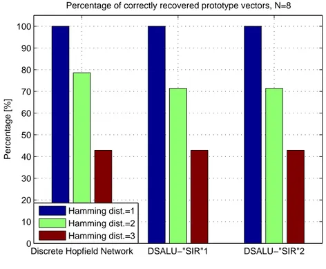
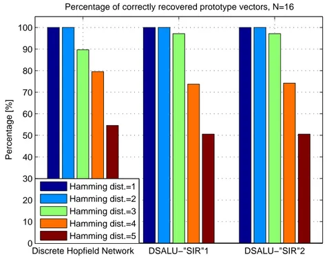
arXiv:0902.3844v1 [physics.data-an] 23 Feb 2009
Analysis of “SIR”
(“Signal”-to-“Interference”-Ratio) in
Discrete-Time Autonomous Linear Networks
with Symmetric Weight Matrices
Zekeriya Uykan
Abstract
It’s well-known that in a traditional discrete-time autonomous linear systems, the eigenvalues of the weigth (system) matrix solely determine the stability of the system. If the spectral radius of the system matrix is larger than 1, then the system is unstable. In this paper, we examine the linear systems with symmetric weight matrix whose spectral radius is larger than 1.
The author introduced a dynamic-system-version of ”Signal-to-Interference Ratio (SIR)” in non-linear networks in [7] and [8] and in continuous-time non-linear networks in [9]. Using the same ”SIR” concept, we, in this paper, analyse the ”SIR” of the states in the following two N -dimensional discrete-time autonomous linear systems: 1) The system x(k + 1) = I + α(−rI + W)x(k) which is obtained by discretizing the autonomous continuous-time linear system in [9] using Euler method; where I is the identity matrix, r is a positive real number, and α >0 is the step size. 2) A more general autonomous linear system descibed by x(k + 1) = −ρI + W x(k), where W is any real symmetric matrix whose diagonal elements are zero, and I denotes the identity matrix and ρ is a positive real number. Our analysis shows that: 1) The ”SIR” of any state converges to a constant value, called ”Ultimate SIR”, in a finite time in the above-mentioned discrete-time linear systems. 2) The ”Ultimate SIR” in the first system above is equal to λρ
max
where λmax is the maximum (positive) eigenvalue of the matrix W. These results are in line with those of [9] where corresponding continuous-time linear system is
Z. Uykan is with Helsinki University of Technology, Control Engineering Laboratory, FI-02015 HUT, Finland, and Nokia Siemens Networks, Espoo, Finland. E-mail: zekeriya.uykan@hut.fi, zuykan@seas.harvard.edu. The author has been a visiting scientist at Harvard University Broadband Comm Lab., Cambridge, 02138 , MA, since September 2008 and this work has been performed during his stay at Harvard University.
examined. 3) The ”Ultimate SIR” in the second system above is equal toλρ
m where λmis the eigenvalue
of W which satisfy |λm− ρ| = max{|λi− ρ|}Ni=1 if ρ is accordingly determined from the interval 0 < ρ < 1.
In the later part of the paper, we use the introduced ”Ultimate SIR” to stabilize the (originally unsta-ble) networks. It’s shown that the proposed Discrete-Time ”Stabilized”-Autonomous-Linear-Networks-with-Ultimate-SIR” exhibit features which are generally attributed to Discrete-Time Hopfield Networks. Taking the sign of the converged states, the proposed networks are applied to binary associative memory design. Computer simulations show the effectiveness of the proposed networks as compared to traditional discrete Hopfield Networks.
Index Terms
Autonomous Discrete-Time Linear Systems, discrete Hopfield Networks, associative memory sys-tems, Signal to Interference Ratio (SIR).
I. INTRODUCTION
Signal-to-Interference Ratio (SIR) is an important entity in commucations engineering which indicates the quality of a link between a transmitter and a receiver in a multi transmitter-receiver environment (see e.g. [4], among many others). For example, let N represent the number of
transmitters and receivers using the same channel. Then the received SIR at receiver i is given
by (see e.g. [4])
SIRi(k) = γi(k) =
giipi(k)
νi+PNj=1,j6=igijpj(k)
, i = 1, . . . , N (1) where pi(k) is the transmission power of transmitter i at time step k, gij is the link gain
from transmitter j to receiver i (e.g. in case of wireless communications, gij involves path
loss, shadowing, etc) and νi represents the receiver noise at receiver i. Typically, in wireless
communication systems like cellular radio systems, every transmitter tries to optimize its power
pi(k) such that the received SIR(k) (i.e., γi(k)) in eq.(1) is kept at a target SIR value, γ tgt i . In
an interference dominant scenario, the receiver background noise νi can be ignored and then
γi(k) =
giipi(k)
PN
j=1,j6=igijpj(k)
The author defines the following dynamic-system-version of “Signal-to-Interference-Ratio (SIR)”, denoted by θi(k), by rewriting the eq.(1) with neural network terminology in [7] and
[8]:
θi(k) =
aiixi(k)
νi+PNj=1,j6=iwijxj(k)
, i = 1, . . . , N (3) whereθi(k) is the defined ficticious “SIR” at time step k, xi(k) is the state of the i’th neuron,
aii is the feedback coefficient from its state to its input layer, wij is the weight from the output
of the j’th neuron to the input of the j’th neuron. For the sake of brevity, in this paper, we
assume the ”interference dominant” case, i.e. νi is negligible.
A traditional discrete-time autonomous linear network is given by
x(k + 1) = Mx(k), x(k) ∈ RN ×1, M ∈ RN ×N, (4)
where x(k) shows the state vector at time t and square matrix M is called system matrix or
weight matrix.
It’s well-known that in the system of eq.(4), the eigenvalues of the weight (system) matrix solely determine the stability of system. If the spectral radius of the matrix is larger than 1, then the system is unstable. In this paper, we examine the linear systems with system matrices whose spectral radius is larger than 1.
Using the same ”SIR” concept in eq.(3), we, in this paper, analyse the ”SIR” of the states in the following two discrete-time autonomous linear systems:
1) The following linear system which is obtained by discretizing the continuous-time linear system ˙x =− rI + Wx in [9] using Euler method:
x(k + 1) = I+ α(−rI + W)x(k) (5) where I denotes the identity matrix,(−rI + W) is the real symmetric system matrix with
zero-diagonal W, and α is the step size.
2) A more general autonomous linear system descibed by
where W is any real symmetric matrix whose diagonal elements are zero, and I denotes the identity matrix and r is a positive real number.
Our analysis shows that: 1) The “SIR” of any state converges to a constant value, called “Ultimate SIR”, in a finite time in the above-mentioned discrete-time linear systems. 2) The “Ultimate SIR” in the first system above is equal to λρ
max where λmax is the maximum (positive) eigenvalue of the matrix W. These results are in line with those of [9] where corresponding continuous-time linear system is examined. 3) The “Ultimate SIR” in the second system above is equal to λρ
m where λm is the eigenvalue of W which satisfy |λm− ρ| = max{|λi− ρ|}
N i=1 if
ρ is accordingly determined from the interval 0 < ρ < 1.
In the later part of the paper, we use the introduced ”Ultimate SIR” to stabilize the (originally unstable) network. It’s shown that the proposed Discrete-Time ”Stabilized”-Autonomous-Linear-Networks-with-Ultimate-SIR” exhibit features which are generally attributed to Discrete-Time Hopfield Networks. Taking the sign of the converged states, the proposed networks are applied to binary associative memory design.
The paper is organized as follows: The ultimate ”SIR” is analysed for the autonomous linear discrete-time systems with symmetric weight matrices in section II. Section III presents the stabilized networks by their Ultimate ”SIR” to be used as a binary associative memory system. Simulation results are presented in section IV, which is followed by the conclusions in Section V.
II. ANALYSIS OF“SIR” INDISCRETE-TIME AUTONOMOUS LINEAR NETWORKS WITH SYMMETRIC WEIGHT MATRICES
In this section, we analyse the “SIR” of the states in the following two discrete-time au-tonomous linear systems: 1) The discrete-time auau-tonomous system which is obtained by dis-cretizing the continuous-time linear system in [9] using Euler method; and 2) A more general autonomous linear system descibed by x(k + 1) = (−ρI + W)x(k), where W is any real
symmetric matrix whose diagonal elements are zero, and I denotes the identity matrix and r is
a positive real number.
A. Discretized Autonomous Linear Systems with symmetric matrix case
˙x = − rI + Wx (7) where ˙x shows the derivative of x with respect to time, i.e., ˙x = dx
dt. In this subsection, we
analyse the following discrete-time autonomous linear system which is obtained by discretizing the continuous-time system of eq.(7) by using well-known Euler method:
x(k + 1) = (I + α(−rI + W))x(k) (8) where I is the identity matrix, r is a positive real number, (−rI + W) is the system matrix, x(k) shows the state vector at step k, and α > 0 is the step size and
rI = r 0 . . . 0 0 r . . . 0 .. . . .. 0 0 0 . . . r N ×N , W= 0 w12 . . . w1N w21 0 . . . w2N .. . . .. ... wN1 wN2 . . . 0 N ×N (9)
In this paper, we examine only the linear systems with symmetrix weight matrices, i.e.,wij =
wji, i, j = 1, 2, . . . , N. It’s well known that desigining the weight matrix W as a symmetric
one yields that all eigenvalues are real (see e.g. [6]), which we assume throughout the paper due to the simplicity and brevity of its analysis.
The reason of the notation in (9) is because we prefer to have the same notation as in [7].
Proposition 1:
In the autonomous discrete-time linear network of eq.(8), let’s assume that the spectral radius of the system matrix (I + α(−rI + W)) is larger than 1. (This assumption is equal to the
assumption that W has positive eigenvalue(s) and r > 0 is chosen such that λmax > r, where
λmax is the maximum (positive) eigenvalue of W). If α is chosen such that 0 < αr < 1, then the
defined ”SIR” θi(k) in eq.(3) for any state i converges to the following constant within a finite
step number for any initial vector x(0) which is not completely perpendicular to the eigenvector
corresponding to the largest eigenvalue of W. 1
1
It’s easy to check in advance if the initial vector x(0) is completely perpendicular to the eigenvector of the maximum
(positive) eigenvalue of W or not. If this is the case, then this can easily be overcome by introducing a small random variable to x(0) so that it’s not completely perpendicular to the mentioned eigenvector.
θi(k ≥ kT) =
r λmax
, i = 1, 2, . . . , N (10) where λmax is the maximum (positive) eigenvalue of the weight matrix W and kT shows a
finite time constant.
Proof:
From eq. (8), it’s obtained
x(k) =I+ α(−rI + W)kx(0) (11) where x(0) shows the initial state vector at step zero. Let us first examine the powers of the
matrix I+ α(−rI + W) in (11) in terms of matrix rI and the eigenvectors of matrix W:
It’s well known that any symmetric real square matrix can be decomposed into
W= N X i=1 λiviviT = N X i=1 λiVi (12)
where {λi}Ni=1 and {vi}Ni=1 show the (real) eigenvalues and the corresponding eigenvectors
and the eigenvectors {vi}Ni=1 are orthonormal (see e.g. [6]), i.e.,
vivj = 1 if i = j, where i, j = 1, 2, . . . , N 0 if i 6= j, (13)
Let’s define the outer-product matrices of the eigenvectors {λi}Ni=1 as Vj = viviT, i =
1, 2, . . . , N, which, from eq.(13), is equal to Vj = I if i = j, where i, j = 1, 2, . . . , N 0 if i 6= j, (14)
where I is the identity matrix. Defining matrix M,
M= I + α(−rI + W) (15) which is obtained as M= (1 − αr)I + N X i=1 βi(1)Vi (16)
where r > 0, α > 0, and where βi(1) is equal to
βi(1) = αλi (17)
The matrix M2 can be written as
M2 = (1 − αr)2I+ N X i=1 βi(2)Vi (18) where βi(2) is equal to βi(2) = α(1 − αr)λi+ (1 − αr + αλi)βi(1) (19)
Similarly, the matrix M3 can be written as
M3 = (1 − αr)3I+ N X i=1 βi(3)Vi (20) where βi(3) is equal to βi(3) = α(1 − αr)2λi+ (1 − αr + αλi)βi(2) (21)
So, M4 can be written as
M4 = (1 − αr)4I+ N X i=1 βi(4)Vi (22) where βi(4) is equal to βi(4) = α(1 − αr)3λi+ (1 − αr + αλi)βi(3) (23)
So, at step k, the matrix (M)k is obtained as
Mk = (1 − αr)kI+ N X i=1 βi(k)Vi (24) where βi(k) is equal to βi(k) = α(1 − αr)k−1λi+ (1 + α(λi− r))βi(k − 1) (25)
Using eq.(17) and (25), the βi(k) is obtained as βi(1) = αλi (26) βi(2) = αλi (1 − αr) + (1 + α(λi− r)) (27) βi(3) = αλi (1 − αr)2+ (1 − αr)(1 + α(λi− r)) + (1 + α(λi− r))2 (28) .. . (29) βi(k) = αλi k X m=1 (1 − αr)k−m(1 + α(λ i− r))m−1 (30) Defining λi = ζi(1 − αr), we obtain (1 − αr)k−m(1 + α(λ i− r))m−1 = (1 − αr)k−1(1 + αζi)m−1 (31)
Writing eq.(31) in eq.(30) gives
βi(k) = αζi(1 − αr)kS(k) (32) where S(k) is S(k) = k X m=1 (1 + αζi)m−1 (33)
Summing −S(k) with (1 + αζi)S(k) yields
S(k) = (1 + αζi)
k− 1
αζi
(34) From eq.(32), (33) and (34), we obtain
βi(k) = (1 − αr)k(1 + αζi)k− (1 − αr)k (35)
Using the definition ζi = λi/(1 − αr) in eq.(35) gives
βi(k) = (1 + α(λi− r)) k
− (1 − αr)k (36)
Mk = (1 − αr)kI+ N X i=1 (1 + α(λi− r)) k Vi− N X i=1 (1 − αr)kV i (37)
Let’s put the N eigenvalues of matrix W into two groups as follows: Let those eigenvalues
which are smaller that r, belong to set T = {λjt}
Nt
jt=1 where Nt is the length of the set; and let those eigenvalues which are larger than r belong to set S = {λjs}
Ns
js=1 where Ns is the length of the set. We write the matrix Mk in eq.(37) using this eigenvalue grouping
Mk = Mtp(k) + Msp(k) (38) where Mtp(k) = (1 − αr)kI− N X i=1 (1 − αr)kV i+ X jt∈T (1 + α(λjt − r)) k Vjt (39) and Msp(k) = X js∈S (1 + α(λjs− r)) k Vjs (40) We call the matrices Mtp(k) and Msp(k) in (39) and (40) as transitory phase part and steady
phase part, respectively, of the matrix Mk.
It’s observed from eq.(39) that the Mtp(k) converges to zero in a finite step number kT because
relatively small step number α > 0 is chosen such that (1 − αr) < 1 and 1 + α(λjt− r) < 1. So,
Mtp(k) ≈ 0, k ≥ kT (41)
Thus, what shapes the steady state behavior of the system in eq.(11) and (15) is merely the
Msp(k) in eq.(40 ). So, the steady phase solution is obtained from eq.(11), (15) and (40) using
the above observations as follows
xsp(k) = Msp(k)x(0) (42) = X js∈S (1 + α(λjs− r)) k Vjsx(0), k ≥ kT (43) Let’s define the interference vector, Jsp(k) as
Jsp(k) = Wxsp(k) (44)
Using eq.(12) in (44) and the orthonormal features in (14) yields
Jsp(k) = X js∈S λjs(1 + α(λjs − r)) k Vjsx(0) (45) First defining Vjx(0) = uj, andξ = 1−αrα , then dividing vector xsp(k) of eq.(43) to Jsp(k) of
eq.(45) elementwise and comparing the outcome with the ”SIR” definition in eq.(3) results in
xsp,i(k) Jsp,i(k) = 1 rθi(k), i = 1, . . . , N (46) = P js∈S(1 + ξλjs) ku js,i P js∈Sλjs(1 + ξλjs)kujs,i (47) In eq.(47), we assume that the uj = Vjx(0) which corresponds to the eigenvector of the largest
positive eigenvalue is different than zero vector. This means that we assume in the analysis here that x(0) is not completely perpendicular to the mentioned eigenvector. This is something easy
to check in advance. If it is the case, then this can easily be overcome by introducing a small random number to x(0) so that it’s not completely perpendicular to the mentioned eigenvector.
From the analysis above, we observe that
1) If all the (positive) eigenvalues greater than r are the same, which is denoted as λb, then
it’s seen from (47) that
θi(k) =
r λb
, i = 1, . . . , N, k ≥ kT (48)
2) Similarly, if there is only one positive eigenvalue which is larger thanr, shown as λb, then
eq.(48) holds.
3) If there are more than two different (positive) eigenvalues and the largest positive eigen-value is single (not multiple), then we see from (46) that the term related to the largest (positive) eigenvalue dominates the sum of the nominator. Same observation is valid for the sum of the denominator. This is because a relatively small increase inλj causes exponential
increase as time step evolves, which is shown in the following: Let’s show the two largest (positive) eigenvalues asλmax andλj respectively and the difference between them as∆λ.
So, λmax = λj+ ∆λ. Let’s define the following ratio between the terms related to the two
highest eigenvalues in the nominator
Kn(k) = (1 + ξλj)k (1 + ξ(λj + ∆λ))k (49) where ξ = α 1 − αr (50)
Similarly, let’s define the ratio between the terms related to the two highest eigenvalues in the denominator as
Kd(k) =
λj(1 + ξλj)k
(λj + ∆λ)(1 + ξ(λj + ∆λ))k
(51) From eq.(49) and (51), since λj
λj+∆ < 1 due to the above assumptions,
Kd(k) < Kn(k) (52)
We plot the ratio Kn(k) in Fig. 1 for some different ∆λ values and for a typical ξ value.
The Figure 1 and eq.(52) implies that the terms related to the λmax dominate the sum of
the nominator and that of the denominator respectively. So, from eq.(47) and (50),
xsp,i(k) Jsp,i(k) = P js∈S(1 + ξλjs) ku js,i P js∈Sλjs(1 + ξλjs) ku js,i → (1 + ξλmax) k λmax(1 + ξλmax)k = 1 λmax , k ≥ kT (53)
4) If the largest positive eigenvalue is a multiple eigenvale, then, similarly, the corresponding terms in the sum of the nominator and that of the demoninator become dominant, which implies from eq.(47), (49) and (51) that xsp,i(k)
Jsp,i(k) converges to
1
λmax as step number increases. Using the observations 1 to 4, eq.(41), the ”SIR” definition in eq.(3), eq.(46) and (47), we conclude that θi(k) = rxsp,i(k) PN j=1,j6=iwijxsp,j(k) = r λmax , k ≥ kT i = 1, . . . , N, (54)
whereλmax is the largest (positive) eigenvalue of the matrix W, and kT shows the finite time
Definition: Ultimate SIR value: In proposition 1, we showed that the SIR in (3) for every state
in the autonomous discrete-time linear networks in eq.(8) converges to a constant value as step number goes to infinity. We call this converged constant value as ”ultimate SIR” and denote as
θult.
B. A more general autonomous linear discrete-time systems with symmetric matrix case
In this subsection, we analyse the following discrete-time autonomous linear system
x(k + 1) = (−ρI + W)x(k) (55) where I is the identity matrix, ρ is a positive real number, and (−ρI + W) is the symmetric
system matrix. The real symmetric matrix W is shown in eq.(9).
Proposition 2:
In the the discrete-time linear system of eq.(55), let’s assume that the spectral radius of symmetric matrix W in (9) is larger than 1, i.e., the maximum of the norms of the eigenvalues is larger than 1.
If ρ is chosen such that
1)
0 < ρ < 1, (56) and
2) Define the eigenvalue(s) λm as
|λm− ρ| = max{|λi− ρ|}Ni=1 > 1 (57)
the eigenvalueλm is unique. (In other words, ρ is chosen in such a way that the equation
eq.(57) does not hold for two eigenvalues with opposite signs. It would hold for a multiple eigenvalue as well, i.e., same sign.)
then the defined ”SIR” (θi(k)) in eq.(3) for any state i converges to the following ultimate
SIR as step number k evolves for any initial vector x(0) which is not completely perpendicular
2 to the eigenvector corresponding to the eigenvalue λ
m in (57) of W.
θi(k ≥ kT) =
ρ λm
, i = 1, 2, . . . , N (58) where λm is the eigenvalue of the weight matrix W which satisfy eq.(57) and kT shows a
finite time constant.
Proof:
From eq.(55),
x(k) = (−ρI + W)kx(0) (59)
where x(0) shows the initial state vector at step zero. Let’s examine the powers of (−ρI + W)
in (59) in terms of the eigenvectors of W using eqs.(12)-(14):
(−ρI + W) = −ρI + N X i=1 ηi(1)Vi (60) where ηi(1) is equal to ηi(1) = λi (61)
The matrix (−ρI + W)2 can be written as
(−ρI + W)2 = ρ2I+ N X i=1 ηi(2)Vi (62) where ηi(2) is equal to ηi(2) = −ρλi+ (λi− ρ)ηi(1) (63)
Similarly, the matrix (−ρI + W)3 can be written as
2
It’s easy to check in advance if the initial vector x(0) is completely perpendicular to the eigenvector of the eigenvalue λm in (57) of W or not. If this is the case, then this can easily be overcome by introducing a small random number to x(0) so
(−ρI + W)3 = −ρ3I+ N X i=1 ηi(3)Vi (64) where ηi(3) is equal to ηi(3) = ρ2λi+ (λi− ρ)ηi(2) (65)
So, at step k, the matrix (−ρI + W)k is obtained as
(−ρI + W)k = (−ρ)kI+ N X i=1 ηi(k)Vi (66) where ηi(k) is ηi(k) = (−ρ)k−1λi + (λi− ρ)ηi(k − 1) (67) So, from (61)-(67) ηi(1) = λi (68) ηi(2) = λi − ρ + (λi− ρ) (69) ηi(3) = λi ρ2− ρ(λi− ρ) + (λi− ρ)2 (70) .. . (71) ηi(k) = λi k X m=1 (−1)k−mρk−m(λ i− ρ)m−1 (72) Defining λi = µiρ, we obtain ρk−m(λi− ρ)m−1 = ρk−1(µi− 1)m−1 (73)
Writing eq.(73) in eq.(72) gives
ηi(k) = λiρk−1S(k) (74) where S(k) is S(k) = k X m=1 (−1)k−1(µi− 1)m−1 (75)
Summing S(k) with (µi− 1)S(k) yields S(k) = (−1) k−1+ (µ i− 1)k µi (76) From eq.(74), (75) and (76), we obtain
ηi(k) = λiρk−1
(−1)k−1+ (µ i− 1)k
µi
(77) Using the definition µi = λi/ρ in eq.(77) gives
ηi(k) = (−1)k−1ρk+ (λi− ρ)k (78)
From eq.(66) and eq.(78),
(−ρI + W)k= (−ρ)kI+ N X i=1 (−1)k−1ρkV i+ (λi− ρ)kVi (79)
Let’s put the N eigenvalues of matrix W into two groups as follows: Let those eigenvalues
which satisfy |λj− ρ| < 1 belong to set T = {λjt}
Nt
jt=1 whereNt is the length of the set; and let all other eigenvalues (i.e. those which satisfy |λj− ρ| > 1) belong to set S = {λjs}
Ns
js=1 where
Ns is the length of the set. Here, ρ is chosen such that no eigenvalue satisfy |λj − ρ| = 1. We
write the matrix (−ρI + W)k in eq.(79) using this eigenvalue grouping as follows
(−ρI + W)k= N tp(k) + Nsp(k) (80) where Ntp(k) = (−ρ)kI+ N X i=1 (−1)k−1ρkV i+ X jt∈T (λjt− ρ) kV jt (81) and Nsp(k) = X js∈S (λjs − ρ) k Vjs (82)
In (81),|λjt−ρ| < 1 from the grouping mentioned above and ρ is chosen such that 0 < ρ < 1, which means that the Ntp(k) converges to zero in a finite step number kT, i.e.,
Ntp(k) ≈ 0, k ≥ kT (83)
Thus, what shapes the steady state behavior of the system in eq.(59) is merely the Nsp(k) in
eq.(82 ). We call the matrices Ntp(k) and Nsp(k) in (81) and (82) as transitory phase part and
steady phase part, respectively, of the matrix Nk.
So, the steady phase solution is obtained from eq.(59), (80) (81) and (82) as follows
xsp(k) = Nsp(k)x(0) (84) = X js∈S (λjs − ρ) kV jsx(0), k ≥ kT (85) Let’s define the interference vector, Jsp(k) as
Jsp(k) = Wxsp(k) (86)
Using eq.(12) in (86) and the orthonormal features in (14) yields
Jsp(k) = X js∈S λjs(λjs− ρ) kV jsx(0) (87)
Defining Vjx(0) = uj, and then dividing vector xsp(k) of eq.(85) to Jsp(k) of eq.(87)
elementwise and comparing the outcome with the “SIR” definition in eq.(3) results in
xsp,i(k) Jsp,i(k) = 1 rθi(k), i = 1, . . . , N (88) = P js∈S(λjs− ρ) ku js,i P js∈Sλjs(λjs − ρ) ku js,i (89) In eq.(89), we assume that the uj = Vjx(0) corresponding to the eigenvector λm in eq.(57)
is different than zero vector. This means that we assume in the analysis here that x(0) is not
completely perpendicular to the mentioned eigenvector. This is something easy to check in advance. If it is the case, then this can easily be overcome by introducing a small random number to x(0) so that it’s not completely perpendicular to the mentioned eigenvector.
Here it’s assumed that the eigenvalue λm satisfying the equation eq.(57) is unique. In other
opposite signs. (It holds for a multiple eigenvalue, i.e., with same sign). Using this assumption (which can easily be met by choosing ρ accoridingly) in eq.(89) yields the following: The term
related to eigenvalue λm in eq.(57) dominates the sum of the nominator. This is because a
relatively small decrease inλj causes exponential decrease as time step evolves, which is shown
in the following: Let’s define the following ratio
κn(k) =
(λjs− ρ)
k
(λjs+ ∆λ − ρ)
k (90)
where ∆λ represents the decrease. Similarly, for denominator κd(k) =
λjs(λjs − ρ)
k
(λjs+ ∆λ)(λjs + ∆λ − ρ)
k (91)
From eq.(90) and (91), since λj
λj+∆ < 1,
κd(k) < κn(k) (92)
We plot some typical examples of the ratio κn(k) in Fig. 2 for some different ∆λ values. The
Figure 2 and eq.(92) implies that the terms related to theλm dominate the sum of the nominator
and that of the denominator respectively. So, from eq.(89)
xsp,i(k) Jsp,i(k) = P js∈S(λjs − ρ) ku js,i P js∈Sλjs(λjs− ρ) ku js,i → (λm− ρ) ku jm,i λm(λm− ρ)kujm,i = 1 λmax , k ≥ kT (93)
where λm is defined by eq.(57). If the largest positive eigenvalue is a multiple eigenvale,
then, similarly, the corresponding terms in the sum of the nominator and that of the demoninator become dominant, which implies from eq.(89), (90)-(93) that xsp,i(k)
Jsp,i(k) converges to
1
λmax as step number evolves.
From eq.(83), and the ”SIR” definition in eq.(3), we conclude from eq.(88)-(93) that
θi(k) = rxsp,i(k) PN j=1,j6=iwijxsp,j(k) = r λm , k ≥ kT i = 1, . . . , N, (94)
where λm is defined by eq.(57), and kT shows the finite time constant (during which the
III. STABILIZED DISCRETE-TIME AUTONOMOUS LINEARNETWORKS WITH ULTIMATE “SIR”
The proposed autonomous networks networks are 1)
x(k + 1) = I+ α(−rI + W)x(k)δ(θ(k) − θult)
(95)
y(k) = sign(x(k)) (96) where W is defined in (9) α is step size, I is identity matrix and r > 0 as in eq.(8), θ(k) = [θ1(k)θ2(k) . . . θN(k)]T, and θult = [θult1 θult2 . . . θultN ]T, and y(k) is the output of the
network. In eq.(95) δ(θ − θult) =
0 if and only if θ(k) = θult,
1 otherwise (97)
We call the network in ref.(95) as Discrete Stabilized Autonomous Linear Networks by Ultimate “SIR”1 (DSAL-U”SIR”1).
2)
x(k + 1) = (−ρI + W)x(k)δ(θ(k) − θult) (98)
y(k) = sign(x(k)) (99) where I is the identity matrix, 1 > ρ > 0 and W is defined in eq.(9), and y(k) is the
output of the network. We call the network in ref.(98) as DSAL-U”SIR”2.
Proposition 3:
The proposed discrete-time networks of DSAL-U”SIR”1 in eq.(95) is stable for any initial vector x(0) which is not completely perpendicular to the eigenvector corresponding to the largest
eigenvalue of W. 3
Proof: The proof of proposition 1 above shows that in the linear networks of eq.(8), the
defined SIR in eq.(3) for state i converges to the constant ultimate SIR value in eq.(10) for any
initial condition x(0) within a finite step number kT. It’s seen that the DSAL-U”SIR”1 in eq.(8)
3
is nothing but the underlying network of the proposed networks SAL-U”SIR”1 without the δ
function. Since the “SIR” in eq.(3) exponentially approaches to the constant Ultimate “SIR” in eq.(10), the delta function eq.(97) will stop the exponential increase once θ(k) = θult, at which
the system outputs reach their steady state responses. So, the DSAL-U”SIR”1 is stable.
Proposition 4:
The proposed discrete-time network DSAL-U”SIR”2 in (98) is stable for any initial vector
x(0) which is not completely perpendicular to the eigenvector corresponding to the eigenvalue
described in eq.(57). 4
Proof: The proof of proposition 2 above shows that in the linear network of (55), the
defined SIR in eq.(3) for statei converges to the constant ultimate SIR value in eq. (58), for any
initial condition x(0) within a finite step number kT. It’s seen that the linear networks of eq.(55)
is nothing but the underlying network of the proposed network DSAL-U”SIR”2 without the δ
function. Since the “SIR” in eq.(3) exponentially approaches to the constant Ultimate “SIR” in eq.(58), the delta function eq.(97) will stop the exponential increase once θ(k) = θult, at which
the system output reach its steady state response. So, the DSAL-U”SIR”2 is stable.
So, from the analysis above for symmetric W and 0 < r < λmax for the SAL-U”SIR”1 in
eq.(95) and 0 < ρ < 1 for the DSAL-U”SIR”2 in eq.(98), we conclude that
1) The DSALU-”SIR”1 and DSALU-”SIR”2 does not show oscilatory behaviour because it’s assured by the design parameter r that ρ, respectively, that there is no eigenvalue on the
unit circle.
2) The transition phase of the ”unstable” linear network is shaped by the initial state vector and the phase space characteristics formed by the eigenvectors of W. The network is stabilized by a switch function once the network has passed the transition phase. The output of the network then is formed taking the sign of the converged states. If the state converges to a plus or minus value is dictated by the phase space of the underlying linear network from the initial state vector at time 0.
4
Choosing the r and ρ in the DSALU-”SIR”1 and DSALU-”SIR”2 respectively such that the
overall system matrix has positive eigenvalues makes the proposed networks exhibit similar features as Hopfield Network does as shown in the simulation results in section IV.
As far as the design of weight matrixrI (ρI) and W is concerned, well-known Hebb-learning
rule ([5]) is one of the commonly used methods (see e.g. [2]). We proposed a method in [7] which is based on the Hebb-learning rule [5]. We summarize the design method here as well for the sake of completeness.
A. Outer products based network design
Let’s assume that L desired prototype vectors, {ds}Ls=1, are given from (−1, +1)N. The
proposed method is based on well-known Hebb-learning [5] as follows:
Step 1: Calculate the sum of outer products of the prototype vectors (Hebb Rule, [5])
Q=
L
X
s=1
dsdTs (100)
Step 2: Determine the diagonal matrix rI and W as follows:
r = qii+ ϑ (101)
where ϑ is a real number and wij = 0 if i = j, qij if i 6= j i, j = 1, . . . , N (102) where qij shows the entries of matrix Q, N is the dimension of the vector x and L is the
number of the prototype vectors (N > L > 0). From eq.(100), qii = L since {ds} is from
(−1, +1)N.
We assume that the desired prototype vectors are orthogonal and we use the following design procedure for matrices A, W and b, which is based on Hebb learning ([5]).
Proposition 5:
For the proposed network DSALU-”SIR”1 in eq.(8) whose weight matrix is designed by the proposed outer-products (Hebbian-learning)-based method above, if the prototype vectors are
orthogonal, then the defined SIR in eq.(3) for any state converges to the following constant ”ultimate SIR” awithin a finite step number
θi(k > kT) =
r
N − L (103)
where N is the dimension of the network and L is the prototype vectors, tT shows a finite
step number for any initial condition x(0) which is not completely orthogonal to any of the raws
of matrix Q in eq.(100). 5
Proof:
The proof is presented in Appendix I.
Corollary 1:
For the proposed DSALU-”SIR”1 to be used as an associate memory system, whose weight matrix is designed by the proposed outer-products (Hebbian-learning)-based method in section III-A for L orthogonal binary vectors of dimension N,
λmax= N − L (104)
where λmax is the maximum (positive) eigenvalue of the weight matrix W.
Proof:
From the proposition 1 and 4 above, the result in proposition 1 is valid for any real symmetric matrix W whose maximum eigenvalue is positive, while the result of proposition 4 is for only the symmetric matrix designed by the method in section III-A. So, comparing the results of the proposition 1 and 4, we conclude that for the network in proposition 4, the maximum (positive) eigenvalue of the weight matrix W is equal to N − L.
5
It’s easy to check in advance if the initial vector x(0) is completely orthogonal to any of the raws of matrix Q in eq.(100) or
not. If so, then this can easily be overcome by introducing a small random number to x(0) so that it’s not completely orthogonal
IV. SIMULATION RESULTS
We take similar examples as in [7], [8] and [9] for the sake of brevity and easy reproduction of the simulation results. We apply the same Hebb-based (outer-products-based) design procedure ([5]) in [7] and [9], which is presented in section III-A. So, the weight matrix W in all the simulated networks (the proposed networks and Discrete-Time Hopfield Network) are the same. In this section, we present two examples, one with 8 neurons and one with 16 neurons. As in [8], traditional Hopfield network is used a reference network. The discrete Hopfield Network [1] is
xk+1 = signWxk (105) where W is the weight matrix and xk is the state at timek, and at most one state is updated.
Example 1:
The desired prototype vectors are
D = 1 1 1 1 −1 −1 −1 −1 1 1 −1 −1 1 1 −1 −1 (106)
The weight matrices rI and W, and the threshold vector b are obtained as follows by using
the outer-products-based design mentioned above and ϑ is chosen as -1 and for the
DSALU-U”SIR”2 network, ρ = 0.5. A= 2I, W= 0 2 0 0 0 0 −2 −2 2 0 0 0 0 0 −2 −2 0 0 0 2 −2 −2 0 0 0 0 2 0 −2 −2 0 0 0 0 −2 −2 0 2 0 0 0 0 −2 −2 2 0 0 0 −2 −2 0 0 0 0 0 2 −2 −2 0 0 0 0 2 0 , ν = 0 (107)
The Figure 3 shows the percentages of correctly recovered desired patterns for all possible initial conditions x(k = 0) ∈ (−1, +1)N, in the proposed DSALU-”SIR”1 and 2 as compared
to traditional Hopfield network.
Letmd show the number of prototype vectors andC(N, K) represents the combination N, K
(such that N ≥ K ≥ 0), which is equal to C(N, K) = N!
(N −K)!K!, where ! shows factorial. In
our simulation, the prototype vectors are from (−1, 1)N as seen above. For initial conditions,
we alter the sign of K states where K=0, 1, 2, 3 and 4, which means the initial condition is
within K-Hamming distance from the corresponding prototype vector. So, the total number of
different possible combinations for the initial conditions for this example is 24, 84 and 168 for 1, 2 and 3-Hamming distance cases respectively, which could be calculated by md× C(8, K),
where md = 3 and K = 1, 2 and 3.
As seen from Figure 3, the performance of the proposed networks DSALU-”SIR”1 and 2 are the same as that of the discrete-time Hopfield Network for 1-Hamming distance case (%100 for
both networks) and are comparable results for 2 and 3-Hamming distance cases respectively.
Example 2:
The desired prototype vectors are
D = 1 1 1 1 1 1 1 1 −1 −1 −1 −1 −1 −1 −1 −1 1 1 1 1 −1 −1 −1 −1 1 1 1 1 −1 −1 −1 −1 1 1 −1 −1 1 1 −1 −1 1 1 −1 −1 1 1 −1 −1 (108)
The weight matrices rI and W and threshold vector b is obtained as follows by using the
outer products based design as explained above. For matrix rI, ϑ is chosen as -2. The other
network paramaters are chosen as in example 1.
W = 0 3 1 1 1 1 −1 −1 1 1 −1 −1 −1 −1 −3 −3 3 0 1 1 1 1 −1 −1 1 1 −1 −1 −1 −1 −3 −3 1 1 0 3 −1 −1 1 1 −1 −1 1 1 −3 −3 −1 −1 1 1 3 0 −1 −1 1 1 −1 −1 1 1 −3 −3 −1 −1 1 1 −1 −1 0 3 1 1 −1 −1 −3 −3 1 1 −1 −1 1 1 −1 −1 3 0 1 1 −1 −1 −3 −3 1 1 −1 −1 −1 −1 1 1 1 1 0 3 −3 −3 −1 −1 −1 −1 1 1 −1 −1 1 1 1 1 3 0 −3 −3 −1 −1 −1 −1 1 1 1 1 −1 −1 −1 −1 −3 −3 0 3 1 1 1 1 −1 −1 1 1 −1 −1 −1 −1 −3 −3 3 0 1 1 1 1 −1 −1 −1 −1 1 1 −3 −3 −1 −1 1 1 0 3 −1 −1 1 1 −1 −1 1 1 −3 −3 −1 −1 1 1 3 0 −1 −1 1 1 −1 −1 −3 −3 1 1 −1 −1 1 1 −1 −1 0 3 1 1 −1 −1 −3 −3 1 1 −1 −1 1 1 −1 −1 3 0 1 1 −3 −3 −1 −1 −1 −1 1 1 −1 −1 1 1 1 1 0 3 −3 −3 −1 −1 −1 −1 1 1 −1 −1 1 1 1 1 3 0 , ν = 0 (109)
The Figure 4 shows the percentages of correctly recovered desired patterns for all possible initial conditions x(k = 0) ∈ (−1, +1)16, in the proposed DSALU”SIR”1 and 2 as compared to
the traditional Hopfield network.
The total number of different possible combinations for the initial conditions for this example is 64, 480 and 2240 and 7280 for 1, 2, 3 and 4-Hamming distance cases respectively, which could be calculated by md× C(16, K), where md = 4 and K = 1, 2, 3 and 4.
As seen from Figure 4 the performance of the proposed networks DSALU-”SIR”1 and 2 are the same as that of Hopfield Network for 1 and 2-Hamming distance cases (%100 for both
networks), and are comparable for 3,4 and 5-Hamming distance cases respectively.
V. CONCLUSIONS
Using the same “SIR” concept as in [7], and [8], we, in this paper, analyse the “SIR” of the states in the following two N-dimensional discrete-time autonomous linear systems:
1) The system x(k + 1) = (I + α(−rI + W))x(k) which is obtained by discretizing the
autonomous continuous-time linear system in [9] using Euler method; where I is the identity matrix,r is a positive real number, and α > 0 is the step size.
2) A more general autonomous linear system descibed by x(k + 1) = −ρI + W x(k), where W is any real symmetric matrix whose diagonal elements are zero, and I denotes the
identity matrix and ρ is a positive real number.
Our analysis shows that:
1) The “SIR” of any state converges to a constant value, called “Ultimate SIR”, in a finite time in the above-mentioned discrete-time linear systems.
2) The “Ultimate SIR” in the first system above is equal to λρ
max whereλmax is the maximum (positive) eigenvalue of the matrix W. These results are in line with those of [9] where corresponding continuous-time linear system is examined.
3) The “Ultimate SIR” in the second system above is equal to λρ
m whereλm is the eigenvalue of W which satisfy|λm− ρ| = max{|λi− ρ|}Ni=1 if ρ is accordingly determined from the
interval 0 < ρ < 1 as described in (57).
In the later part of the paper, we use the introduced “Ultimate SIR” to stabilize the (originally unstable) networks. It’s shown that the proposed Discrete-Time “Stabilized”-Autonomous-Linear-Networks-with-Ultimate-SIR” exhibit features which are generally attributed to Discrete-Time Hopfield Networks. Taking the sign of the converged states, the proposed networks are applied to binary associative memory design. Computer simulations show the effectiveness of the proposed networks as compared to traditional discrete Hopfield Networks.
As far as design of the design of the weight matrices are concerned, we also present an outer-products (Hebbian-learning)-based method, and show that if the prototype vectors are orthogonal in the proposed DSAL-U”SIR”1 network, then the ultimate SIR θult is equal to r
N −L where N
is the dimension of the network and L is the prototype vectors.
APPENDIX I
Proof of Proposition 5:
x(k) =I+ α(−rI + W)kx(0) (110) Let’s denote the system matrix as
M= I + α(−rI + W) (111) From eq.(100) and (102),
W = Q − LI (112)
where L is the number of orthogonal prototype vector. Using eq.(112) in (111) gives
M=1 − α(r + L)I+ αQ (113) and since ds ∈ (−1, +1)N,
Q2 = NQ (114)
where N is the dimension of the system, i.e., the number of states, and Q is given in (100).
Next, we examine the powers of matrix M) since the solution of the system is x(k) = Mkx(0):
First let’s define b and c as follows
b = 1 − α(r + L) (115)
c = 1 − α(r + L − N) (116) From eq.(113) and (115),
M= bI + σ(1)Q (117) where
The matrix M2 is
M2 = b2I+ σ(2)Q (119) where σ(2) is equal to
σ(2) = α(b + c) (120) Similarly, the matrix M2 is obtained as
M3 = b3I+ σ(3)Q (121) where σ(3) is σ(3) = α(b2+ bc + c2) (122) For k = 4, M4 = b4I+ σ(4)Q (123) where σ(4) is σ(4) = α(b3+ b2c + bc2+ c3) (124) So, when we continue, we observe that the k’th power of the matrix M is obtained as
Mk = bkI+ σ(k)Q (125) where σ(k) is σ(k) = α k X m=1 bk−mcm−1 (126)
whereb = 1−α(r+L) and c = 1−α(r+L−N) as defined in eq.(115) and (116), respectively.
Let’s define the following constant ϕ ϕ = b
c =
1 − α(r + L)
Using (127) in (126) results in σ(k) = αck−1 k X m=1 ϕk−m (128)
Summing −σ(k) with ϕσ(k) yields
σ(k) = ϕ
k− 1
ϕ − 1 αc
k−1 (129)
From eq.(125) and (129), the matrix Mk is written as follows
Mk = bkI+ αck−1ϕk− 1
ϕ − 1 Q (130)
Using the definition of b and c in eq.(115) and (116), respectively, in (130) gives
Mk = Mtp(k) + Msp(k) (131) where Mtp(k) = 1 − α(r + L)kI− 1 αN 1 − α(r + L)kQ (132) and Msp(k) = 1 − α(r + L − N)k αN Q (133)
In above equations, the number of network dimension (N) is much larger than the number
of prototype vector (L), i.e. N >> L. In Hopfield networks, theoretically, L is in the range of
%15 of N (e.g. [3]). So, N > r + L by choosing r accordingly. The learning factor positive α is also typically a relatively small number less than 1. Therefore, 1 − α(r + L) < 1 and
1 − α(r + L − N) > 1. This means that 1) the Mtp(k) in eq.(132) vanishes (aproaches to
zero) within a finite step numberkT; and 2) what shapes the steady state behavior of the system
is merely Msp.
We call the matrices Mtp(k) and Msp(k) in (132) and (133) as transitory phase part and
steady phase part, respectively, of the matrix Mk.
So, the steady phase solution is obtained from eq.(11), (131) and (133)
xsp(k) = Msp(k)x(0) (135)
=
1 − α(r + L − N)k
αN Qx(0), k ≥ kT (136)
Let’s define the interference vector, Jsp(k) as
Jsp(k) = Wxsp(k) (137)
From eq.(112), (114) and (137)
Jsp(k) = (Q − LI)xsp(k) (138)
=
1 − α(r + L − N)k
αN (N − L)Qx(0) (139)
So, dividing vector xsp(k) of eq.(136) to Jsp(k) of eq.(138) elementwise and comparing the
outcome with the ”SIR” definition in eq.(3) results in
θi(k) =
r
N − L, i = 1, . . . , N (140)
which completes the proof.
ACKNOWLEDGMENTS
This work was supported in part by Academy of Finland and Research Foundation (Tukis¨a¨ati¨o) of Helsinki University of Technology, Finland.
REFERENCES
[1] J.J. Hopfield and D.W Tank, Neural computation of decisions in optimization problems Biological Cybernetics, vol. :141-146, 1985.
[2] M.K. Muezzinoglu, M.K. and C. Guzelis, A Boolean Hebb rule for binary associative memory design, IEEE Trans.
Neural Networks, vol. 15, nr. 1:195 - 202, Jan. 2004.
[3] M.K. Muezzinoglu, C. Guzelis and J.M. Zurada, An energy function-based design method for discrete hopfield associative memory with attractive fixed points IEEE Trans. Neural Networks, vol. 16, nr. 2:370-378, March 2005 .
[4] T.S. Rappaport, Wireless Communications: Principles and Practice, Prentice-Hall, New York, 1996. [5] D. O. Hebb , The Organization of Behaviour , John Wiley and Sons, New York, 1949.
[6] O. Bretscher, Linear Algebra with Applications, Prentice Hall, 2005.
[7] Z. Uykan, “From Sigmoid Power Control Algorithm to Hopfield-like Neural Networks: “SIR” (“Signal”-to-“Interference”-Ratio)- Balancing Sigmoid-Based Networks- Part I: Continuous Time”, submitted to IEEE Trans. Neural Networks,
December, 2008.
[8] Z. Uykan, “From Sigmoid Power Control Algorithm to Hopfield-like Neural Networks: “SIR” (“Signal”-to-“Interference”-Ratio)- Balancing Sigmoid-Based Networks- Part II: Discrete Time”, submitted to IEEE Trans. Neural Networks, December, 2008.
[9] Z. Uykan, “ Ultimate “SIR” (“Signal”-to-“Interference”-Ratio) in Continuous-Time Autonomous Linear Networks with Symmetric Weight Matrix, and Its Use to ”Stabilize” the Network as Applied to Binary Associative Memory Systems”,
LIST OF FIGURES
1 The figure shows the ratio Kn in eq.(49) for some different ∆λ values (λ = 5, ξ =
0.11). . . 131 2 The figure shows same examples of ratioκnin eq.(90) for some different∆λ values
(λ = 5). . . 132
3 The figure shows percentage of correctly recovered desired patterns for all possible initial conditions in example 1 for the proposed DSALU-”SIR” and Sign”SIR”NN as compared to traditional Hopfield network with 8 neurons. . . 133 4 The figure shows percentage of correctly recovered desired patterns for all possible
initial conditions in example 2 for the proposed DSALU-”SIR” and Sign”SIR”NN as compared to traditional Hopfield network with 16 neurons. . . 134
0 20 40 60 80 100 120 140 160 180 0 0.1 0.2 0.3 0.4 0.5 0.6 0.7 0.8 0.9 1
The ratio between the exponentials of the highest two postitive eigenvalues with time
step number k Ratio [times] deltaL=0.5 deltaL=1 deltaL=2 deltaL=3 deltaL=5
0 10 20 30 40 50 60 70 0 0.1 0.2 0.3 0.4 0.5 0.6 0.7 0.8 0.9 1
A sample of Ratio Kappan with respect to time step
step number k Ratio [times] deltaL=0.5 deltaL=1 deltaL=2 deltaL=3 deltaL=5
Discrete Hopfield Network DSALU−"SIR"1 DSALU−"SIR"2 0 10 20 30 40 50 60 70 80 90 100
Percentage of correctly recovered prototype vectors, N=8
Percentage [%]
Hamming dist.=1 Hamming dist.=2 Hamming dist.=3
Fig. 3. The figure shows percentage of correctly recovered desired patterns for all possible initial conditions in example 1 for the proposed DSALU-”SIR” and Sign”SIR”NN as compared to traditional Hopfield network with 8 neurons.
Discrete Hopfield Network DSALU−"SIR"1 DSALU−"SIR"2 0 10 20 30 40 50 60 70 80 90 100
Percentage of correctly recovered prototype vectors, N=16
Percentage [%] Hamming dist.=1 Hamming dist.=2 Hamming dist.=3 Hamming dist.=4 Hamming dist.=5
Fig. 4. The figure shows percentage of correctly recovered desired patterns for all possible initial conditions in example 2 for the proposed DSALU-”SIR” and Sign”SIR”NN as compared to traditional Hopfield network with 16 neurons.