Digital dual tone multifrequency receiver

J^L. 'À á

^í::;jj α R .5 C £ ;v £ : T K 5 f O ¿ . 5 ■ е з 5

* 9 9 ¿ ,

DIGITAL DUAL TONE MULTIFREQUENCY

-

RECEIVER

A THESIS

SUBMITTED TO THE, DEPARTMENT OF ELECTRICAL AND ELECTRONICS ENGINEERING

AND THE INSTITUTE OF ENGINEERING AND SCIENCES OF BILKENT UNIVERSITY

IN PARTIAL FULFILLMENT OF THE REQUIREMENTS FOR THE DEGREE OF

MASTER OF SCIENCE

By

Ahm et Suat Ekinci

September 1994

Î C S S K O f 56 3 · S '

ZO

IS

■ ;i L

I certify that I have read this thesis and that in my opinion it is fully adequate, in scope and in quality, as a thesis for the degree of Master of Science.

iProf. İDr. Abdullah Atalar (Superv isor)

I certify that Fliave read this thesis and that in my opinion it is fully adequate, in scope and in quality, as a thesis for the degree of Master of Science.

Assoc. Frof. Dr. M. Ali Tan iCo(Co-supervisor)

I certify that I have read this thesis and that in my opinion it is fully adequate, in scope and in quality, as a thesis for the degree of Master of Science.

Prof. Dr. Murat Aşkar

I certify that I have read this thesis and that in my opinion it is fully adequate, in scope and in quality, as a thesis for the degree of Master of Science.

Asst. Prof. Dr. Orhan Arikan

Approved for the Institute of Engineering and Sciences:

Prof. Dr. Mehmet Bar^iy

Director of Institute of Engineenlig and Sciences

ABSTRACT

D IG IT A L D U A L T O N E M U L T IF R E Q U E N C Y R E C E IV E R

Ahm et Suat Ekinci

M .S . in Electrical and Electronics Engineering

Supervisors: Dr. Abdullah Atalar

and

Dr. M . Ali Tan September 1994

In this thesis, a suitable algorithm for detection o f Dual Tone Multifrequency tones is proposed and implemented as a VLSI chip. The algorithm is based on an approximation of correlation. The input signal is correlated with the hardlimited versions of three sinusoids having 7Ty^3 phase difference. Also, a level detector is added to the algorithm. The algorithm only requires addition and subtraction, but no multiplication; and this reduces the complexity of the circuit. The implementation of the algorithm proposed has been realized as a fully integrated digital DTMF receiver chip using semi-custom layout techniques. The final chip is fabricated in 1-^m CMOS technology, and it has a total area of 24.78 mm^.

Keywords : Dual Tone Multifrequency, correlation receivers, frequency detec­ tion.

ÖZET

S A Y IS A L Ç İF T T O N L U Ç O K F R E K A N S L I SİN Y A L A L IC ISI

Ahm et Suat Ekinci

Elektrik ve Elektronik Mühendisliği Bölümü Yüksek Lisans

Tez Yöneticileri: Dr. Abdullah Atalar

ve

Dr, M . A li Tan Eylül 1994

Bu tezde, çift tonlu çok frekanslı sinyallerin sapteınması için bir algoritma önerilmiş ve çok büyük çapta tümleşik yonga olarak gerçeklenmiştir. Al­ goritma bir korelasyon işlenü yaklaşığına dayanmaktadır. Giriş sinyali ara­ larında ;r/3 faz farkı olan üç sinuzoidal dalganın iki değere nicemlenmesiyle elde edilen işaretlerle ilintilendirilmiştir. Algoritmaya bir de düzey saptayıcısı eklenmiştir. Algoritma toplama ve çıkarma işlemlerinden oluşup, çarpma işlemi içermemektedir; bu da devre karmaşıklığını azaltmaktadır. Önerilen algo­ ritmayla gerçekleştirilen sayısal çift tonlu çok frekanslı alıcı yongası ölçümlü gözeler kullanılarak yapılmıştır. Yonga, l-/im CMOS teknolojisi kullanılarak üretilmiştir, toplam alanı 24.78 mm^ dir.

Anahtar Kelimeler : Çift tonlu çok frekanslı, korelasyon tipi alıcılar, frekans saptama.

ACKNOWLEDGEMENT

I would like to express my deep gratitude to my supervisors Dr. Mehmet Ali Tan and Dr. Abdullah Atalar for their guidance, suggestions, and invaluable encouragement throughout the development of this thesis. I would like to thank to Dr. Murat A§kar and Dr. Orhan Arikan for reading and commenting on the thesis.

And special thanks to all Graduate Students in this department for their continuous support.

I would like to thank to TUBITAK AEAGE for providing all the facilities which have made the completion of this study possible.

TABLE OF CONTENTS

1 INTRODUCTION

1

2 DTMF RECEIVERS

5

2.1 Methods for R e c e iv in g ... 6

2.2 The Method U sed ... 12

2.3 How The System is B u ilt ... 17

2.3.1 Detection C ir c u i t ... 20

2.3.2 Decision C ircu it... 21

2.4 A lg o r ith m ... 22

3 IMPLEMENTATION

25

3.1 Detection C ir c u it ... 25 3.1.1 Correlators 28 3.1.2 R O M ... 28 3.1.3 Level D e te c tio n ... 29 3.1.4 Comparison of three p h a s e s ... 30

3.2 Decision C ircu it... 30

3.2.1 Duration and Interval C ounter... 32

3.2.2 C om p a rison ... 32

3.2.3 System Data ... 36

4 SIMULATION RESULTS AND TESTING THE IMPLE­

MENTATION

39

4.1 Frequency D ep en d en ce...

39

4.2

Phase D e p e n d e n c e ...

43

4.3 Simulation R e s u l t s ...

43

4.4 Testing the D e s i g n ...

44

5 CONCLUSIONS

48

APPENDIX

51

A SOURCE FILES

51

A .l Algorithm Im p le m e n te d ... 51

A

.2

Frequency and Phase Dependence... 57

A .

2.1

C -file ...

57

A .

2.2

M a tla b ... 60

A . 3 Circuit Simulation Files ... 61

A .3.1 Top C i r c u i t ... 61

B

SCHEMATICS

65

B . l Correlator and Level D e te c to r... 65

LIST OF FIGURES

1.1 Switching configurations... 2

2.1 Push buttons and touch tones... 6

2.2 Realization of the filter... 7

2.3 Another realization of the same filter... 8

2.4 Rademacher functions ... 10

2.5 Cl and ... 10

2.6 Functional diagram of the digital multi frequency tone detector in Proudfoot... 11

2.7 Flow chart of the detection algorithm... 13

2.8 Flow chart of the decision algorithm... 14

2.9 The receiver block diagram... 15

2.10 Frequency response for the different algorithms... 15

2.11 Frequency response for the conventional correlation receiver. . . 16

2.12 Frequency response for the algorithm proposed by Proudfoot. 16 2.13 Frequency response for our algorithm... 16

2.14 Output of the first correlator. (Low frequencies) 18

2.15 Output of the corresponding co rr e la to r... ig

2.16 Output of the first correlator. (High frequencies) ... 19

2.17 Output of the corresponding co rr e la to r... 19

2.18 Frequency detection... 20

2.19 Decision Block Diagram... 21

2.20 Phases . . ... 22

2.21 Multiplication and accumulation ... 23

3.1 The correlator block diagram... 29

3.2 two-bit co m p a ra to r... 31

3.3 subblock compcella... 31

3.4 subblock compcellb... 31

3.5 The absolute comparison of three inputs... 32

3.6 Circuit giving the maximum of three inputs... 33

3.7 Comparison with level...34

3.8 Decision circuit s c h e m a t ic ... 35

3.9 The duration counter... 36

3.10 The interval counter... 37

4.1 Frequency dependence of the first three correlators ... 40

4.2 Frequency dependence of the first three correlators ... 41

4.3 Outputs after the absolute m axim u m ... 42

4.4 Outputs after the absolute m axim u m ... 42

4.5 Frequency dependence of the 7’th three correlators ... 43

4.6 Frequency dependence of the seventh three correlators ...44

4.7 Phase dependence of the sixth correlation (labels in degree) . . 45

4.8 top schematic including the multiplexors for test ... 47

B .l The correlator schematic... 65

B.2 Correlation... 66

LIST OF TABLES

2.1 The signaling frequencies in Hz.

2.2 Specifications for multifrequency push-button r e c e iv in g ... 7

3.1 Cells in the hierarchy of the DTMF receiver circuit ₂₆

3.2 Cells in the hierarchy of the DTMF receiver c i r c u i t ... 27

3.3 The multiplier ₃₀

3.4 Conversion Map ₃₈

4.1 Response of the system ₄₆

Chapter 1

INTRODUCTION

Telephony, first invented by Alexander Graham Bell and patented in the USA in 1876, is perhaps the most important means of long-distance communica­ tion. Telephony is the transmission of sound to a distant place. The literal translation of ‘ telephone’ from the Greek means ‘long distance-voice’ [1].

On February 14, 1876 Bell applied for a patent, and on March 7 it was issued. However, first demonstration was not until 10th of March. The first service was a private-line service. Then a number of telephones were connected to the same line, but everyone could hear everyone’s talk, there was no privacy {party-line service). (Shown in Fig. 1.1). Then, the thought of centralized switching arose. Many lines come to a “central office” or “exchange” , and the switching occurs there. Exchange telephone service was invented in 1878 allowing 21 customers to reach each other by means of a central switchboard. Most of the exchanges serve at most 10,000 customers (i.e. 4 digits should be used to represent the numbers). The switchboard was operated manually, the first automated switchboard was invented by Almon B. Strowger in 1892. As the number of telephones grows up, more central offices were created each serving a nearby area and the lines connecting these offices are called trunks. The centralized switching of trunks are performed at a switching office called tandem office. New switching needed to be developed to serve long-distance or toll circuits between cities. Toll offices were thus devised to perform switching of toll trunks only. [2, 3]

In late 1879, telephone numbers were used for the first time. In 1896 A.E. Keith, J. Erickson, and C.J. Erickson, all associates of Strowger, invented a

prívate line

party line

centralized trunking switching

Figure 1.1: Switching configurations.

rotating finger-wheel for dialing the desired telephone number.

In todays telephony systems, “calling customer” dials the number on the telephone handset and the number is relayed to the exchange by one of the following two signalling methods:

• “loop” and “disconnect” pulsing • “multifrequency” tone signalling

“Loop” and “disconnect” pulsing or in other words LD signalling is the older of the two methods. The line is disconnected and re-looped in a very rapid sequence. A pulse of disconnection is obtained. The number of pulses are used to indicate digits of the destination number. One pulse for “ 1” , two pulses for “2” , . . . , ten pulses for “0” . The pulses are repeated at a frequency of 10 per second. So 0 will take a whole second. There is also a gap between two sequences of pulses representing two numbers which is called inter-digit pause (IDP).

Multifrequency signalling, in which the digits are relayed much faster, is a more recent invention, and it has been spreading all around the world. The exchange is alerted by looping the line, but the digits are dialled as a number of short bursts of tones. Rather than detecting the disconnect pulses, the

exchange should detect the frequency of the tones. Multifrequency signalling is also called DTM F signalling where DTMF stands for dual-tone multifrequency. [1, 2, 3].

The problem of tone detection arises here. Many scientists have dealt with detection of DTMF tones problem.

First, analog MF receivers have been used. These have employed a bank of six filters to determine the signalling frequencies. The filters have been followed by detectors producing outputs proportional to power of the frequency components. And finally these outputs and the power of the input signal have been used to determine the correct tones. The likelihood of digit simulation which is the false detection because of the similar tones at the presence of speech hcis been reduced by the timing specifications of digit and pause durations.

It has been then proposed to use digital receivers to reduce the costs [4]. Koval has used DFT in his receiver, and “its performance was as good as conventional analog receiver” .

M. J. Callahan has made a single integrated-circuit receiver[5]. He has proposed two filters to separate the high group and low group components. Then the periods of the signals have been counted to come to a decision. The filters have been located off chip. Then, another DTM F receiver; combining filters, zero crossing detectors and amplitude detectors, has been fabricated [6].

There are also other methods proposed containing digital filters. Instead of analog reception digital reception is used in order to reduce the filter orders, because PCM data is converted from the input signals that are bandlimited to 4kHz [7]. The output of this input filter is then separated by two band- elimination filters. These filters are followed by limiters which drive the band­ pass filters which have been tuned to the correct frequencies. All of these are done by a single DSP chip.

Nonrecursive digital filters can also be used in DTM F receivers [8]. Here two linear phase filters with 7t/2 phase difference should be used to eliminate

the input phase dependence. The outputs of these filters are squared and added. It is seen that linear phase filters are as good as filters without phase constraints.

have been used for determining the presence of a tone. These three moments measure the power, power mean frequency and RMS power bandwidth of the signal. This implementation has required quadrature detection, two lowpass filters and digital differentiation logic to obtain three moments. Detection logic has followed these.

A well-known method of detection of tones with unknown phase in white Gaussian noise is to correlate the input signal with the sine and cosine of the frequency to be detected. To reduce the complexity of the circuit several methods have been proposed. [10, 11, 12]

The algorithm that has been described in [10] is based on the correla­ tion principle where the signals to be correlated are transformed into binary signals that have approximately the same correlation function. Such transfor­ mations have been described in [13]. In this paper, two linear combinations of Rademacher functions have been used as auxiliary signals in correlator. A.D. Proudfoot has explained [12] an algorithm based on a correlation with hardlimited versions of sine and cosine. It is extended in this thesis and used to implement a receiver. In [11] a digital correlator for detecting the multiple signal has been described. The correlation is simplified to a summing accu­ mulator using four multiplications at a time. This introduces more hardware than the previous ones as it includes multiplicators (or ROMs) in it.

A DTM F receiver using synchronous additions and subtractions hcis been proposed in [14], which is a simplification of the correlation into a series of additions and subtractions. It has been done by sampling the input signal at four times each frequency involved. The results have been supported by minimum signal to noise ratio, the ratio of maximum accumulated and sam­ pled values, number of zero crossings and the number of extremes in order to reduce digit simulation and detector has been implemented by using an 8-bit microcomputer without any special hardware.

In the next chapter, the basis for the correlation algorithms are explained with some different approaches. The implementation of the design is described in Chapter 3, and computer simulation results are shown in Chapter 4.

Chapter 2

DTM F RECEIVERS

Technical features of the push-button telephone sets are explained in the recom­ mendations of the CCITT^ In recommended multi frequency code the dialing signal is composed of two frequencies emitted simultaneously when a button is pressed. It is planned to have 10 decimal digits and 6 reserve signals. The two frequencies composing each signal are taken from two mutually exclusive frequency groups of four frequencies each, a code known as the “2 (1/4) code” ^. The low and high group frequencies are shown in Table 2.1. In Fig. 2.1, the

low group high group

697 1209

770 1336

852 1477

941 1633

Table 2.1: The signaling frequencies in Hz.

push button frequencies are shown. There are 10 decimal digits and 6 reserve signals making 16 signals altogether.

Characteristics of multifrequency push-button (MFPB) telephone sets us­ ing voice frequency signals are included in Recommendation Q.23, and Rec­ ommendation Q.24 is for application in local exchanges for the reception of MFPB signals. There are recommendations for various characteristics of such

* Recommendation Q.23 ^Recommendation Q.23

Ffvifici«i:«K (K i) U n . I4>J 6 9 7

□ □ □ □

7 7 0

□ □ □ □

t S 2

□ □ □ □

941

□ □ □ □

Figure 2.1: Push buttons and touch tones.

receivers. Each signal consists of two frequencies taken from mutually exclusive frequency groups of four frequencies each, eis shown in Fig. 2.1 and Table 2.1. The exchange should check for simultaneous presence of one and only one fre­ quency from each group. It should respond to signals having frequencies within the tolerances for MFPB sending (±1.8 % of the frequency). Wider tolerances may be appropriate to tolerate the disturbances during the transmission. The reception characteristics may take the advantage of a limitation, if specified, on maximum difference in power levels of the two frequencies composing the tone. This is also called the twist. The exchange should recognize signals whose duration exceed the minimum expected value from subscribers to guard against false signal indications. Similarly pause intervals greater than a speci­ fied value should be recognized by the exchange. The receiver should operate properly at the presence of speech and a dial tone. These recommendations do not supersede the existing national specifications. In Table 2.2, the val­ ues of multifrequency push-button receiving parameters adopted by various administrations are shown.

The algorithm proposed in this thesis satisfies the specifications (Table 2.2) of frequency tolerance and power level difference between frequencies.

2.1

Methods for Receiving

For detecting a tone the first thing to be done is finding the frequency compo­ nents of the input signal. As there are finite number of tones to be detected the problem reduces to detection of only those frequencies that can form a valid

Parameters NTT AT&T Frequency tolerance Operation < 1.8% < 1.5%

Non-operation > 3.0% > 3.5% Power levels per

frequency

Operation -3 to -24 dBm 0 to -25 dBm Non-operation Max. -29 dBm Max. -55 dBm Power level difference between frequencies Max. 5dB -|-4dB to -8dB Signal duration Operation Min. 40 ms Min. 40 ms

Non-operation Max. 24 ms Max. 23 ms Pause Duration Min. 30 ms Min. 40 ms Table 2.2: Specifications for multifrequency push-button receiving

x[n]

Figure 2.2: Realization of the filter.

tone. For this purpose several detection algorithms are proposed.

In [8] the use of nonrecursive digital bandpass filters are explained. These are filters having N-f 1 nonzero entries at most.

y[n] = /^[n] * a:[n]

yW = X;/i[A;] · xfn - ¿] ^=0

Here a:[n] is the input sequence, y[n] is the output sequence and h[n] is the impulse response of the filter. /i[n] is zero for n > and n < 0.

Such filters can be built in the way shown in figure Fig. 2.2. The same filter can be realized as a set of -|- 1 correlators (Fig. 2.3). In each of these correlators the input sequence is cross-correlated with the impulse response of the nonrecursive filter. The k’th accumulator is connected to the output at

Figure 2.3: Another realization of the same filter.

t = k ‘ T and then reset to zero where T is the time interval between two samples.

If the output rate is reduced by some constant L, then the complexity of the circuit decreases. When L = N + I, only one correlator is used, and this means one multiplication and one addition have to be carried out and only one value has to be stored for every output value.

For eliminating the phase dependence, two filters with 90® phase shift have been used. The results have been squared and added. The filters have been reduced to two correlators. This is the base for the correlation receivers.

The purpose of a correlator is to determine the integral [10]

Pxy(T) = ^ / - 'r)dt (2.1) io »'O

where x{t) and y{t) are the two signals to be correlated. The digital version of

such a correlator determines instead of the integral the sum given by: 1 No-i

Pxyi^) =^TT - " i)

^0 „=0 (

2

.

2

)

A hardware realization of this requires a multiplier and an accumulator. There exists a simple procedure [10] for transforming each signal into a binary signal in such a way that the correlation function of these binary signals is approximately equal to the correlation function of the original functions. Using auxiliary functions Ui and aj,

u(n) = sign(x(n) + ai{n)) v{n) = sign(y(n) + C

2

(n)) is obtained and their correlation function is

Puv{m) = j j - - m) ^0 „=0

(2.3)

(2.4)

It has been shown that sets {

01

,

02

} exist such that for large No, puv{Tn) con­ verges to pxy{m) apart from a constant[10j.

Puv{m) C ■ Pxy{m), No 00 (2.5)

It has been shown that an approximation of ( 2.5) can be obtained by taking for oi and

02

suitable linear combinations of Rademacher Functions (Fig. 2.4), and that the approximation can be made more accurate by taking more Rademacher functions in each of the signals. Let Tk denote the period of the fc’th Rademacher function.

Tk = Tjt-i/2, ^ = 2,3, (

2

.

6

)

Oi(t) — -\- 2r2{t) + 4r3(i))

a,(t) =

+

2fs(i) + 4f6(0)

(2.7)

(

2

.

8

)

where rk is continuous-time fc’th order Rademacher function, ui and

02

are the continuous-time auxiliary functions.(Fig. 2.5)

Another approach is by A.D. Proudfoot [12]. This approach has been mo­ tivated by Fourier-analysis techniques. It has been shown that the multifre­ quency tones may be recognized in 12 ms. The receiver is shown in Fig. 2.6.

T6T5 T 4 T 3 T 2

Figure 2.4: Rademacher functions

0.0 1.0 0.5 0.0 -1.0 ---T4 T3 T2 -0.5 -1.0 T6T5 T4 Figure 2.5: ai and

02

10

Figure 2.6: Functional diagram of the digital multifrequency tone detector in Proudfoot.

ROM represents a stored sequence of approximately 100 sign bits. In fact there are 100 sign bits for each sinusoid, but the cosine function is obtained by taking a later bit. The contents of first ROM may be represented by the sequence A (665666566656665666), denoting six ’ + ’ , six five ...T h is means the first 6 samples of the sinusoid having frequency 697 Hz are positive, the next 6 samples are negative, . . . GA represents a sign gate and pulse counter. It counts the number of pulses and changes the sign according to the input coming from the ROM. GB is the same but it introduces the 90° phase delay. Absolute maximum of the values of accumulators A and B is found. Then the first comparator finds the maximum of the outputs 1 to 4 and the second comparator finds the maximum of the outputs 5 to 8. Finally a translation is made from the coming indexes into a number. It is also added that if the number of the sign bits is increased to 200 then the frequency tolerance will decrease to ±0.4%.

In Proudfoot’s approach there are two approximations to correlation algo­ rithms. First one is using square waves instead of sine waves (sign bits are used); the second approximation is taking the maximum of the accumulated

values instead of taking the squares and then finding the square-root of the sum.

The results o f these approximations are discussed in section 2.2.

2.2

The Method Used

In this thesis, a correlation algorithm is examined and implemented. Some algorithms which can be used are described in Section 2.1.

First method was classical correlation algorithm. The input is first corre­ lated with the sinusoids which are stored in the ROM. There are 8 frequencies and 2 sinusoids for each frequency. Besides, each entry of the ROM is a word. So it can be concluded that this method requires a lot of silicon area. This method also introduces some multiplications which also consume a lot of area.

The second method was using binary signals instead of correlating the orig­ inal signals. The input signal and the sinusoids to be correlated are added to linear combinations of Rademacher functions, the sums are hardlimited and then correlated. This method requires the area for ROM containing l-bit se­ quences for each sinusoid, as the data is one bit, the multiplication reduces to an AND operation. It also includes power detection, using absolute sum of the input stream. Then the result is multiplied with the auxiliary signal for the input in order to compensate the power level difference between the incoming signal and the sinusoid to be correlated with. This multiplication requires a lot of silicon area. Finally, the correlation results axe squared and added, which needs a ROM or some approximations requiring more area.

The third method, proposed by A.D. Proudfoot; requires less area, because it has no multiplication or squaring and adding in it. However, it is more dependent on the phase difference between the input and the sinusoid to be correlated with. To reduce this, three sinusoids are used instead of two. The results are depicted in Fig. 2.12 and Fig. 2.13.

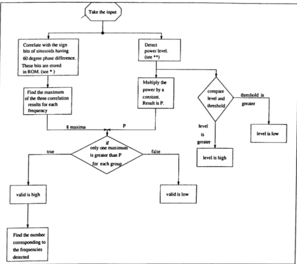
In the approach proposed in this thesis; as Proudfoot has proposed, the in­ put signal is first multiplied by the sign-bits stored in the ROM , then a number of products are added. This number is chosen according to the specifications of the detector. A power detector h«is also been added to the circuitry. This

Figure 2.7: Flow chart of the detection algorithm. (* is shown in Fig. 2.21, and ** is shown in equation 2.9)

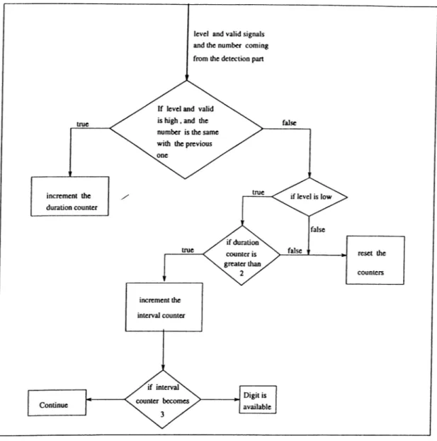
Figure 2.8: Flow chart of the decision algorithm.

is because the receiver would receive signals having amplitudes different from 1. The whole algorithm is shown by the flow charts Fig. 2.7 and Fig. 2.8. The general view of the detector is shown in Fig. 2.9.

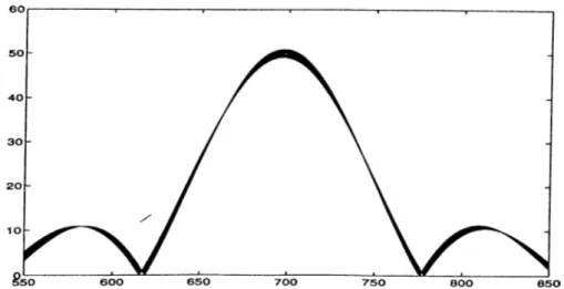
The results of the different approaches to the correlation receivers are shown in Fig. 2.10. The input is a pure sinusoid with frequency running from 550Hz to 850Hz. Correlation stands for the usual method of correlation. The input is correlated with the sinusoids

sin(27T fot)

and

cos {2wfot).

Figure 2.9: The receiver block diagram.

Figure 2.10: Frequency response for the different algorithms.

where t runs from —49.5/8000 to 49.5/8000; there are total of 100 samples for each sinusoid.

In figures Fig. 2.11, Fig. 2.12, and Fig. 2.13 the input is

sin(2?r f t + 4>)

where the frequency runs from 550Hz to 850Hz while the phase term runs from 0 to If. In method proposed by A.D. Proudfoot, the input is correlated with the hardlimited versions of sinusoids.

sign(sin(2Tr/oi))

Figure 2.11: Frequency response for the conventional correlation receiver.

Figure 2.12: Frequency response for the algorithm proposed by Proudfoot.

Figure 2.13: Frequency response for our algorithm.

and

sign(cos(27r/oi))·

In the method proposed in this thesis the input is correlated with the signals:

sign(sin(27r/o<)) sign(sin(2Tr/oi + t/ 3))

sign(sin(27r/o< + 27t/3)).

The second approeCch [10], using the binary signals for the correlation, is comparable to the approach in this thesis in area requirements. Their perfor­ mances are compared in Fig. 2.14, Fig. 2.15, Fig. 2.16 and Fig. 2.17 where the outputs of the correlators of the two approaches are shown.

In Fig. 2.14 and Fig. 2.15 the responses to the input sin(2Tr/i + <f>)\ where / runs from 500 Hz to 1100 Hz, while the phase term (j> varies from 0 to tt, are shown. In each figure there are two graphs showing the upper and lower limits for the frequency response due to the changes in phase. The lengths of the correlation windows are comparable. The correlation window length is chosen to be 100 throughout the whole thesis. The length used for the simulations of the algorithm proposed in [10] is 128.

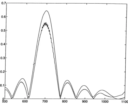
In Fig. 2.16 and Fig. 2.17 the responses of the same correlators to the input sin(27r/i + (f>), where this time / runs from llOOHz to 1800Hz, are shown. The phase is again varying from 0 to tt. It can be seen from the graphs that the sensitivity of the first correlator, which is proposed in this thesis, to high frequencies is less than the corresponding correlator.

2.3

How The System is Built

There are two main parts of the circuit (See figures Fig. 2.9, Fig. 2.18, and Fig. 2.19).

• Detection circuitry • Decision circuitry

Figure 2.14: Output of the first correlator. (Low frequencies)

Figure 2.15: Output of the corresponding correlator in [10] for the same inputs.

Figure 2.16: Output of the first correlator. (High frequencies)

0.25

0 .1 5

-0.05

flOO 1200 1300 1400 1500 1600 1700 1800

Figure 2.17: Output of the corresponding correlator in [10] for the same inputs.

Figure 2.18: Frequency detection.

2.3.1

Detection Circuit

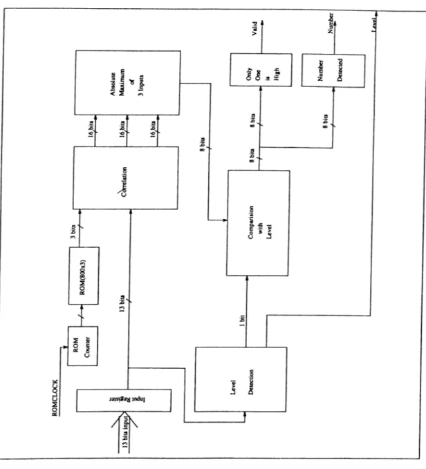
In this part of the circuit the frequency components of the input signal is mul­ tiplied with the data stored in ROM. ROM contains the sign-bits of sinusoids having the desired frequencies (697,770,852,941 and 1209,1336,1477,1633 Hz.). Three different phases for each frequency are used. The frequency values giving the maximum product is found for low group and for high group. This product and the power are proportional to the amplitude of the sinusoids. Detection block diagram is shown in Fig. 2.18.

13

c

Figure 2.19: Decision Block Diagram.

2.3.2

Decision Circuit

In detection circuit the frequencies having the greatest components are found.In decision part the signal is decided to be correct tone or not. This is done using the properties of the valid tones. (See Table 2.2). The duration of tone should be at least 40 milliseconds, and a pause longer than 30 milliseconds should follow. Fig. 2.19 shows the decision block diagram.

Figure 2.20: Phases

2.4

Algorithm

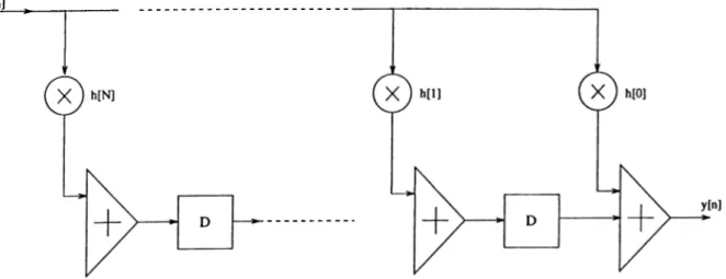
In this receiver the input stream is multiplied by 24 different bits stored in ROM (at each time step). As the multiplier is one-bit the multiplication is simple. Each product is added to the value at the output of the accumulator.

ROM contains 2400 bits (100 bits for each sinusoid). There are 3 sinusoids of each frequency:

sin(27r/t)

sin(2Tr/t + 7

t

/ 3)

sin(27T

f t

+ 27

t

/3)

The phase relations are shown in Fig. 2.20. Dashed lines show phases that are

7

T greater and sines have negative sign. The next step is taking the absolute value of the accumulated values and finding maximum of the three outputs. Fig. 2.21

The result here is the maximum of n - 1 ^ x(m ) · zi(m ) m =0 n - 1 x(m) · zi(m ) rn=0 n - 1 ^ x(m ) · zi(m ) m = 0 22

Figure 2.21: Multiplication and accumulation

where zi(m ),Z

2

(m ),Z

3

(m) are the obtained by sampling sign(sin(27r/i)) , sign(sin(27r/i + f )) and sign(sin(2Tr/i + ^ ) ) respectively, n is the length of the stream to be summed up. x is the input.

The dependency of the result on the frequency is shown in section 4.1 and the dependency of the result on the pheise of the input signal is presented in section 4.2.

Maximum value for absolute values of these three results is obtained. Then there are 8 sums to be processed; 4 for the high group of frequencies and 4 for the low group of frequencies. These sums are compared with the data coming from the power section. For a valid DTMF tone, only one of the absolute sums is greater than the power data for each group. If zero or more than one of the sums are greater than the power data, the signal is rejected. The data coming from the power section is a constant times the absolute sum of the input for the same 100 samples.

P = c - y '| x ( 0 l (2.9)

1=0

This approach is used in [10] for compensating the level difference between

input and the signal to be correlated with.

For every 100 samples this process goes on. From table 2.2 it can be seen that the duration of a valid DTMF tone is more than 40 milliseconds which corresponds to 320 samples. Tones with duration smaller than 24 milliseconds (or 23 milliseconds) should be rejected and this corresponds to 192 samples. In this detection algorithm 320 means 3 valid signals for a valid tone. The minimum duration that can pass this 3 consecutive valid pulse specification is 250 samples. After 3 consecutive valid pulses, there should be 3 consecutive silence pulses (similar^irgument). When 3 valid pulses are followed by 3 silence pulses the DTMF tone is accepted.

Chapter 3

IMPLEMENTATION

The DTMF receiver proposed is implemented in ES2 CMOS 1/r technology using Cadence Environment, which makes possible to develop the design hier­ archically. First the schematics of the implementation is drawn using standard cells, then the layout is obtained using standard place and route algorithms of the software. In this chapter the realization of the design is explained.

The first hierarchy level of the digital DTMF receiver includes the following subblocks:

• Detection of the Frequencies • Decision

The cells used to implement the whole circuit are shown in tables 3.1 and 3.2.

The clock is chosen to be 1024 kHz.

3.1

Detection Circuit

The input is taken, it is correlated with the ROM data and a guess for the input frequency is done in the detection part.

cell name includes description topp ^ o p l and pads top schematic with pads topi detectcell declog2 multiplexors top circuit detectcell testpow eightzeros corrcelnew powlev level2 fmaxdownl6 outreg2 down8003 outnum outreg findmax onlyone equalreg cmpwithlev compclk rom comparât downl6 ckdivS inreg

detection part of the circuit

comparât comp3 comp3 abs2 maxof3

Table 3.1: Cells in the hierarchy of the DTMF receiver circuit

celKname included cells description rom downSOO romSout rom corrcelnew muxedregmat corr andarr Correlation muxedregmat muxedreg powlev testpow comparator levdownl28 abssummer levelreg Signal Level Detection comparator compcell comp cell compcella

compcellb abssummer countlOO andarr corr levelreg div declog2 eff durcount2 intcount2 sysdata cmp Decision

Table 3.2: Cells in the hierarchy of the DTMF receiver circuit

The input is latched into the register block inreg. IMHz clock is divided by 128 and input is latched with the rate of 8 kHz. The clocking blocks for this division are downl6 and ckdivS. First one divides by 16, and second divides by 8. 1 MHz clock is for shifting data serially.

Then the output of the register is fed to level detector and correlators.

3.1.1

Correlators

Actually there are 24 adders needed for correlators. Instead of using 24 adders, 3 adders are used and the rate of the input taken is 8 times larger. Here, three adders are preferred to a single adder with an input rate 24 times larger because the available clocks have the rate of a power of 2.

Input is multiplied by the bit coming from the ROM, the result is added to the output of a register matrix and result is shifted into the same matrix again. (Block diagram is in Fig. 3.1). Schematic of the correlator is in Appendix B.l

Each correlation block has one 20-bit adder and a register matrix for storing the sums (20 bits by 8). 3 correlation blocks performs the correlation with 3 different phases respectively. (And can be expanded to 4 or more with small changes in the next stage).

Corrcelnew is the hierarchy name for the correlation block containing the correlator,register matrix -muxedregmat-, and andarr for masking the output. This masking is needed to clear the sum for every 100 samples. This meisking signal is obtained from a synchronization pulse generated at the ROM block.

3.1.2

R O M

Rom is the section for generating the sign bits of sinusoids sin(2Tr/<), sin(

27

r /t -f- 7t/ 3) and sin(2Tr/< + 2;r/3). This block is generated with the syn­ thesis tool of Cadence. At every time step three sign bits are generated and the frequency is changed from the highest one to the lowest one. The time step here is 1/8 of the input period.i.e. rate is 8 times the input frequency. The 1 MHz clock is divided by 16 and the clock for the ROM is generated. The same clock is used to shift the contents of the register matrix.

20 bits

REGISTER MATRIX

Figure 3.1: The correlator block diagram.

3.1.3

Level Detection

The schematics related to level detection are in Appendix B .l. It sums the absolute value of the input data for every period of 100 samples. The absolute sum is calculated with a similar way to the correlation. The same input is taken but here the sign bit of the signal is used as multiplier instead of the bit coming from the ROM. i.e., if the input data is positive it is added to the sum; otherwise it is subtracted from the sum.

In the comparator block the level is compared to the smallest allowable level. It is a 20 bit comparator and it is an entirely combinational circuit. In figures 3.2, 3.3 and 3.4 there is a 2-bit comparator. 20-bit comparator is obtained by cascading this cell. If A is high output Cout is logic-1; if B is large output Dout is logic-1 else both outputs are logic-0.

Levdownl28 is the frequency divider. As its name indicates it divides by 128. (used clock is 8 kHz).

Levelreg block multiplies the power value by a constant which can be se­ lected by choosing Si and SO. (Table 3.3) This multiplication is done by choosing 1/4 or 1/2 or 1/8 of the input value and adding to another one. This

SO SI m u ltip lier

0 0 3/8

0 1 1/2

1 0 5/8

1 1 3/4

/ Table 3.3: The multiplier

result is converted into serial data. Only the first 16 bits are used.

3.1.4 Comparison of three phases

This comparison is performed serially. As it can be seen in the Fig. 3.5 first the absolute value of the 3 numbers are calculated. If the sign bit is positive the serial data appear at the output, otherwise the inverse of every bit exists at the output serially. The calculated value is 1 lower than the absolute value of the number for negative inputs. But this was preferred for the sake of smaller area. The positive numbers are then latched into the maxofS subblock. The first two serial inputs are compared serially in the first clock period then the larger one is compared with the other one in the next clock period.

The results are compared to the serial output coming from the level detec­ tion block at the cmpwithlev block. This performs the same algorithm with the previous comparator. (Fig. 3.7)

3.2

Decision Circuit

In this section of the circuit it is decided that if the input stream defines a DTMF signal or not. The implemented schematic of Fig. 2.19 is in Fig. 3.8

There are 4 important blocks in the decision part.

• Duration counter: durcount • Interval counter: intcount

< Cin C ou tb c o c n p c e llb Din D outb iQ i i m cmpb < Dinb c o o ç > c e lla C out GQ Dout

Figure 3.2: two-bit comparator

Figure 3.3: subblock compcella.

Figure 3.4: subblock compcellb.

Figure 3.5: The absolute comparison of three inputs.

• Comparison of the previous and current numbers: cmp • Output converter into system data isysdata

3.2.1

Duration and Interval Counter

Duration counter starts counting when the previous and the current numbers are equal. This means that the signal with the same frequency components is continuing. Otherwise the counter is always zero. It stops counting when counter reaches 2. (That is three samples are the same).

Interval counter starts counting when the duration counter is 2 and the signal level is low.(i.e. pause). It counts from 1 up to 4 and stops at 4. when signal level becomes high it returns back to its initial value 1.

3.2.2

Comparison

This block compares the previous and the current numbers. This comparison is performed by a simple subtraction. If all the bits become zero, the output changes from 0 to 1.

Figure 3.6: Circuit giving the maximum of three inputs.

Figure 3.7: Comparison with level.

1!

Figure 3.8: Decision circuit schematic 35

il. •H i: □ IF >9* T~* 17. l i

Figure 3.9: The duration counter.

3.2.3

System Data

This block converts the decided number into a form that the microprocessor will understand. This subblock is generated by the help of the Synthesis tool of Cadence. Input output relation can be seen in Table 3.4. At the input side the leftmost two bits represent the low frequencies and the rightmost two bits represent the high frequencies.

Figure 3.10: The interval counter.

button in out

1

0000

0001

2

0001

0010

3

0010

0011

4

0100

0100

5

0101

0101

6

0110

0110

7

1000

0111

8

1001

1000

9

1010

1001

0

1101

1010

*

1100

1011

#

1110

1100

A

0011

1101

B

0111

1110

C

1011

n il

D

n il

0000

Table 3.4: Conversion Map

Chapter 4

SIMULATION RESULTS AND

TESTING THE

IMPLEMENTATION

In the design step, the frequency and phase dependence are examined by using Matlab simulations. Then the decision logic is developed by using C-language. In this chapter, the results of these simulations are explained and the additions for test purposes are described.

4.1

Frequency Dependence

Actually there are 24 filters used here, each of which is tuned to a different frequency. Also every correlator has different responses to the inputs having different phases. In Fig. 4.1, the outputs of the correlations with

sign(sin(2Tr697t)

sign(sin(2Tr697i + 7r/3) sign(sin(2Tr697< + 27t/3 )

are shown. Here the input is cos(27tf t ) where the input frequency / runs from 500Hz to lOOOHz. The next figure (Fig. 4.2) shows absolute values of the same outputs for the same input. The second graph in the same figure shows the

Figure 4.1: Frequency dependence of the first three correlators

absolute values of the same correlator outputs for input signals cos{2rft + <f>) where / runs from 500Hz to 800Hz and <j) runs from 0 to tt.

In Fig. 4.3 the outputs of all the correlators are shown. The peaks corre­ spond to the correlators tuned to the frequencies belonging to the low group. (Centers are located at 697,770 852,952 Hz). In this figure, the input frequency runs from 550 to 1100 Hz. The larger values (peaks) are the responses of the correlator nearest to the input frequency. In Fig. 4.4 the outputs of all the correlators are shown. The peaks correspond to the correlators tuned to the frequencies belonging to the high group. (Centers are located at 1209, 1336, 1477, 1633 Hz). The input frequency runs from 1100 to 1800 Hz. The shaded regions are because of the different phases (i.e. 0 to tt) used at the input.

In Fig. 4.5 output of the absolute maximum for the input cos(27r/t -f- <j>). ( / = 1150..1700 Hz and <f> = 0..7t) is shown.

The next figure (Fig. 4.6 shows the frequencies that should be rejected or accepted. The regions between rejected and accepted are the tolerance regions which include the frequencies that can be either accepted or rejected.(It is

Figure 4.2: Frequency dependence of the first three correlators

700 800 900 frequency (Hz)

1000 1100

Figure 4.3: Outputs after the absolute maximum (low group)

70r

1100 1200 1300 1400 1500 1600 1700 1800 frequency (Hz)

Figure 4.4: Outputs after the absolute maximum (high group)

Figure 4.5: Frequency dependence of the 7’th three correlators

similar for the other correlator outputs)

4.2

Phase Dependence

Because 3 correlators with 60 degrees phase difference are used, the phcise difference of the input with one of the correlating signals are 30 degrees at most. Because of this the width of the shaded regions in the previous figures is narrower than with correlations with sine and cosine.(7r/2 phase difference). Figure Fig. 4.7 shows the phase dependence of the output at the 6th correlation output.

4.3

Simulation Results

After simulations it is seen that the receiver satisfies the specifications of CCITT. Some simulations for the frequency tolerances are made by the help

1400 1420 1440 1460 1480 1500 1520 1540 1560 frequency (Hz)

Figure 4.6: Frequency dependence of the seventh three correlators

of C programming language, and MATLAB. The results of these simulations are given in Table 4.1.

In Table 4.1, it can be seen that the frequency tolerance for low group frequencies is group frequencies it is responses are more steep for the high group.

4.4

Testing the Design

Testing is the problem of determining, in a cost effective way, whether a chip, module, board or system has been manufactured correctly. Increasing circuit complexities increase the cost of testing. To reduce this cost a collection of techniques known as ’’ Design For Testability (D F T )” is carried on (Making internal nodes in a circuit more accessible; transforming sequential circuits into combinational circuits, or decomposing complex circuits into less complex sub-functions for the purposes of testing reducing the amount of test data which is needed to test the circuit). The main thing is to insert a reset into all

Figure 4.7: Phase dependence of the sixth correlation (labels in degree)

low frequency tolerance high fre-quenc toler­ ance -%5 -%3 -%2 exact %2 %3 %5 -%5 ND ND ND ND ND ND ND -%3 ND ND ND ND ND ND ND -%2 ND D D D D D ND exact ND D D D D D ND %2 ND D D D D D ND %3 ND ND ND ND ND ND ND %5 ND ND ND ND ND ND ND

Table 4.1: Response of the system for different input freq uencies. (ND : not detected; D : detected).

digital systems, this has the advantage of starting all states from known values. In this chip, in order to function properly the system should begin from zero, and all internal nodes are set to a value.

This chip will be in fact used as a part o f a telecommunication chip. The full testing circuitry has not been designed yet. But this chip contains some separate circuits for testing. For level detection testpow is designed. It takes the value, converts it into serial data and shifts it to the output.

Other outputs of the subblocks are also multiplexed and connected to the output pads (Fig. 4.8). This is for making more nodes observable at the output.

For selecting the bits at the multiplexer inputs 3 select signals are intro­ duced. SOTest, Si Test and S2Test. These select signals choose 4 of 24 inputs including level, level data, comparator outputs, correlations, ROM outputs, valid and level signals, counter outputs and clocks generated.

ii]

Figure 4.8: top schematic including the multiplexors for test

Chapter 5

CONCLUSIONS

In this thesis, a new implementation of a single chip digital DTMF receiver is explained.

Different from usual correlation receivers using 2 correlations with the func­ tions having 7t/ 2 phase difference, 3 correlations with 7r/3 phase difference is used. This has been done in order to reduce the errors coming from taking maximum instead of squaring and adding. These errors make it difficult to choose a threshold. The maxima of the results of these correlations are found instead of squaring and adding to decrease the area requirements and circuit complexity. Also, an approximate power detector is added to decrease false alarm rate.

The correlation part of the detector can be used in other detectors as it does not include any multiplication which increases the complexity. The im­ plementation is simpler as well.

The simulations of design are done by using Matlab and C-programming language. Design is implemented in Cadence -Design Framework II- environ­ ment and simulated by Verilog simulator.

The designed chip is in ES2 l-//m CMOS technology. It is 4.802 mm by 5.161 mm having a total area about 24.78mm^. The registers and correlators require the largest area, 6.2mm^, where core area is 16.3mm^. It has 40 pins in­ cluding 4 ground and 4 supply pins. It contains 3787 cells and 58259 equivalent transistors.

REFERENCES

[1] Martin P. Clark. Networks and Telecommmunications. John Wiley & Sons, Inc., 1991.

[2] A. Michael Noll. Introduction to Telephones and Telephone Systems. Artech House, 1986.

[3] William Sinnema and Tom McGovern. Digital, Analog, and Data Com­ munication. Prentice Hall Inc., second edition, 1986. Chapter 2 and 3. [4] George Gara Ivan Koval “Digital MF receiver using discrete fourier trans­

form,” IEEE Transactions on Communications, vol. COM-21, December 1973.

[5] JR. Michael J. Callahan “ Integrated dtmf receiver,” IEEE Journal of Solid-State Circuits, vol. SC-14, pp. 85-90, February 1979.

[6] George F. Landsburg Bertram J. White, Gordon M. Jacobs “ Monolithic dual tone multi frequency receiver,” IEEE Journal of Solid-State Circuits, vol. SC-14, pp. 991-997, December 1979.

[7] J. Tow J. R. Boddie, N. Sachs “Receiver for TOUCH-TONE service,” The Bell System Technical Journal, vol. 60, pp. 1573-1583, September 1981.

[8] Fritz G. Braun “Nonrecursive digital filters for detecting multifrequency code signals,” IEEE Transactions on Acoustics, Speech and Signal Pro­ cessing, vol. ASSP-23, pp. 250-256, June 1975.

[9] J.N. Denenberg “Spectral moment estimator: A new approach to tone detection,” The Bell System Technical Journal, vol. 55, pp. 143-155, February 1976.

[10] Theo A. C. M, Claasen and J. B. H. Peek “ A digital receiver for tone detec­ tion applications,” IEEE Transactions on Communications, vol. COM-24, December 1976.

[11] David Agnew “Simplified tone detector for pcm channel,” IEEE Transac­ tions on Acoustics, Speech and Signal Processing, vol. ASSP-31, pp. 8-16, February 1983.

[12] A.D. Proudfoot “Simple multifrequency-tone detector,” Electronic Let­ ters, vol. 8, pp. 524-525, October 1972.

[13] Pieter Eijkhoff. System identification : parameter and state estimation. Wiley-Interscience, 1974. section 8.3, pages 299-302.

[14] Yoshihito Haneda Yoshiaki Tadokoro “Dual tone multifrequency receiver using synchronous additions and subtractions,” IEEE Transactions on

Communications, vol. COM 35, pp. 414-418, April 1987.

APPENDIX A

SOURCE FILES

A .l

Algorithm Implemented

#include <stdio.h> #include <math.h>

#define max(a,b) ((a)>(b) ? (a) : (b))

#define max3(a,b,c) max(a,max(b,c)) #define NUM 100 #include </maJiisah/ee/ekinci/dtmfrec/cflies/coralg/save.h> char digit[4][4]; int sign(x) double x; { if (x >= 0) return(l); else return(-l); } int findnum(number) int number[]; { int i,flagl,flag2,ret; ret = flagl=flag2=0; 51

for(i=0;i<4;i++){ if (number[i]>0) { flagl = flagl + 1; ret = 10*(i+l); } } for(i=4;i<8;i++){ if (number[i]>0) { flag2 = flag2 + 1; ret = ret + i - 3; } }

if ((flagl ==1) && (flag2 == 1))

return(ret) ; else return(-l); } detect(x,y,N) double **x,**y; int N; { int level,i,j.durcount,intcount,numnow,numpast,indexl,index2; int number[8]; numnow = numpast = -1; for (i = 0;i<N;i++){ if (x[i][0]>2000) level = 1; else level = 0; if (level > 0){ for (j = 0;j<8;j++H

numberCj] = ((y[i] [j]>(x[i] [0]*4/8)) ? 1:0);

} intcount = 0; numnow = findnum(number); if (i > 0) if (numpast != -1){ indexl = (int)(numpast/10)-l; index2 = (numpast */, 10) + 3; if ((y[i][indexl]< (y[i-1][indexl]*3/4))

I I

(y[i][index2]<(y[i-1][index2]*3/4))) { 52

level = 0; numnow = numpast; } } if ((level > 0)&&(nunmow != -1)){ if (numnow == numpast) durcount = durcount +1; else durcount = 0; } if (numnow == -1) durcount = 0; } if (level == 0){ if (durcount >=2) intcount = intcount + 1; indexl = (int)(numnow/10)-l; index2 = (numnow Y, 10) -1; if (intcount==3)

printfC'at point */,d number */,c is detected \n", i.digit[indexl][index2]); } printf("%d\n",level); numpast = numnow; main(arge, argv) int arge; char *argv[]; {

char *fnamel, *fname2, *fname3, *fncune4;

int i, j, test[24][NUM], N1, N2, N3, noofinp.inc.savinp;

float input;

double inp, dummy;

FILE *fopen(), *fl, * f 2 ; double freqs[8]; double * * z , ♦*zt,**zmax; double **res; double t[NUM]; if (argc != 2) exit(1); fl = fopen(argv[l], "r");

fneimel = (char *)calloc(10, sizeof (char)); fname2 = (char *)calloc(10, sizeof(char)); fnameS = (char *)calloc(10, sizeof(char)); fname4 = (char *)calloc(10, sizeof(char)); fnamel = "z"; fnaitie2 = "ztest"; fnajneS = "level"; fname4 = "zmaix"; digit [0][0] = '1' digit [0][1] = '2' digit[0][2] = '3' digit [0][3] = 'A' digit [1][0] = ’4' digit[l] [1] = '5' digit[1] [2] = '6' digit [1][3] = 'B’ digit[2][0] = '7' digit[2][1] = '8' digit[2][2] = '9' digit[2][3] = ’C ’ digit [3][0] = digit [3][1] = ’0 ’ digit[3][2] = '#' digit [3][3] = 'D'

scanf ("*/,d" , ftnoof inp) ;

scanf ("*/,d" ,&savinp) ; N1 = noofinp;

N2 = 24;

N3 = (int)(Nl/100)+l;

res = (double **)calloc(N3,sizeof(double *));

for (i=0; i < N3;i++)

res[i] = (double *)calloc(l,sizeof(double)); z = (double **)calloc(Nl, sizeof(double * )); for (i = 0; i < N1; i++)

z[i] = (double *)calloc(N2, sizeof(double)); zmax = (double **)calloc(N3,sizeof(double *)); for (i = 0; i < N3; i++)

zm2Lx[i]

= (double *)calloc(8,sizeof (double)) ;

zt = (double **)calloc(NUM, sizeof(double * )); for (i = 0; i < NUM; i++)

zt[i] = (double *)calloc(N2, sizeof(double));

freqs[0] = 697; freqsCl] = 770; freqs[2] = 852; freqs[3] = 941; freqs[4] = 1209 freqs[5] = 1336 freqs[6] = 1477 freqs[7] = 1633;

for (i = 0; i < NUM; i++)

t[i] = i - (NUM - 1) / 2.0;

for (i = 0; i < 8; i++) {

for (j = 0; j < NUM; j++) {

dummy = sin(2 ♦ M_PI * t[j]* freqs[i] / 8000.0); test[i][j] = sign(dummy);

dummy = sin(2 * M_PI * t[j] * freqs[i] / 8000.0 + M_PI / 3.0);

test[i+8][j] = sign(dummy);

dummy = sin(2 * M_PI * t[j] * freqs[i] / 8000.0 + 2 ♦ M_PI / 3.0); test[i+16][j] = sign(dummy); } } inc = -1 ; 55

for (i = 0; i < N1; i++) { fscanf(fl, ftinput) ; if ((i ·/. 100) == 0){ inc = inc + 1; res[inc][0] = fabs(input); for (j = 0; j < 8; j++) {

z[i][j] = input * (testCj] [0]); z[i][j+8] = input ♦ (test [j+8] [0] ) ;

z[i][j + 16] = input * (test[j + 16] [0]) ;

} }

else{

res[inc] [0] = res[inc][0] + fabs(input); for (j = 0; j < 8; j++) {

z[i][j] = z[i-l][j] + input * (test [j] [i’/.NUM] ) ;

z[i][j+8] = z[i-l][j+8] + input *

(test [j+8][i’/.NUM]);

z[i][j+16] = z[i-l][j + 16] + input ♦

(test [j+ 16] [i*/.NUM]); } } } for (i = 0; i < (N3 -1); i++){ for(j = 0; j <8;j++){ zmax[i][j] = max3(fabs(z[i*100+99] [j]) , fabs(z[i*100+99] [j+8]) , fabs(z[i*100+99] [j+16])) ; } detect(res,zmax,N3); if (savinp != 0){ save_array(z, N1, N2, fnamel); for (i = 0; i < NUM; i++)

for (j = 0; j < N2; j++) {

zt[i][j] = (double)test[j] [i] ;

}

save_array(zt, NUM, N2, fname2);

save_array (res ,N3,1, fnaimeS) ; save_array(zmax, N3,8, fname4); }

A .2

Frequency and Phase Dependence

A .2.1

C-file

#include <stdio.h> #include <math.h> # include <malloc.h> »include "/manisali/ee/ekinci/dtmfrec/cfiles/coralg/save.h" »define NUM 100 int sign(x) double x; if (x >= 0) return(1); else return(-1); }

inputsin(amp, freq, phase, inp)

double amp, freq, phase;

double inp[NUM];

{

int i;

double phi;

phi = phase * M„PI / 180.0;

for (i = 0; i < NUM; i++) {

inp[i] = amp ♦ cos(2 * M_PI * freq * i / 8000 + phi);

} main(arge, argv) int arge; ehar *argv[]; { double double double double int dummy; **z;

freqs[8], inpfre, firstfre, lastfre, stepfre; inpphi, firstphi, lastphi, stepphi;

j, test[24][NUM], indexfre, lenfre, indexphi, lenphi, index;

double t[NUM];

double input[NUM];

ehar *fneimel;

fnamel = (ehar *)ealloe(10, sizeof(ehar));

seaixf ("*/,lf ", &firstfre) ; seanf("*/.lf", ftlastfre); s e a n f C U f " , ftstepfre); seanf ("*/.lf", ftfirstphi); seauf("'/,lf", ftlastphi); seanf("'/,If", ftstepphi);

lenphi = (int)((lastphi - firstphi) / stepphi + 1); lenfre = (int)((lastfre - firstfre) / stepfre + 1); z = (double **)ealloe(24, sizeof(double ♦ ));

for (i = 0; i < 24; i++)

z[i] = (double *)ealloe(lenfre ♦ lenphi, sizeof(double));

fnamel = argv[l]; freqs[0] = 697; freqs[l] = 770;

freqs[2] freqs[3] freqs[4] freqs[5] freqs[6] freqs[7] 852; 941; 1209 1336 1477 1633

for (i = 0; i < NUM; i++) /* Time -49.5/8000 to 49.5/8000 ♦/

t[i] = i - (NUM - 1) / 2.0;

for (i = 0; i < 8; i++) {

for (j = 0; j < NUM; j++) {

dummy = sin(2 * M_PI * t[j] * freqs[i] / 8000.0); test[i][j] = sign(dummy);

dummy = sin(2 * M_PI * t[j] ♦ freqs[i] / 8000.0 +

M_PI / 3.0);

test[i+8][j] = sign(dummy) ;

dummy = sin(2 * M_PI * t[j] * freqs[i] / 8000.0 + 2 ♦ M_PI / 3.0);

test[i+16][j] = sign(dummy);

} }

for (inpphi = firstphi; inpphi <= lastphi; inpphi = inpphi + stepphi) {

indexphi = (int)((inpphi - firstphi) / stepphi); for (inpfre = firstfre; inpfre <= lastfre;

inpfre = inpfre + stepfre) {

inputsin(l.0, inpfre, inpphi, input);

indexfre = (int)((inpfre - firstfre) / stepfre); index = indexphi * lenfre + indexfre;

for (j = 0; j < 24; j++) z[j] [index] = 0;

for (i = 0; i < NUM; i ++) { for (j = 0; j < 8; j++) {

z[j] [index] = z[j] [index] + input [i] * (test[j] [i]);

z[j+8] [index] = z[j+8] [index] + input [i] ♦