WAVE SCATTERING FROM DIELECTRIC
RANDOM ROUGH SURFACES
a thesis
submitted to the department of electrical and
electronics engineering
and the institute of engineering and science
of bilkent university
in partial fulfillment of the requirements
for the degree of
master of science
By
Kıvan¸c ˙Inan
Asst. Prof. Vakur B. Ert¨urk (Advisor)
I certify that I have read this thesis and that in my opinion it is fully adequate, in scope and in quality, as a thesis for the degree of Master of Science.
Prof. Dr. Ayhan Altınta¸s
I certify that I have read this thesis and that in my opinion it is fully adequate, in scope and in quality, as a thesis for the degree of Master of Science.
Assoc. Prof. Sencer Ko¸c ii
Prof. Dr. Mustafa Kuzuo˘glu
I certify that I have read this thesis and that in my opinion it is fully adequate, in scope and in quality, as a thesis for the degree of Master of Science.
Asst. Prof. Defne Akta¸s
Approved for the Institute of Engineering and Science:
Prof. Dr. Mehmet B. Baray Director of the Institute
ELECTROMAGNETIC WAVE SCATTERING FROM
DIELECTRIC RANDOM ROUGH SURFACES
Kıvan¸c ˙Inan
M.S. in Electrical and Electronics Engineering Supervisor: Asst. Prof. Vakur B. Ert¨urk
July, 2005
Mobile radio planning requires accurate prediction of electromagnetic field strengths over large terrain profiles. However the conventional method of mo-ments (MoM) becomes unsuitable for electrically large rough dielectric surfaces, because of the O(N3) computational cost due to the large number of surface unknowns N. Iterative Methods are beneficial methods for faster electromag-netic problem solutions. By using such methods, very accurate results can be achieved, causing a computational cost of O(N2). In this work, among the sta-tionary iterative methods; Forward-Backward Method (FBM), and among the nonstationary iterative ones; Conjugate Gradient Squared (CGS), BiConjugate Gradient Stabilized (Bi-CGSTAB) and Quasi Minimal Residual (QMR) Methods are presented to investigate the electromagnetic wave scattering from dielectric random rough surfaces. These techniques are compared to each other over various kinds of surface models that reflect the real terrains to find out the best solution methodologies. Furthermore, efficiency of the methods are assessed by compar-ing the obtained scattercompar-ing results, normalized radar cross sections (NRCS) of the surfaces considered, with the numerically exact ones computed by employing the MoM.
Keywords: Random Rough Surface Scattering, Method of Moments (MoM), Forward-Backward Method (FBM), Conjugate Gradient Squared Method (CGS), BiConjugate Gradient Stabilized Method (Bi-CGSTAB), Quasi Minimal Residual Method (QMR), Normalized Radar Cross Section (NRCS).
D˙IELEKTR˙IK RASGELE DALGALI Y ¨
UZEYLERDEN
ELEKTROMANYET˙IK DALGA SAC
¸ ILMASINDA
˙ITERAT˙IF Y ¨ONTEMLER˙IN UYGULAMALARI
Kıvan¸c ˙Inan
Elektrik ve Elektronik M¨uhendisli˘gi, Y¨uksek Lisans Tez Y¨oneticisi: Asst. Prof. Vakur B. Ert¨urk
Temmuz, 2005
Mobil radyo planlaması geni¸s y¨uzey yapılarında elektromanyetik alan kuvve-tinin do˘gru tahminini sa˘glamaktadır. Ancak klasik moment y¨ontemi, (MoM), y¨uzey bilinmeyenleri ¸cok fazla oldu˘gu zaman, ¸c¨oz¨umleme y¨uk¨un¨un O(N3) masından dolayı ¸cok dalgalı ve elektriksel olarak geni¸s y¨uzeylerde uygun ol-mamaktadır. ˙Iteratif yakla¸sımlar, elektromanyetik problemlerin daha hızlı ¸c¨oz¨umlemeleri hususunda olduk¸ca etkilidir. Bu y¨ontemler kullanılarak, ¸c¨oz¨um y¨uk¨u O(N2) olan ¸cok do˘gru sonu¸clar elde edilebilir. Bu tezde, sabit iter-atif y¨ontemlerden ˙Ileri-Geri Metodu ve sabit olmayan iteriter-atif y¨ontemlerden Kısmen Minimum Kalan, Bi-E¸slenik Gradyan Stabil ve E¸slenik Gradyan Kareli y¨ontemlerinin dielektrik rasgele dalgalı y¨uzeylerdeki elektromanyetik dalga sa¸cılmaları uygulamalarına yer verilmi¸stir. Ayrıca bu ¸c¨oz¨umleme teknikleri, en iyi ¸c¨oz¨umleme metodolojilerini ifade etmek i¸cin ger¸cek y¨uzeyleri yansıtan bir¸cok pro-fil i¸cin kar¸sıla¸stırılmı¸stır. Bunlarla birlikte bu tezde kullanılan iteratif y¨ontemlerin ba¸sarısı ve do˘grulu˘gu, y¨ontemler vasıtasıyla elde edilen normalize edilmi¸s radar kesit alanlarının, numerik olarak kesin sonu¸c olan MoM’un uygulanmasıyla bulu-nan normalize edilmi¸s radar kesit alanlarıyla kar¸sıla¸stırılarak de˘gerlendirilmi¸stir.
Anahtar s¨ozc¨ukler : Rasgele Dalgalı Y¨uzey Sa¸cılması, Moment Y¨ontemi, ˙Ileri-Geri Y¨ontemi, Kısmen Minimum Kalan Y¨ontemi, Bi-E¸slenik Gradyan Stabil Y¨ontemi, E¸slenik Gradyan Kareli Y¨ontemi, Normalize Edilmi¸s Radar Kesit Alanı.
I would like to express my sincere gratitude to Dr. Vakur B. Ert¨urk for his supervision, guidance, suggestions, instruction and encouragement through the development of this thesis.
I would like to thank to Dr. Ayhan Altınta¸s, Dr. Sencer Ko¸c, Dr. Mustafa Kuzuo˘glu and Dr. Defne Akta¸s for reading the manuscript and commenting on the thesis.
I would like to thank to Dr. Antonio Iodice for his suggestions and guidance who has answered with patience all of my questions about his published articles. Finally, I would like to express my appreciation to my parents, and my brother for their endless love and continuous support throughout my life.
1 Introduction 1
1.1 Literature Survey . . . 2
1.2 Scope and Contributions of the Thesis . . . 4
1.3 Outline of the Thesis . . . 5
2 Background 6 2.1 Integral Equation Formulation For Dielectric Surfaces . . . 6
2.1.1 General Equations for Electromagnetic Fields with Electric and Magnetic Sources and Boundary Conditions . . . 6
2.1.2 Physical Problem . . . 10
2.1.3 Equivalent Problem for Region 1 . . . 11
2.1.4 Equivalent Problem for Region 2 . . . 14
2.1.5 Surface Integral Equations for Equivalent Surface Currents 16 2.2 Random Rough Surface Generation . . . 19
2.2.1 Gaussian Spectrum . . . 24
2.2.2 Exponential Spectrum . . . 25
2.3 Method of Moments . . . 27
2.3.1 Computational Considerations . . . 28
2.3.2 Basis Functions . . . 29
2.3.3 Weighting Functions . . . 29
3 Solution for the Problem 31 3.1 HH Polarization . . . 33 3.2 VV Polarization . . . 37 3.3 Solution Procedure . . . 40 4 Iterative Algorithms 41 4.1 Stationary Methods . . . 42 4.1.1 Forward-Backward Method . . . 42 4.2 Nonstationary Methods . . . 47
4.2.1 Conjugate Gradient Method [36] . . . 47
4.2.2 BiConjugate Gradient Method [36] . . . 50
4.2.3 Conjugate Gradient Squared Method [36] . . . 52
4.2.4 BiConjugate Gradient Stabilized Method [36] . . . 54
4.2.5 Quasi - Minimal Residual Method [36] . . . 57
5 Simulations and Results 62
5.1 Validation of the Algorithms . . . 63
5.2 Application of the Iterative Methods . . . 70
5.2.1 Superiority of the Nonstationary Algorithms . . . 78
5.2.2 Important Remarks . . . 82
6 Conclusions 85 6.1 Some Interesting Future Directions . . . 87
A Detailed Derivations of the Matrix Elements 88 A.1 HH Polarization . . . 88
2.1 Two media with µ1, ²1 and µ2, ²2 where both electric and magnetic current sources exist. . . 10 2.2 Physical problem describing the scattering from rough dielectric
surface . . . 11 2.3 Equivalent problem A for scattering from dielectric rough surface 12 2.4 Equivalent problem B for region 2 for scattering from dielectric
rough surface . . . 14 2.5 A small circular disk of radius a about r. . . . 17 2.6 (a)Gaussian correlated moderately rough surface with σ =
λ/6, Lc = λ, so that the rms slope is = 13◦ at 1 GHz (b)Gaussian
correlated very rough surface with σ = 0.707λ, Lc= λ, so that the
rms slope is = 45◦ at 1 GHz . . . . 25
2.7 (a)Exponentially correlated moderately rough surface with σ = λ/6, Lc = λ, so that the rms slope is = 13◦ at 1 GHz
(b)Exponentially correlated very rough surface with σ =
0.707λ, Lc= λ, so that the rms slope is = 45◦ at 1 GHz . . . 26
3.1 Geometry of scattering from dielectric random rough surface problem 31
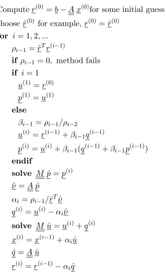
4.1 Pseudocode of the Preconditioned Conjugate Gradient Method . . 49
4.2 Pseudocode of the Preconditioned BiConjugate Gradient Method 53
4.3 Pseudocode of the Preconditioned Conjugate Gradient Squared Method . . . 55 4.4 Pseudocode of the Preconditioned BiConjugate Gradient
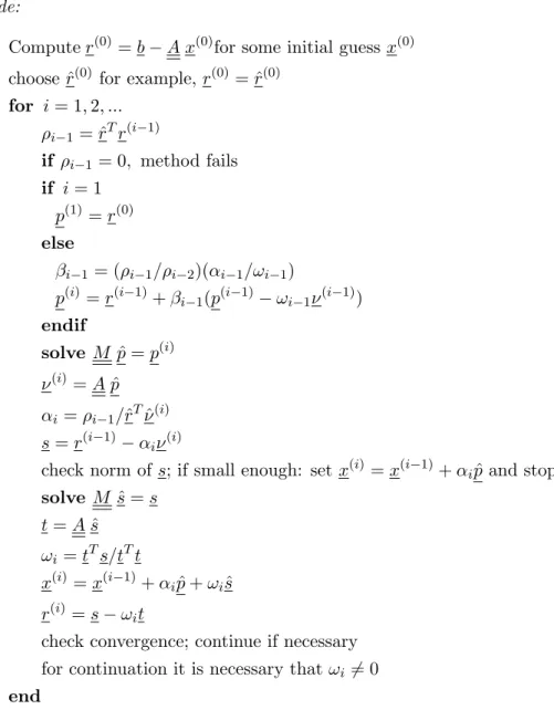
Stabi-lized Method . . . 58 4.5 Pseudocode of the Preconditioned Quasi Minimal Residual Method 60 5.1 Comparison of the monostatic NRCS values from [24] for various
angles of incidence with the results obtained in this study for a dielectric constant, ²r = 4 for HH polarization at 1 GHz. (a)σ =
λ/6, rms slope= 13◦ (i.e. moderately rough surface). (b)σ =
0.707λ, rms slope= 45◦ (i.e. very rough surface ). . . . 64
5.2 Comparison of the monostatic NRCS values from [24] for vari-ous angles of incidence with the results obtained in this study for a dielectric constant, ²r = 15 − j4 for HH polarization at 1
GHz. (a)σ = λ/6, rms slope= 13◦ (i.e. moderately rough surface).
(b)σ = 0.707λ, rms slope= 45◦ (i.e. very rough surface ). . . . 65
5.3 Comparison of the monostatic NRCS values from [24] for various angles of incidence with the results obtained in this study for a dielectric constant, ²r = 4 for VV polarization at 1 GHz. (a)σ =
λ/6, rms slope= 13◦ (i.e. moderately rough surface). (b)σ =
0.707λ, rms slope= 45◦ (i.e. very rough surface ). . . . 66
5.4 Comparison of the monostatic NRCS values from [24] for vari-ous angles of incidence with the results obtained in this study for a dielectric constant, ²r = 15 − j4 for VV polarization at 1
GHz. (a)σ = λ/6, rms slope= 13◦ (i.e. moderately rough surface).
5.5 Comparison of the bistatic NRCS values from [24] for Gaussian correlated rough profile with the results obtained in this study for a dielectric constant, ²r = 4 at 1 GHz and σ = λ/6, rms slope= 13◦
(i.e. moderately rough surface) (Angle of incidence is 75◦). (a) HH
Polarization (b)VV Polarization . . . 68 5.6 Comparison of the bistatic NRCS values from [24] for
exponen-tially correlated rough profile with the ones we have derived for a dielectric constant, ²r = 4 at 1 GHz and σ = λ/6, rms slope= 13◦.
(Angle of incidence is 75◦) (a) HH Polarization (b)VV Polarization 69
5.7 Comparison of the monostatic NRCS values for different iterative methods for Gaussian correlated rough profile with a dielectric constant, ²r = 4 for HH polarization at 1 GHz. (a)σ = λ/6, rms
slope= 13◦. (b)σ = 0.707λ, rms slope= 45◦. . . . 71
5.8 Comparison of the monostatic NRCS values for different iterative methods for Gaussian correlated rough profile with a dielectric constant, ²r = 15 − j4 for HH polarization at 1 GHz. (a)σ = λ/6,
rms slope= 13◦. (b)σ = 0.707λ, rms slope= 45◦. . . . . 72
5.9 Comparison of the monostatic NRCS values for different iterative methods for Gaussian correlated rough profile with a dielectric constant, ²r = 4 for VV polarization at 1 GHz. (a)σ = λ/6, rms
slope= 13◦. (b)σ = 0.707λ, rms slope= 45◦. . . . 73
5.10 Comparison of the monostatic NRCS values for different iterative methods for Gaussian correlated rough profile with a dielectric constant, ²r = 15 − j4 for VV polarization at 1 GHz. (a)σ = λ/6,
rms slope= 13◦. (b)σ = 0.707λ, rms slope= 45◦. . . . . 74
5.12 Surface current distribution induced on the re-entrant profile given in Figure 5.11 and calculated by direct application of MoM for HH polarization. Frequency is 300MHz. Relative Dielectric Constant, ²r = 15 − j4 (conductivity, σ = 0.0668S/m). The width, ∆x, of
the rectangular basis functions is set to λ/10. . . . 80 5.13 Comparison of the magnitude of current distribution for angles
of incidence 0◦-30◦ calculated by MoM, CGS and QMR for the
re-entrant surface profile given in Figure 5.11. Frequency is 300 MHz. Relative Dielectric Constant, ²r = 15 − j4. . . . 82
5.14 Comparison of the magnitude of current distribution for angles of incidence 40◦-70◦ calculated by MoM, CGS and QMR for the
re-entrant surface profile given in Figure 5.11. Frequency is 300 MHz. Relative Dielectric Constant, ²r = 15 − j4. . . . 83
5.15 Comparison of Monostatic NRCS calculated by MoM, CGS and QMR for the re-entrant surface profile given in Figure 5.11. Fre-quency is 300 MHz. Relative Dielectric Constant, ²r= 15 − j4. . . 84
4.1 Comparison of operations count at ith iteration of the iterative methods. . . 61 4.2 Storage Requirements for the iterative methods. . . 61 5.1 Average minimum number of iterations n0 such that r(n0) < 10−2
is satisfied for different values of standard deviation (σ) and cor-relation length (Lc), and for VV and HH polarization. Angle of
incidence=60◦. Surface autocorrelation function: Gaussian.
Rela-tive Dielectric Constant: ²r = 4 . . . 75
5.2 Average minimum number of iterations n0 such that r(n0) < 10−2 is satisfied for different values of standard deviation (σ) and cor-relation length (Lc), and for VV and HH polarization. Angle
of incidence=60◦. Surface autocorrelation function: Exponential.
Relative Dielectric Constant: ²r = 4 . . . 76
5.3 Average minimum number of iterations n0 such that r(n0) < 10−2 is satisfied for different values of standard deviation (σ) and cor-relation length (Lc), and for VV and HH polarization. Angle of
incidence=60◦. Surface autocorrelation function: Gaussian.
Rela-tive Dielectric Constant: ²r = 15 − j4 . . . 77
5.4 Average minimum number of iterations n0 such that r(n0) < 10−2 is satisfied for different values of standard deviation (σ) and cor-relation length (Lc), and for VV and HH polarization. Angle
of incidence=60◦. Surface autocorrelation function: Exponential.
Relative Dielectric Constant: ²r = 15 − j4 . . . . 78
5.5 Number of iterations n0 such that r(n0) < 0.02 is satisfied for different angles of incidence for dielectric re-entrant surface given in Figure 5.11. Relative Dielectric Constant: ²r = 15−j4. Frequency
Introduction
Electromagnetic wave scattering is an active, interdisciplinary area of research with a plenty of theoretical and practical applications in fields ranging from atomic physics to medical imaging to geoscience, optics, acoustics, radiowave propagation and remote sensing. In particular, the issue of wave scattering from random discrete scatterers and rough surfaces presents both theoretical and nu-merical challenges due to the large degrees of freedom in these systems and the need to include multiple scattering effects precisely. In the past three decades, considerable theoretical improvement has been made in enlightening and un-derstanding the scattering process involved in such problems. Diagrammatic techniques and effective medium theories persist essential for analytical stud-ies; however, rapid development in computer technology has opened new doors for researchers with the full power of Monte Carlo simulations in the numerical analysis of rough and random media scattering. Numerical simulations allow to solve the Maxwell’s equations accurately without the limitations of analytical approximations, whose regimes of validity are often difficult to assess.
Both analytical [1]-[2] and numerical methods [3]-[5] have been devised for the analysis of the problem. Approximate analytical methods attract the attention, since they allow an immediate comprehension of scattering dependence on surface geometric and electromagnetic properties. However, they are not valid for a large range and do not include some important and interesting classes of rough surface
cases. For instance, grazing angle incidence cannot be easily handled by using analytical methods because they cannot properly account for multiple scatter-ing and shadowscatter-ing, which are very fundamental concepts for grazscatter-ing angle case. Accordingly, in recent years many studies have focused on numerical methods, and in particular on the method of moments (MoM) [3]-[25] and furthermore the iterative methods [6]-[25] in order to reduce the high-computational cost of the direct numerical computation via the MoM.
1.1
Literature Survey
Axline and Fung [3] simulated the wave scattering from a perfectly conducting random surface by calculating the surface current density induced by an impinging plane wave using the MoM. The scattering coefficient was obtained by averaging scattered fields from samples of computer generated random surfaces. In a later paper by Fung and Chen [4], the method of generating random profiles with specified correlation functions was developed, giving the simulation technique an additional control over the statistical properties of the rough surface target. In the paper by Chen and Bai [5], the detailed MoM simulation of wave scattering from a computer generated-dielectric rough surface in two-dimensional space was given.
The direct solution procedure for the MoM matrix equation such as LU de-composition has O(N3) computational cost. Therefore, the usage of iterative schemes have been considered, which solve for the surface current (or near fields) in O(N2) steps. Holliday et al. in [6], and Kapp and Brown in [7] used the forward-backward method (FBM), a stationary iterative method, for the cases of perfectly electrically conducting (PEC) surfaces that are single valued and rough in one dimension. Then, Tran [8] applied the same method with its brand new name, the method of ordered multiple interactions (MOMI), to scattering from a two-dimensional perfectly conducting rough surface problem and derived that the convergence rate of the iterative procedure strongly depends on the order in which the current elements are updated. This method converges impressively
fast but shows some irregularities for some cases, like very rough surfaces, low grazing angles, circular cylindrical scatterers etc. On the other hand, nonstation-ary algorithms were imposed into scattering from PEC rough surface problems, by Smith et al. [9] who used the biconjugate gradient (BiCG) method, Donohue et al. [10] who used a preconditioned multigrid generalized conjugate residual (GCR) approach and Chen [11], who used the conjugate gradient type methods. Although nonstationary techniques are slower in terms of convergence, they are more robust in many ill-conditioned situations. West and Sturm in [12] exam-ined the performance of both stationary (i.e., Jacobi and MOMI) and nonsta-tionary iterative techniques (i.e., biconjugate gradient stabilized (Bi-CGSTAB), quasi minimal residual (QMR), general minimal residual (GMRES) and conju-gate gradient-normal equation (CGNR) methods) under various conditions and investigated their convergence capabilities for rough PEC surface problems. In [13], the generalized forward-backward method (GFBM) has been proposed for re-entrant rough PEC surface problems such as a ship in a sea or a large break-ing wave. This new method uses a hybrid combination of the conventional FBM method and the MoM. Afterwards, Chou and Johnson [14] spectrally acceler-ated the FBM (FB/NSA) resulting in an O(N) computational cost. This new method became capable of solving electromagnetic scattering from electrically large, rough PEC and impedance surfaces. In [15], (FB/NSA) was used for cal-culation of backscattering from rough PEC surfaces.
Recently, the case of scattering from dielectric random rough surfaces has been of great interest. In the paper of Benali et al. [16], the scattering of plane waves from a dielectric medium bounded by a one-dimensional rough surface was formulated. In [17], an efficient numerical solution for the scattering prob-lem of inhomogeneous dielectric rough surfaces was presented. In [18], using the MoM, the physics-based two-grid method (PBTG) was combined with the banded-matrix iterative approach/canonical grid method to solve rough surface scattering problem for near grazing incidences and for high dielectric permit-tivities. Then West, in [19], examined the integral equation formulations for scattering from lossy interfaces for their suitability to various iterative solution
methods. The analysis was limited to interfaces that are uniform in one dimen-sion and of high enough conductivity so that impedance boundary conditions are accurate. After that, Iodice, Franceschetti and Riccio [23] focused on the prob-lem of scattering of electromagnetic waves from rough dielectric surfaces. They assumed the rough surface to be fractal and solved the problem with MoM. They gave the matrix formulations in a detailed way and compared the MoM results with the small perturbation method (SPM) results. Afterwards, Iodice in [24] solved a similar problem using the FBM and chose the surface to be a Gaussian or exponentially correlated random surface. He modified the method in a way to fit into this matrix equation, which has some irregularities as will be discussed in the following chapters. Furthermore, he compared the convergence rate of the proposed iterative scheme by using the obtained scattering results with the ones computed by MoM. Following [24], he presented the forward-backward approach in [25] for scattering from dielectric fractal surfaces in a similar way.
Nowadays, electromagnetic scattering from partially buried objects at the dielectric random rough surfaces attracts the attention ([26]), but the study of such cases are beyond the scope of this thesis.
1.2
Scope and Contributions of the Thesis
This thesis addresses the iterative solution of dielectric random rough surface scattering problem in several aspects. The convergence behavior of the iterative methods are compared to figure out their limitations for these situations.
First of all, the analogous integral equations for electromagnetic wave scatter-ing from rough dielectric surfaces are derived. The equations are compared with the ones presented in [23]. Then, by using MoM and direct lower-upper (LU) decomposition, ”numerically exact” solutions are derived for the Gaussian and exponentially correlated rough Gaussian dielectric surfaces. In order to assess the accuracy of the solutions, both bistatic and monostatic noncoherent radar cross section (NRCS) of the corresponding surfaces for various angles of incidence are
evaluated and compared with the ones that are given in [24].
After achieving very good agreement, similar problems are solved by using iterative techniques, Forward-Backward Method (FBM), which is a stationary iterative method and three nonstationary algorithms; namely, Quasi Minimal Residual (QMR), Conjugate Gradient Squared (CGS) and BiConjugate Gradient Stabilized (Bi-CGSTAB) methods. Their convergence performances are investi-gated over various profiles of roughness scales and dielectric permittivities, by comparing the obtained scattering results with the ”numerically exact ones”, computed by employing the conventional MoM.
For electromagnetic wave scattering from dielectric random rough surface problems, investigation of the efficiency of nonstationary algorithms in the so-lution process is addressed first in this thesis. Furthermore, the problem of elec-tromagnetic scattering from re-entrant dielectric surfaces is included, which is another novel contribution.
1.3
Outline of the Thesis
This thesis is organized as follows. Chapter 2 introduces the fundamental con-cepts about dielectric rough surface scattering, and contains the random rough surface generation methodologies as well as other fundamental definitions that are going to be used. Chapter 3 describes the formulation and the solution of the problem along with the employment of the MoM. Chapter 4 includes the derivation and implementation of the iterative methods that are used to solve the formulated matrix equation. In Chapter 5, numerical results are given along with a discussion of their convergence rate. Finally, Chapter 6 contains conclu-sions and directions for future research. An ejwt time convention is used and
suppressed throughout this thesis. On the other hand, in matrix equations, such as A x = b, the vectors are denoted by x, b and the matrix is denoted by A. How-ever, in other cases (mainly in the formulation of the integral equations), vectors are typed bold, such as E, H.
Background
2.1
Integral Equation Formulation For
Dielec-tric Surfaces
The objective of the integral equation (IE) method for scattering is to derive the solution for the unknown current density, which is induced on the surface of the scatterer, in the form of an integral equation where the unknown induced current density is part of the integrand. Then by solving the integral equation using numerical techniques such as the method of moments (MoM), the current density on the surface and the scattered field can be determined [27].
2.1.1
General Equations for Electromagnetic Fields with
Electric and Magnetic Sources and Boundary
Con-ditions
In formulating integral equations for electromagnetic wave scattering, a conve-nient method is the use of equivalent electric and magnetic currents [28].
The Maxwell’s and the continuity equations with electric sources of current 6
density J, volume charge density ρev, and surface charge density ρes are written as follows [29]: ∇ × E = −jωµH (2.1) ∇ × H = jω²E + J (2.2) ∇ · ²E = ρev (2.3) ∇ · µH = 0 (2.4) ∇ · J + jωρev = 0 (2.5) ∇s· Js+ jωρes = 0 (2.6)
where ∇s· Js is the surface divergence of Js with Js being the surface current
density.
Electric and magnetic fields can also be written in terms of vector potential A and scalar potential φ as
H = 1
µ∇ × A (2.7)
E = −jωA − ∇φ (2.8)
where A and φ satisfy the following wave equations: ¡
∇2+ k2¢A = −µJ (2.9)
¡
∇2+ k2¢φ = −ρev
² . (2.10)
Making use of the free-space scalar Green’s function given by g(r, r0) = e−jk|r−r
0|
4π|r − r0|, (2.11)
the vector potential A and the scalar potential φ can be expressed in the form of an integral as A(r) = µ Z dr0g(r, r0)J(r0) (2.12) φ(r) = 1 ² Z dr0g(r, r0)ρev(r0). (2.13)
Then, the magnetic field can be found by using (2.7) and (2.12) as H = ∇ ×
Z
dr0g(r, r0)J(r0) =
Z
where the vector identity
∇ × (ψA) = ∇ψ × A + ψ∇ × A (2.15)
is used. Similarly, substituting (2.12) and (2.13) into (2.8), the electric field is given by E(r) = −jωµ Z dr0g(r, r0)J(r0) − ∇1 ² Z dr0g(r, r0)ρ ev(r0) (2.16)
and making use of the equation of continuity (2.5), the final expression for the electric field is obtained as
E(r) = −jωµ ·Z dr0g(r, r0)J(r0) + 1 k2∇ Z dr0g(r, r0)∇0· J(r0) ¸ . (2.17) Consequently, fields are expressed in terms of only the electric current density (J).
A similar procedure is carried out for the case of equivalent magnetic sources such that for a magnetic current density M, volume charge density ρmv, and
surface charge density ρms, the Maxwell’s and the continuity equations are given
by ∇ × E = −jωµH − M (2.18) ∇ × H = jω²E (2.19) ∇ · ²E = 0 (2.20) ∇ · µH = ρmv (2.21) ∇ · M + jωρmv = 0 (2.22) ∇s· Ms+ jωρms = 0. (2.23)
The electric and magnetic fields can be expressed in terms of another vector potential F and another scalar potential ψ as
E = −1
²∇ × F (2.24)
H = −jωF − ∇ψ (2.25)
where F and ψ satisfy the following wave equations: ¡
∇2+ k2¢F = −²M (2.26)
¡
∇2+ k2¢ψ = −ρmv
Using the free-space scalar Green’s function given in (2.11) we have F(r) = ² Z dr0g(r, r0)M(r0) (2.28) ψ(r) = 1 µ Z dr0g(r, r0)ρ mv(r0). (2.29)
Substituting (2.28) into (2.24) and making use of (2.15), the electric field is ob-tained as E = −∇ × Z dr0g(r, r0)M(r0) = − Z dr0∇g(r, r0) × M(r0), (2.30) and by substituting (2.28) and (2.29) into (2.25) and making use of (2.22), the magnetic field is given by
H(r) = −jω² ·Z dr0g(r, r0)M(r0) + 1 k2∇ Z dr0g(r, r0)∇0· M(r0) ¸ . (2.31) Consequently, similar to equivalent electric sources case, the fields are expressed in terms of only the magnetic current density (M).
Finally, when both electric and magnetic sources are present, (2.14), (2.16) and (2.30), (2.31) are combined to give
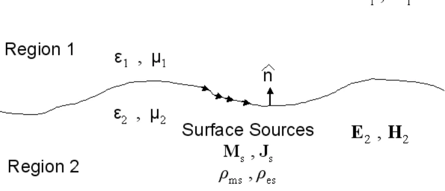
E(r) = − Z dr0∇g(r, r0) × M(r0) −jωµ ·Z dr0g(r, r0)J(r0) + 1 k2∇ Z dr0g(r, r0)∇0· J(r0) ¸ (2.32) H(r) = Z dr0∇g(r, r0) × J(r0) −jω² ·Z dr0g(r, r0)M(r0) + 1 k2∇ Z dr0g(r, r0)∇0· M(r0) ¸ . (2.33) On the other hand, the boundary conditions separating two media of µ1, ²1 and µ2, ²2 (refer to Figure 2.1) where also surface electric and magnetic sources exist are as follows:
ˆ n × E1− ˆn × E2 = −Ms (2.34) ˆ n × H1− ˆn × H2 = Js (2.35) ˆ n · ²1E1− ˆn · ²2E2 = ρes (2.36) ˆ n · µ1H1− ˆn · µ2H2 = ρms. (2.37)
Figure 2.1: Two media with µ1, ²1 and µ2, ²2 where both electric and magnetic current sources exist.
2.1.2
Physical Problem
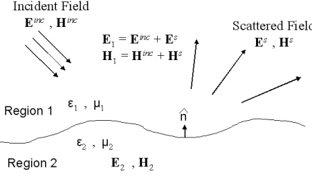
Consider an arbitrarily polarized incident wave (with electric field Einc and mag-netic field Hinc) which illuminates a dielectric surface as depicted in Figure 2.2. Let ²1, µ1 be the permittivity and permeability of region 1 (which is above the interface), respectively, and ²2, µ2 be the permittivity and permeability of region 2 (which is below the interface), respectively. The unit normal ˆn is defined point-ing toward region 1 as shown in Figure 2.2. In region 1, the electromagnetic fields are given by
E1 = Einc+ Es (2.38)
H1 = Hinc+ Hs (2.39)
where Es and Hs are the scattered electric and magnetic fields, respectively. On
the other hand, in region 2, the electromagnetic fields are E2 and H2. Finally, for this situation, the boundary conditions are modified to be
ˆ n × E1− ˆn × E2 = 0 (2.40) ˆ n × H1− ˆn × H2 = 0 (2.41) ˆ n · ²1E1 − ˆn · ²2E2 = 0 (2.42) ˆ n · µ1H1− ˆn · µ2H2 = 0, (2.43)
Figure 2.2: Physical problem describing the scattering from rough dielectric sur-face
since there is neither surface currents nor surface charges at the interface between the regions 1 and 2.
Two equivalent problems, one for region 1 and another for region 2 can be derived and then combined to obtain the resultant integral equations to be used in determining the surface E and H fields.
2.1.3
Equivalent Problem for Region 1
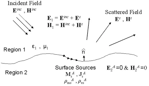
For Region 1 (let’s consider as equivalent problem A), assume the same incident field Einc and magnetic field Hinc and the same electric field E
1 and magnetic field H1 in region 1 as in the physical problem. In this equivalent problem A, let there be equivalent sources on the boundary as seen in Figure 2.3, which satisfy
−MAs = ˆn × E1 (2.44) JA s = ˆn × H1 (2.45) ρA es = ˆn · ²1E1 (2.46) ρAms = ˆn · µ1H1. (2.47)
Figure 2.3: Equivalent problem A for scattering from dielectric rough surface On the other hand, from the boundary conditions given by (2.34)-(2.37), we have
ˆ n × E1− ˆn × EA2 = MAs (2.48) ˆ n × H1 − ˆn × HA2 = JAs (2.49) ˆ n · ²1E1− ˆn · ²2EA2 = ρAes (2.50) ˆ n · µ1H1− ˆn · µ2HA2 = ρAms. (2.51)
Using (2.44)-(2.47) in (2.48)-(2.51), we have EA2 = 0 ,and HA2 = 0 at the boundary. By Huygen’s principle
EA
2 = 0 (2.52)
HA2 = 0 (2.53)
everywhere in region 2 ([30], [31]). Whereas, in region 1 the scattered field gener-ated by these equivalent sources can be derived by considering (2.32) and (2.33):
Es(r) = −jωµ 1 ·Z dS0g 1(r, r0)JAs(r0) + 1 k2 1 ∇ Z dS0g 1(r, r0)∇0s· JAs(r0) ¸ − Z dS0∇g 1(r, r0) × MAs(r0) (2.54)
Hs(r) = −jω² 1 ·Z dS0g 1(r, r0)MAs(r0) + 1 k2 1 ∇ Z dS0g 1(r, r0)∇0s· MAs(r0) ¸ + Z dS0∇g 1(r, r0) × JAs(r0) (2.55) where g1(r, r0) = e −jk1|r−r0| 4π|r − r0|. (2.56)
It should be mentioned at this point that the equivalent sources radiate to whole space. As these equivalent sources radiate into region 2, these fields will cancel the incident fields to yield EA2 = 0 and HA2 = 0 ((2.52) and (2.53)). Note that region 2 also has ²1 and µ1 as region 1. For r in region 2, we thus have the total electric field equation from the extinction theorem as Einc+ Es = 0 yielding
an expression for the incident electric field Einc(r) as
Einc(r) = jωµ1 ·Z dS0g1(r, r0)JAs(r0) + 1 k2 1 ∇ Z dS0g1(r, r0)∇0s· JAs(r0) ¸ + Z dS0∇g 1(r, r0) × MAs(r0). (2.57)
In a similar fashion, from Hinc+ Hs = 0 an expression for the incident magnetic field Hinc(r) can be obtained as
Hinc(r) = jω² 1 ·Z dS0g 1(r, r0)MAs(r0) + 1 k2 1 ∇ Z dS0g 1(r, r0)∇0s· MAs(r0) ¸ − Z dS0∇g1(r, r0) × JAs(r0). (2.58)
Details of the application of Huygen’s Principle and extinction theorem on di-electric rough surface scattering problems can be found in [30] (Section 2.2) or in [31] (Chapter 6).
If we consider (2.57) and (2.58), (2.57) and (2.58) yield overall 6 scalar inte-gral equations, in which the incident fields are known and the equivalent surface current currents are unknown. However, the surface fields (i.e. the equivalent surface currents) cannot be calculated by using them, since they are not inde-pendent. Surface fields (i.e. the equivalent surface currents) further depend on the second medium and its parameters, but µ2, ²2 and g2 (Green’s function for region 2) are not involved in the equations. Thus, we need to solve the equivalent problem for region 2 to conclude the solution to the problem.
2.1.4
Equivalent Problem for Region 2
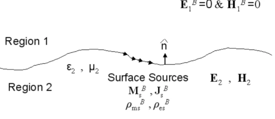
Figure 2.4: Equivalent problem B for region 2 for scattering from dielectric rough surface
Now, let’s consider the equivalent problem B for region 2 with the same electric field E2 and magnetic field H2 in region 2 as in the physical problem. At the boundary we introduce equivalent sources (Figure 2.4), which satisfy
−MBs = ˆni× E2 (2.59) JB s = ˆni× H2 (2.60) ρB es = ˆni· ²2E2 (2.61) ρBms = ˆni· µ2H2 (2.62)
where ˆni = −ˆn. Then similar to the equivalent problem A case, via the help of
boundary conditions given by (2.34)-(2.37), we obtain EB
1 = 0 (2.63)
HB1 = 0 (2.64)
everywhere in region 1. Whereas in region 2, the fields generated by these equiv-alent sources can be obtained by using (2.32) and (2.33) as
EB(r) = −jωµ 2 ·Z dS0g 2(r, r0)JBs(r0) + 1 k2 2 ∇ Z dS0g 2(r, r0)∇0s· JBs(r0) ¸ − Z dS0∇g 2(r, r0) × MBs(r0) (2.65)
HB(r) = −jω² 2 ·Z dS0g 2(r, r0)MBs(r0) + 1 k2 2 ∇ Z dS0g 2(r, r0)∇0s· MBs(r0) ¸ + Z dS0∇g 2(r, r0) × JBs(r0) (2.66) where g2(r, r0) = e−jk2|r−r0| 4π|r − r0|. (2.67)
Similar to the equivalent problem A case, these equivalent sources radiate with the Green’s function g2 to whole space. As these equivalent sources radiate into region 1, these fields will yield EB1 = 0 and HB1 = 0 ((2.63) and (2.64)). Note that we also have ²2 and µ2 for region 1 as well. Thus, for r in region 1, we have the electric field equation which is obtained from EB
1 = 0 as − jωµ2 ·Z dS0g 2(r, r0)JBs(r0) + 1 k2 2 ∇ Z dS0g 2(r, r0)∇0s· JBs(r0) ¸ − Z dS0∇g2(r, r0) × MBs(r0) = 0. (2.68)
In a similar fashion from HB
1 = 0, we obtain − jω²2 ·Z dS0g 2(r, r0)MBs(r0) + 1 k2 2 ∇ Z dS0g 2(r, r0)∇0s· MBs(r0) ¸ + Z dS0∇g 2(r, r0) × JBs(r0) = 0. (2.69)
Since the right hand side of (2.68) and (2.69) are zero (they are not unknowns), then making use of (2.68) and (2.69) results in a total number of 6 scalar integral equations to be solved. However, the surface fields cannot be calculated by using these equations, since they are not independent. This is obvious, because µ1, ²1 and g1 (Green’s function for region 1) are not involved in these equations. Neither is the incident field involved in the above equations. Thus, we also need the equivalent problem for region 1.
Finally, because of the continuity of tangential E and H, and the continuity of normal D and B for the physical problem, and ˆni = −ˆn, we have the following
relations for the equivalent sources A and B. MAs = −MBs (2.70) JA s = −JBs (2.71) ρAes = −ρBes (2.72) ρA ms = −ρBms. (2.73)
2.1.5
Surface Integral Equations for Equivalent Surface
Currents
Surface integral equations are obtained by considering both of the regions and letting both r and r0 be on the interface of region 1 and region 2. Different
surface integral equations can be obtained by taking various combinations of the equations for region 1 and region 2. In this thesis, we considered (2.57) and (2.58) for region 1 (electric field equation and magnetic field equation, respectively), and (2.68) and (2.69) for region 2 (electric field equation and magnetic field equation, respectively).
First let’s start with the cross product of (2.57) and (2.58) with ˆn at the interface. In that case, when r = r0 we will have a singularity to be handled.
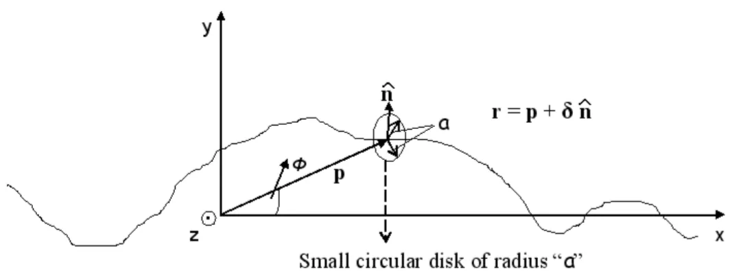
To remove that singularity, the surface S in (2.57) and (2.58) is divided into two regions, namely Sa and P . Sais the area of a circular disk of small radius a about
r and P is the rest of the surface S − Sa. Note that, since we are dealing with a
two dimensional problem in this study, for simplicity, we consider a circular disk rather than a circular sphere. Then, the surface integrals are written as
Z S dS0 = Z Sa dS0+ Z S−Sa dS0 = Z Sa dS0+ Z P dS0 (2.74)
where RPdS0 is known as the principle value (PV) integral. It should be first
mentioned that the first and second integrals of (2.57) and (2.58) are less singular. Therefore, the contributions RS
adS
0 from them will vanish. However, the part
R
SadS
0∇g
1(r, r0) in the third integrals of (2.57) and (2.58) contains a higher order singularity. Because of this, the following procedure is proceeded by regarding
Figure 2.5: A small circular disk of radius a about r.
to the Figure 2.5. Let r = p + δˆn where p is a point on the rough surface and δ is a small scalar quantity. Its sign is more important for us in the following derivations. If δ > 0, then r is infinitesimally above the surface, if δ < 0, then r is infinitesimally below the surface, where ˆn is the normal to the surface at point p. By letting (ρ0,φ0) be the polar coordinates of r0 of circular disk of radius a
centered about p Z Sa dS0∇g 1(r, r0) = Z a 0 dρ0ρ0 Z 2π 0 dφ0∇ 1 4π|r − r0| = Z a 0 dρ0ρ0 Z 2π 0 dφ0 · − (r − r0) 4π|r − r0|3 ¸ = Z a 0 dρ0ρ0 Z 2π 0 dφ0 · −nδ − (ρˆ 0cos φ0x + ρˆ 0sin φ0y)ˆ 4π(ρ02+ δ2)3/2 ¸
The ˆx and ˆy components integrate to zero because of their sin φ0 and cos φ0
coef-ficients, respectively. Thus Z Sa dS0∇g 1(r, r0) = −ˆn δ 2 Z a 0 dρ0ρ0 1 (ρ02+ δ2)3/2 = −ˆn1 2 · − δ (ρ02+ δ2)1/2 ¸a 0 = −nˆ 2 · − δ (a2+ δ2)1/2 ± 1 ¸
where the + sign is for δ > 0 and − sign is for δ < 0. Hence, Z Sa dS0∇g 1(r, r0) = ( −ˆn 2 for δ > 0 ˆ n 2 for δ < 0. (2.75)
Therefore, the third integrals of (2.57) and (2.58) become ˆ n × Z Sa dS0∇g 1(r, r0) × J(r0) = ˆn × µ ˆ n 2 × Js(r) ¶ = −Js 2 = − ˆ n × H 2 (2.76) ˆ n × Z Sa dS0∇g1(r, r0) × M(r0) = ˆn × µ ˆ n 2 × Ms(r) ¶ = −Ms 2 = ˆ n × E 2 . (2.77)
After rearranging the terms, we get the governing surface electric field integral equation and the surface magnetic field integral equation, respectively, for region 1 as ˆ n × Einc(r) = ˆn × Z P dS0∇g 1(r, r0) × Ms− Ms 2 +ˆn × ·Z P dS0jωµ 1g1(r, r0)Js− Z P dS0∇g 1(r, r0) [∇0 s· Js(r0)] jω²1 ¸ (2.78) ˆ n × Hinc(r) = −ˆn × Z P dS0∇g 1(r, r0) × Js(r0) + Js 2 +ˆn × ·Z P dS0jω²1g1(r, r0)Ms− Z P dS0∇g1(r, r0)[∇ 0 s· Ms(r0)] jωµ1 ¸ . (2.79) Following the same procedure for (2.68) and (2.69), the surface magnetic and electric field integral equations, respectively, for region 2 are found as
0 = −ˆn × Z P dS0∇g 2(r, r0) × Ms− Ms 2 −ˆn × ·Z P dS0jωµ 2g2(r, r0)Js− Z P dS0∇g 2(r, r0) [∇0 s· Js(r0)] jω²2 ¸ (2.80) 0 = ˆn × Z P dS0∇g 2(r, r0) × Js(r0) + Js 2 −ˆn × ·Z P dS0jω² 2g2(r, r0)Ms− Z P dS0∇g 2(r, r0) [∇0 s· Ms(r0)] jωµ2 ¸ . (2.81)
Equations (2.78)-(2.81) are the basic integral equations for the electromagnetic scattering problems from dielectric surfaces. Details of the solution for those equations are discussed at Chapter 3.
2.2
Random Rough Surface Generation
In this section, random rough surface generation methodology that is used in this thesis is discussed [29]. Gaussian rough surfaces with Gaussian and Exponential correlation functions are generated.
A one-dimensional random rough surface can be represented by z = f (x), where f (x) is a real valued random rough height function (later we call it as a process) of x with zero mean
Z L
0
xf (x)dx = hf (x)i = 0, (2.82)
where L is the length of the random rough profile.
The Fourier transform of the rough surface height function, f (x), is F (kx) = 1 2π Z ∞ −∞ dxe−jkxxf (x). (2.83)
Then similar to the space domain, in the spectral domain we have
hF (kx)i = 0. (2.84)
The process f (x) is called Gaussian if the random variables f (x1), f (x2), · · · , f (xn)
are jointly Gaussian for any n, x1, x2, · · · , xn [32]. The Gaussian process is
completely characterized by its correlation function hf (x1)f (x2)i = h2C(x1, x2), where h is the root mean square (rms) height.
A rough surface is modelled by a stationary random process, since it is desired to have the surface roughness to be shift invariant, i.e., it should have uniformity. For a stationary random process we have
The Fourier transform of (2.85) is given by h2C(x 1− x2) = Z ∞ −∞ dk1x Z ∞ −∞ dk2xejk1xx1−jk2xx2hF (k1x)F∗(k2x)i. (2.86) Since the left hand side of (2.86) depends only on x1− x2 and f (x) is real (i.e., F∗(k
x) = F (−kx)) then
hF (k1x)F∗(k2x)i = hF (k1x)F (−k2x)i = δ(k1x − k2x)W (k1x) (2.87)
where W (kx) is known as the spectral density. The Fourier transform of h2C(x)
is the spectral density W (kx) given by [32]
h2C(x) =
Z ∞
−∞
dkxejkxxW (kx). (2.88)
The right hand side of (2.87) is nonzero only if k1x = k2x, so F (k1x) and F∗(k2x) are independent random variables, then (2.87) equals to zero,
hF (k1x)F∗(k2x)i = hF (k1x)ihF∗(k2x)i = 0. (2.89)
Now, let’s consider that f (x) is a periodic function with periodicity of L, i.e., f (x) = f (x + L). We can represent f (x) via its Fourier series as
f (x) = 1 L ∞ X n=−∞ bne j2πnx L (2.90)
where bn is Gaussian distributed which will be shown shortly. From (2.85) and
(2.90) we have hf (x1)f (x2)i = 1 L2 ∞ X n=−∞ ∞ X m=−∞ hbnb∗mie j2πnx1 L e−j2πmx2L . (2.91) By using (2.85) and (2.87) in (2.86) hf (x1)f (x2)i = h2C(x1− x2) = Z ∞ −∞ dkxejkx(x1−x2)W (kx), (2.92) and by equating (2.91) to (2.92) Z ∞ −∞ dkxejkx(x1−x2)W (kx) = 1 L2 ∞ X n=−∞ ∞ X m=−∞ hbnb∗mi exp µ j2πn L (x1− x2) ¶ , (2.93)
(2.93) can be written as 2π L ∞ X n=−∞ ejKn(x1−x2)W (K n) = 1 L2 ∞ X n=−∞ ∞ X m=−∞ hbnb∗miejKn(x1−x2) (2.94) where Kn = 2πn L = n∆kx. (2.95) From (2.94), hbnb∗mi = 2πLW (Kn). (2.96)
Since bn and bm are independent, hbnb∗mi is zero unless m = n. Thus,
h|bn|2i = 2πLW (Kn). (2.97)
When f (x) is real, Fourier series coefficients satisfy,
bn = b∗−n. (2.98)
Then from (2.96), we know that
hbnb∗−ni = 0. (2.99)
Combining (2.98) and (2.99) results in
hbnbni = 0. (2.100)
If we represent real and imaginary parts of bn as <(bn) and =(bn), respectively,
bn= <(bn) + j=(bn), (2.101)
(2.100) results in
h(<(bn))2i = h(=(bn))2i (2.102)
h<(bn)ih=(bn)i = 0. (2.103)
Thus <(bn) and =(bn) are independent Gaussian random variables, N (0,h|bn|
2i
2 )
(with mean zero and variance equal to half of that of h|bn|2i), so bnturns out to be
Gaussian surface can be represented by a Fourier series with Gaussian distributed coefficients satisfying (2.98)-(2.102).
In order to generate N independent Gaussian random numbers, which are Fourier series coefficients for Gaussian surface formulation, we divide the surface L into N units and we use a DFT (discrete Fourier transform) version of (2.90). Let there be N points in both space and spectral domains, then the unit distance will be ∆x = L N (2.104) and xm = m∆x (2.105) for m = −N 2 + 1, · · · , 0, 1, · · · , N 2 (2.106) f (xm) ≡ fm. (2.107) Then fm = 1 L N 2 X n=−N 2+1 bnexp µ j2πnm N ¶ . (2.108) The DFT is bn = L N N 2 X m=−N 2+1 fme−j 2πnm N . (2.109)
Equations (2.108) and (2.109) can readily be computed by FFT. Both fm and bn
are periodic with period N. That is,
bn+N = bn (2.110)
fm+N = fm. (2.111)
Hence,
b−N
2 = bN2. (2.112)
Moreover from (2.98) we know that b−N
2 = bN2 = b
∗
Then (2.112) and (2.113) yield both b+N
2 and b0 are real.
We have shown that any periodic discrete function has special DFT coeffi-cients satisfying (2.110)-(2.113). Using MATLAB, we can generate independent Gaussian random numbers satisfying these special conditions, thus a random Gaussian surface using inverse DFT. Below is the MATLAB methodology given in step by step format:
1. With a given seed, N Gaussian distributed random numbers that have zero mean and unit variance are generated using MATLAB function randn. These N numbers are independent and they are not required to be grouped or arranged in any order. Let the numbers be labeled as r1, r2, · · · , rN.
2. Then two real Gaussian numbers b+N
2 and b0 are calculated as
b0 = p 2πLW (0)rα (2.114) b+N 2 = r 2πLW (πN L )rβ (2.115) where α 6= β and α, β ∈©1, 2, · · · , Nª.
3. (N/2 − 1) Gaussian numbers are calculated by using bn= p 2πLW (|KN|) · 1 √ 2(rσ + jrξ) ¸ (2.116) for n = −N
2 + 1, · · · , −2, −1 where σ, ξ are distinct indices selected from set S =n©1, 2, · · · , Nª/©α, βªo.
4. Using (2.98),
bn= b∗−n (2.117)
bn for n = 1, 2, · · · ,N2 − 1 can be calculated in a straightforward way.
5. Finally, using the inverse DFT relation in (2.118) with X(n) = bn,
x(m) = 1 N N 2 X n=−N 2+1 X(n)e2πjN mn (2.118)
x(m), m ∈ ©1, 2, · · · , N − 1ª is obtained. Extending x(m) periodically, rough surface height profile is figured out as
fm = N
Lx(m) (2.119)
for m = −N
2 + 1, · · · ,N2.
Our method in this study is to evaluate the derivative and higher order deriv-atives of the rough surface profile by means of finite difference
f0(x m) =
f (xm+ 1) − f (xm− 1)
2∆x . (2.120)
For the two endpoints m = −N
2 + 1 and m = N2, we use the periodic condition of DFT to get f (xm) for m = −N2 and m = N2 + 1.
2.2.1
Gaussian Spectrum
For the case that the correlation function is Gaussian C(x) = exp µ −x 2 l2 ¶ . (2.121)
Using (2.88), the Gaussian Spectral Density can be shown to be W (kx) = h 2l 2√πexp µ −k 2 xl2 4 ¶ (2.122) where h is rms height, l is correlation length, and kx is surface wavenumber. It
also holds that,
l =√2h
s (2.123)
where s is the rms slope.
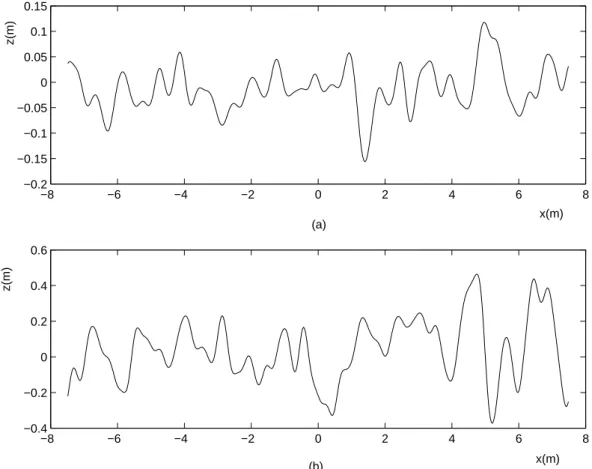
In Figure 2.6a, there is a Gaussian correlated moderately rough profile that has rms height of λ/6 and correlation length of λ, so the rms slope is approximately 13◦. In Figure 2.6b, there is a Gaussian correlated very rough profile that has rms
height of 0.707λ and correlation length of λ, so the rms slope is approximately 45◦. The frequency is set to 1 GHz for both of the cases (λ = 0.3m).
−8 −6 −4 −2 0 2 4 6 8 −0.4 −0.2 0 0.2 0.4 0.6 x(m) z(m) −8 −6 −4 −2 0 2 4 6 8 −0.2 −0.15 −0.1 −0.05 0 0.05 0.1 0.15 x(m) z(m) (a) (b)
Figure 2.6: (a)Gaussian correlated moderately rough surface with σ = λ/6, Lc =
λ, so that the rms slope is = 13◦ at 1 GHz (b)Gaussian correlated very rough
surface with σ = 0.707λ, Lc= λ, so that the rms slope is = 45◦ at 1 GHz
2.2.2
Exponential Spectrum
Similarly, when the correlation function is exponential, i.e., C(x) = exp µ −|x| l ¶ , (2.124)
the Exponential Spectral Density can be shown to be W (kx) = h2l π 1 1 + k2 xl2 (2.125) where h is rms height, l is correlation length, and kx is surface wavenumber.
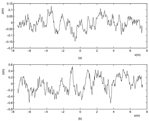
that has rms height of λ/6 and correlation length of λ, so the rms slope is ap-proximately 13◦. In Figure 2.7b, there is an exponentially correlated very rough
profile that has rms height of 0.707λ and correlation length of λ, so the rms slope is approximately 45◦. The frequency is set to 1 GHz for both of the cases
(λ = 0.3m). −8 −6 −4 −2 0 2 4 6 8 −0.8 −0.6 −0.4 −0.2 0 0.2 0.4 0.6 x(m) z(m) −8 −6 −4 −2 0 2 4 6 8 −0.2 −0.15 −0.1 −0.05 0 0.05 0.1 0.15 x(m) z(m) (a) (b)
Figure 2.7: (a)Exponentially correlated moderately rough surface with σ = λ/6, Lc = λ, so that the rms slope is = 13◦ at 1 GHz (b)Exponentially
corre-lated very rough surface with σ = 0.707λ, Lc= λ, so that the rms slope is = 45◦
2.3
Method of Moments
The method of moments (MoM) is a numerical technique that has been widely used to evaluate the field scattered by (deterministic) metallic objects in antenna and radar applications. Many detailed and interesting texts have been written on MoM [28],[33]. However, its use in the evaluation of scattering from random rough dielectric surfaces is not so widespread and is more recent. In fact, it has been first presented in [5]. In this section, we recall main concepts of the method. MoM converts an equation that contains a linear operator into a matrix equa-tion, which can be solved by matrix inversion. Often, the operator is an integral, which just as often contains an integrand with a singularity.
With the use of Green’s function, integral equations can be derived that we have discussed at the beginning of this chapter. Consider a one dimensional integral equation of the form
Z b
a
dx0G(x, x0)f (x0) = c(x) (2.126)
where G(x, x0) is the Green’s function, f (x0) is the unknown for the domain
a ≤ x0 ≤ b, and c(x) is known for a ≤ x ≤ b. To solve (2.126), two sets of
functions are used in the MoM: Basis functions and weighting functions.
1. Basis functions: In the domain of a ≤ x ≤ b, a set of N basis functions are chosen and they are labelled as f1, f2, ..., fN. Then the unknown function
f (x0) is written in terms of linear combinations of these basis functions as
f (x0) = N
X
n=1
bnfn(x0). (2.127)
The number of basis functions has to be chosen well in a sense that the linear combination of fn(x0) should well represent the unknown f (x0) in the
domain. Next, the equation (2.127) is substituted into (2.126) to obtain
N X n=1 bn Z b a dx0G(x, x0)f n(x0) = c(x). (2.128)
If the unknown coefficients b1, b2, ..., bn are determined then the solution is
achieved.
2. Now one equation with N unknowns is obtained. However, N indepen-dent equations with the same unknowns have to be derived in order to find a solution. Next a set of N weighting functions (testing functions) w1(x), w2(x), ..., wN(x) is chosen. Multiplying (2.128) by wm(x) and
inte-grating the result over the domain yields
N X n=1 bn Z b a dxwm(x) Z b a dx0G(x, x0)fn(x0) = Z b a dxwm(x)c(x). (2.129)
(2.129) gives the matrix equation
N X n=1 Gmnbn = cm (2.130) with m = 1, 2, ..., N , and cm = Z b a dxwm(x)c(x) = hwm, ci (2.131) Gmn = Z b a dxwm(x) Z b a dx0G(x, x0)fn(x0) = hwm, Gfni (2.132)
where the inner product notation is used such that hf, gi =
Z b
a
dxf (x)g(x). (2.133)
2.3.1
Computational Considerations
For the matrix equation (2.130) the following notes have to be taken into account. • Matrix solution: To solve a full matrix equation of order N by matrix inversion (e.g., LU decomposition or Gaussian elimination), O(N3) number of operations will be required. Because of this, the number of operations, and so the solution time rapidly increase with an increase in N
• The unknown function: The unknown function f (x) has to be decomposed into a suitable number of pieces, fn(x), in order to well represent the correct
solution.The number of fn, n = 1, 2, ..., N should be neither so high that the
computational cost increases nor so low that the accurate solution cannot be achieved.
2.3.2
Basis Functions
Either entire domain or subsectional basis functions can be used. Entire domain basis functions are nonzero over the entire domain of the structure (a, b) such as sines, cosines, etc. On the other hand, subsectional basis functions are nonzero over a small (subsectional) part of the entire domain such as pulse, rooftop, piecewise-sinusoidal basis functions.
A common choice for rough surface scattering type problems is the pulse basis function, which is a subsectional basis function in the form of
fn(x) =
(
1 if an≤ x ≤ bn
0 otherwise (2.134)
where the interval a ≤ x ≤ b has been divided into N intervals with endpoints an and bn, for n = 1, 2, ..., N.
2.3.3
Weighting Functions
There are two common choices for the weighting functions.
1. Galerkin’s Method: In this case, the weighting functions are the same as the basis functions, i.e., wn(x) = fn(x).
2. Point Matching Method: One can pick a set of points x = x1, x2, ..., xN to
enforce (2.128). Then N X n=1 bn Z b a dx0G(x m, x0)fn(x0) = c(xm) (2.135)
where cm = c(xm) (2.136) Gmn = Z b a dx0G(x m, x0)fn(x0). (2.137)
This particular choice of testing procedure is called point matching. In terms of weighting functions, this means that the weighting functions are
wm(x) = δ(x − xm) (2.138)
where m = 1, 2, ..., N and δ is the Dirac delta function.
In this thesis, MoM solutions are used as the reference solution. The basis functions are chosen as pulse functions and the weighting functions are chosen as Dirac delta functions.
In this chapter, the necessary background information and the governing sur-face integral equations for the scattering of electromagnetic waves from random rough dielectric surfaces are introduced. The solution methodology to this prob-lem and the improvements are discussed next.
Solution for the Problem
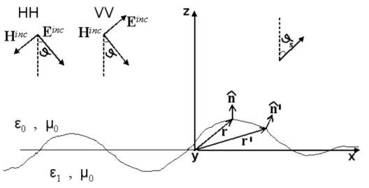
Figure 3.1: Geometry of scattering from dielectric random rough surface problem As we discussed in Chapter 2, the solution to the problem of scattering of electromagnetic waves from random rough surfaces starts with the derivation of the corresponding surface integral equations. Then, MoM will be applied to those integral equations to solve for the unknowns.
Consider the geometry depicted in Figure 3.1. Surface height profile and elec-tromagnetic fields are assumed to be constant along the y-direction. ”HH” means that both the incident and scattered electric fields are horizontally polarized (i.e.
they have only ˆy component) and ”VV” means both the incident and scattered electric fields are vertically polarized (i.e. they don’t have any ˆy component). For this geometry, if the incident field is horizontally polarized, then the surface electric and magnetic fields can be evaluated solving the following pair of integral equations derived in Chapter 2 given by (2.78) and (2.80)
ˆ n × Einc(r) = −Ms(r) 2 + ˆn × Z S · jωµ0φ0(r, r0)Js(r0) − Ms(r0) × ∇φ0(r, r0) −∇ 0 s· Js(r0) jω²0 ∇φ0(r, r0) ¸ ds0 (3.1) 0 = −Ms(r) 2 − ˆn × Z S · jωµ0φ1(r, r0)Js(r0) − Ms(r0) × ∇φ1(r, r0) −∇ 0 s· Js(r0) jω²1 ∇φ1(r, r0) ¸ ds0. (3.2)
On the other hand, if the incident field is vertically polarized, then the surface electric and magnetic fields can be evaluated by solving the following pair of integral equations derived in Chapter 2 given by (2.79) and (2.81)
ˆ n × Hinc(r) = Js(r) 2 + ˆn × Z S · jω²0φ0(r, r0)Ms(r0) + Js(r0) × ∇φ0(r, r0) −∇0s· Ms(r0) jωµ0 ∇φ0(r, r 0) ¸ ds0 (3.3) 0 = Js(r) 2 − ˆn × Z S · jω²1φ1(r, r0)Ms(r0) + Js(r0) × ∇φ1(r, r0) −∇0s· Ms(r0) jω²1 ∇φ1(r, r 0) ¸ ds0 (3.4)
where ˆn is the unit outward normal to the surface. In (3.1)-(3.4), Ms= −ˆn × E
is the equivalent surface magnetic current density, Js = ˆn × H is the equivalent
surface electric current density and both r and r0 belong to the surface profile.
First terms in (3.1)-(3.4) correspond to the case where r = r0. Since we are
dealing with a two-dimensional problem, the integrals Rsds0 become R
ldl0 and
we use the two dimensional free-space Green’s function which is the zeroth order Hankel function of the second kind given by
φ0,1(r, r0) = − j 4H
(2)
0 (k0,1|r − r0|) (3.5)
where k0, k1 are the propagation constants of the upper and lower media, re-spectively. Equations (3.1)-(3.4) assume the lower space to be homogeneous, unlimited, and with the same magnetic permeability, i.e. µ0, of the upper one.
3.1
HH Polarization
For the scattering geometry given in Figure 3.1, the horizontally polarized incident fields are
Einc = ˆyejk0(−x sin ϑ+z cos ϑ) (3.6)
Hinc = 1
η(−ˆx cos ϑ − ˆz sin ϑ)e
jk0(−x sin ϑ+z cos ϑ) (3.7)
where η is the free-space intrinsic impedance. Also the induced electric surface current density on the surface is only a function of the surface contour variable r0, therefore
∇0
s· Js= 0. (3.8)
This leads to a simplification to the pair of electric surface field integral equations, (3.1) and (3.2), resulting ˆ n × Einc(r) = −Ms(r) 2 + ˆn × Z l · jωµ0φ0(r, r0)Js(r0) − Ms(r0) × ∇φ0(r, r0) ¸ dl0 (3.9) 0 = −Ms(r) 2 − ˆn × Z l · jωµ0φ1(r, r0)Js(r0) − Ms(r0) × ∇φ1(r, r0) ¸ dl0 (3.10) where l is the surface profile.
By using the following vector identity
Ms× ∇φ0,1 = (−ˆn0× E) × ∇φ0,1= −E(ˆn0· ∇φ0,1) (3.11)
and considering only the scalar form of the equations, (3.9) and (3.10) can be further simplified to Einc(r) = E(r) 2 + Z l ½ jωµ0φ0(r, r0)Js(r0) + E(r0) £ ˆ n0· ∇φ 0(r, r0) ¤¾ dl0 (3.12) 0 = E(r) 2 − Z l ½ jωµ0φ1(r, r0)Js(r0) + E(r0) £ ˆ n0· ∇φ1(r, r0) ¤¾ dl0 (3.13) where Einc = Eincy and E = E ˆˆ y are incident and total electric fields, respectively.
Using rectangular pulse basis functions and the point matching method, the integral equation pair (3.12)-(3.13) can be converted into a pair of matrix equa-tions for the unknowns E and Js given by
S0E + Z0Js = Einc
S1E + Z1Js = 0 (3.14)
where · stands for a matrix and · stands for a vector. Equation (3.14) can be expressed in a more compact from as
A x = y (3.15) with Amn= Ã S0mn Z0mn S1mn Z1mn ! , xn= Ã En Js,n ! , ym = Ã Einc m 0 ! (3.16) where the size of the matrix is 2N × 2N, with N being the number of rectangular pulse basis functions used to expand the unknown current density Jy and the
unknown surface field Ey over the entire illuminated surface contour. The full
expressions for the coefficients of the matrix elements can be obtained as S0mn = 1 2δmn+ Z ∆ln ˆ n0· ∇φ 0dl0 ∼ = 1 2 − (d2z/dx2) n∆x 4π[1+(dz/dx)2 n], m = n jk0 4 (ˆnn· R)H (2) 1 (k0|rm− rn|) p 1 + (dz/dx)2 n∆x, m 6= n (3.17) Z0mn = jωµ0 Z ∆ln φ0dl0 ∼ = jωµ0 −j 4 µ 1 − 2j πln γk0 √ 1+(dz/dx)2 n∆x 4e ¶ p 1 + (dz/dx)2 n∆x, m = n −j4H0(2)(k0|rm− rn|) p 1 + (dz/dx)2 n∆x, m 6= n (3.18) S1mn = 1 2δmn− Z ∆ln ˆ n0 · ∇φ 1dl0 ∼ = 1 2 + (d2z/dx2)n∆x 4π[1+(dz/dx)2 n], m = n −jk1 4 (ˆnn· R)H (2) 1 (k1|rm− rn|) p 1 + (dz/dx)2 n∆x, m 6= n (3.19)