Computation of optimal H∞ controllers and Approximations of fractional order systems: A tutorial review

Appl. Comput. Math., V.12, N.3, 2013, pp.261-288

COMPUTATION OF OPTIMAL

rf.

00

CONTROLLERS AND

APPROXIMATIONS OF FRACTIONAL ORDER SYSTEMS:

A TUTORIAL REVIEW

.. 1 • 1 .. 1

A.E. KARAGUL, 0. DEMIR, H. OZBAY

ABSTRACT. This paper briefly reviews the recent techniques in the field of fractional order systems, and concentrates on the design of 'H00 optimal controllers for a magnetic suspension system model, derived in (25). The plant involves infinite dimensional terms, including a time delay and a rational function of y's. The recent formulation in (36) is used for the controller design, solving the mixed sensitivity minimization problem for unstable infinite dimensional plants with low order weights, and the result is verified with the old design procedure of (44). For simulation purposes, various implementation methods are performed, and a new approximation method is proposed.

Keywords: Fractional Order Systems, 'H00 Optimal Control, Approximation of Fractional Order Systems, Time Domain Simulations of Fractional Order Systems.

AMS Subject Classification: 26A33, 93C80, 49J99.

1. INTRODUCTION

"Can the meaning of derivatives with integer order be generalized to derivatives with non-integer orders?" This question was raised by Leibniz in a letter to L'Hopital (31] introducing the fractional order calculus where the orders of integration and differentiation are fractions. To create an insight, an n-fold integral can be considered:

I

rt

rt

f(y)(t - y)n-I

···lo

f ( y ) ~

=

lo

(n-1)!

dy .

...____,. n

n

For the case

n

E

JR+,

the Riemann-Liouville definition for the fractional order integral is obtained

(30]

ft

f(y)(t - y)n-l

1

t

n-1

lo

(n -

1}!

dy

=

r(n)

lo

J(y)(t -

y)

dy.

Generalization of the formula for the

n

times iterated derivation, for the case

n

E

JR+,

gives the Griinwald-Letnikov's definition for the fractional order derivative [41]. Another definition for the fractional order derivative is Caputo's definition [42]:

Q - 1

rt

i/)..+l<y)

D f(t) -

f{l - 8)

lo

(t - y)

6

dy,

where

a

=

d

+

8,

d

E Z, and O

<

8

~ 1.

During the last decades, application of the fractional order calculus to the field of feedback control has attracted many researchers. This manifests itself in the increasing number of papers

1_{Dept. of Electrical and Electronics Engineering, Bilkent University, 06800 Ankara, Turkey}

Corresponding author e-mail: [email protected]

Manusc1-ipt received 9 October 2019.

262 APPL. COMPUT. MATH., V.12, N.3, 2013

on fractional order systems and control. According to Caputo's definition, the Laplace transform of the fractional order integral is [9, 10]

('° ( -

1-

t

J(y)(t -

Yt-

1_{dy) e-stdt}

=

_{s-o: F(s), where a> 0.}

lo

r(a)

lo

A fractional order system can be represented by the transfer function

bmsf3m

+

bm-is13m-l

+ ... +

bosf3o

G(s)

=

,

OnS°'"

+

On-lSOn-l

+ """ +

OQS°'O

where f3k and Oj are rational numbers, for k

=

0, 1, ... , m; and j

=

0, 1, . . . , n. . The same system can also be represented by the following equation in time domain

anD°'"y(t)

+

On-1D0 n-ly(t)

+ · · · +

aoD00_y(t)

=

=

bmDf3mu(t)

+

bm-1D/Jm-1u(t)

+ · · · +

boDf3ou(t),

here D"f f(t) denotes the Caputo derivative of order ,, and Oi,

/3j

for i E {O, 1, ... , n }; j E {O, 1, ... ,m} are rational numbers; and

{ao,a1, ...

,an},

{bo,b1, ... ,bm}

are real constants.

One of the first researchers realizing the importance of the fractional order calculus in control theory is Bode. He has called the following the ideal open loop transfer function [1, 41]

A

F(s)

= -,

(1)

so:

where A

>

0, and a needs to satisfy O

<

a

<

1 for the phase margin to be greater than 1r /2 .

In fact, small values of a result in large values of the phase margin. This is one of the main principles of Bode's loop shaping, which says that at the gain crossover frequency, the magnitude drop should be small to have a large phase margin [15]. This allows the phase margin of the feedback system to be invariant to the changes in the amplifier gain. The transfer function in (1) includes an irrational function of the Laplace variables, so being infinite dimensional, it has unlimited memory.

In the 1990s, [33] proposed a non-integer order robust control method, called CRONE. In [42], superior performance of the fractional order controller PI ADµ over the classical PI D controller is shown. An algorithm for the co-design of gain and phase margins using fractional order PI A

controllers is presented [48]. A set point weight rules for PI ADµ controllers is addressed in [38]. A PIO controller design algorithm for fractional order systems with time delays is presented in [37]. Besides P JADµ and CRONE algorithms, 'H.2 and 'H.00 control strategies are also proposed for

fractional order systems [28, 39]. Variable order fractional controllers are proposed in [46], aiming a constant phase margin. For fractional order systems with time delay, a stabilization algorithm by using PI ADµ controllers is given in [22] . In [8], a fractional order controller is designed for a DC-DC buck converter by using frequency domain techniques. Other applications involve controller designs for a hydraulic actuator [43], flexible transmission [35], a robot manipulator [16], and a lightweight flexible manipulator [32]. For fractional order nonlinear discrete time systems, a switched state model predictive control is provided in [14]. A second order D0 type

iterative learning control scheme for fractional order systems is presented in [26]. For fractional s~~~"!,~~h ~i~e: c!elays, stability windows can be d~ter~ined by using the numerical procedure out~i~vt:~;:t.tl\TLAB toolbox, YALTA, which 1s based on [5, 17, 18, 20] can be used for the stability aiia1ysis of classical and fractional systems with commensurate delays [2]. The bounded input bounded output stability condition for distributed-order systems over the integral interval (0,1), has been established in [24].

It is widely known that there arc physical devices that can perform fractional order integra-tion or differentiaintegra-tion [4]. Approximate implementaintegra-tions can also be performed by frequency domain ~tting techniques in continuous or discrete time. For example, Carlson's method [11], Matsuda s method [29], and Oustaloup's method [34] can be used to obtain continuous rational approximates of fractional order systems. For discrete equivalences, FIR implementation can

A.E . KARAGUL et al. : COMPUTATION OF OPTIMAL 1-f."° CONTROLLERS .. . 263

be performed. For alternative discretization methods, see [13, 45]. Furthermore, MATLAB's invfreqs command can be used for approximations of fractional order transfer functions from the frequency response data. Various methods for analog circuit realizations of fractional order systems can be found in [3, 40].

In this paper, the following standard feedback system depicted in Fig. 1, is considered. d(t)

e(t)

C(s) t---1~+-~---.i

/'(s)

y(t)

Figure 1. Standard feedback system.

A feedback loop involving fractional order systems can be classified in two groups

(i) a fractional order controller used for a finite dimensional plant,

( ii) an integer or fractional order controller used for a fractional order plant.

To our knowledge, most of the existing literature on this subject a.dresses feedback loops of type

( i), in other words, fractional order controllers are designed for rational plants.

As an example, consider a minimum phase plant P(s). By virtue of Bode's loop shaping, choose a fractional order controller so that, open loop system has the following transfer function

C(s) = ;( )'=> G(s) =~.with k

>

0, and

a>

0.

s0 s s0

A closed loop system is stable for k

>

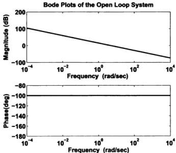
0, and the phase margin can be specified with the proper choice of a. The phase margin of such a system is (1r - (1r /2)o), and crossover frequency is k1_{1°. With a certain set of requirements, a controller can be designed. For example, for} PM= 80°, a is equal to 1.1, and for cut-off frequency (we) of 5 rad/sec, k should be equal to

6, since k = we O • Fig. 2 illustrates the magnitude and phase plots of the Bode's ideal open loop system with k = 6 and a = 1.1. The unit step response is shown in Fig. 3.

The above discussion is valid for minimum phase plants. In case of a non-minimum phase plant, the methods presented in [8] can be followed to compensate the effects of the right half plane zeros.

Bode Plots of the Open Loop System

-so.---~~~~~~~~~~~~~-. ii - 1 0 0 . . - - - i !-120

•

I

-140 ~ a. -160 -1ao~~~~~~~~~~~~~~~ 10-4 10-2 _{10° 10}2 _10• Frequency (rad/sec)

264 APPL. COMPUT. MATH., V.12, N.3, 2013

Step Response of the Closed Loop System

1.4 ~ - ~ - - - - , - - - . - - - ~ - - . 1.2 G) 1 / [ 0.8 Ill G) 0: a. 0.6 G) ui 0.4 0.2 0_{o 2 4 6 8 10} Time In sec.

Figure 3. Step response of the closed loop system with G(s)

=

;h

-The present work deals with a feedback system of type (ii), and concentrates on a specific fractional order plant to illustrate an 1i00 controller design method. Recently, a mathematical model of the non-laminated magnetic suspension system is derived in a series of papers [25 , 49] This work deals with computing the 1i00 optimal controller for the system model derived in [25, 49]. The transfer function of the system is in the form of a rational function of

..js,

followed by a time delay term e - hs, where h

>

0 represents the time delay. The method proposed in [44], can be used to compute the 1i00 _{optimal controller for such infinite dimensional systems.} Later in [36], the method in [44] has been simplified for the case where the sensitivity weight is low-order. In this paper, the mixed sensitivity minimization problem will be solved for the unstable fractional model developed in [25, 49]; using the method in [36], and this will be verified by the old design procedure of [44].

In Section 2, the mathematical model of the plant is described. In Section 3, a detailed discussion on the computation of the 1i00 optimal controller is given. Section 4 outlines some recent techniques for implementation of fractional order terms in the optimal 1i00 controller

expression and outlines a new approximation technique based on frequency-response data. Time d·omain simulation results are given in Section 5. Finally, concluding remarks are made in Section

6.

2. DESCRIPTION OF THE FRACTIONAL ORDER PLANT MODEL CONSIDERED

This section analyzes the fractional order plant model of a non-laminated magnetic suspension system model given by [25]. Actuator and/or sensor time delays (due to real time data acquisition and transmission) may be present resulting in the following transfer function

e-h.s

P(s)

=

.

(s0 )5

+

_(s0 )4 - c (2)

In (2), s is the Laplace variable, h

>

0 is the time delay, and o: is a rational number o: E (0, 1). For this plant, a

=

0.5 is fixed, [25]. For finding the locations of the poles, the following transformation is used

(=So.

With this transformation, the stability region in the (-plane is as follows [19]

IL(I

>

0:7r .

A.E. KARAGUL et al.: COMPUTATION OF OPTIMAL 'H.00 _{CONTROLLERS .. . 265}

In [25], it is shown that for all c

>

0, the plant has only one unstable real pole and 4 complex stable poles. Locations of the poles are computed, as shown in Fig. 4. Taking c

=

5, produces the poles in the ( plane, shown in Table 1.

Locations of the Poles of the Plant in ~ -domain 10.---~~~~~~~~--=~~~~~ 5 0 -5 -10L--~~~~~ ~~~--=~~~~--.3' -10 -5 0 5 10

Figure 4. Locations of the poles of the plant in [25] for 10-5 < _c < _{105 .} Solid line shows the stability region in the (-domain.

Table 1. Locations and the Phases of the Roots of (5 _{+ (4 - 5 = 0.} Locations of the Roots the Phases

Pi

=

-1.3665 + j0.7563 150° P2

=

-1.3665 - j0.7563 -150°

p3

=

0.2542

+

jl.2687 78°

p4

=

0.2542 - jl.2687 -78°

p

=

1.2244

oo

Then, the transfer function of the plant can be re-written as

1 1

P(s) = e-hsG(s0 ) _G(s0 ) =

-(s0 - p), (sa - p1)(sa - P2)(sa - p3)(sa - p4),

where G(s0 ) is the stable and minimum phase part of the system, and Bode plots of G(s0 ) are

given in the Fig. 5.

Bode Plots of the Stable Part of the Plant Model

t:=r =·==•=:sJ===

1~ 1~ 1i 1i 1~

Frequency (rad/sec)

~

:::~1

.

~~~:

I

1~ 1~ 1i 1i 1~

Frequency (rad/sec)

266 APPL. COMPUT. MATH., V.12, N.3, 2013

3. OPTIMAL 'H00 _{CONTROLLER DESIGN}

This section deals with designing the optimal 'H00 _{controller for the plant described in the}

previous section. The plant is infinite dimensional, including irrational terms ,/sand e-hs . The technique proposed in [44] can be used to compute the mixed sensitivity minimizing controllers for such infinite dimensional plants. This method for the case where the sensitivity weight is low-order is simplified in [36]. In this section, these two algorithms will be applied separately to find the optimal 'H00 controller. The section is divided into four subsections. In the fi~st

part, factorization of the plant is given, then in Subsection 3.2 and 3.3, two methods are applied separately to compute the optimal controller. In Subsection 3.4, the controller expression is given.

3.1. Factorization of the Plant. The mixed sensitivity minimization problem tries to find the optimum performance level and the corresponding optimal controller

rapt =

=

crd(P)

II

[w,g(7 :~~/-

1] 11₀₀

=

II

[w2~b~t11:c;~~:)-

1] 11_{00 '}

where C(P) denotes the set of all controllers stabilizing the feedback loop formed by the plant

P and the controller C, and W1 and W2 are rational weighting functions shaping the desired sensitivity and the complementary sensitivity, respectively. Typically, W1 ( s) is a low-order, low pass filter representing a reference signal generator, and W2(s) is a high pass filter, representing an upper bound on the multiplicative plant uncertainty. Recall that a feedback system is stable if and only if (1

+

PC)-1 , P(l

+

PC)-1 _{and C(l}

+

_PC)-1 _{are all in 'H00 •}

The plant. under consideration given by (2), can be factorized as follows

(3)

In (3), No(s) is an outer function, Mn(s) is an inner function, and Md(s) is an inner function whose zeroes 0:1 , . . . , o:, € C+ are the unstable poles of the system. The technique proposed in

[44] requires Md(s) to be a rational function of s. Therefore, to factorize the plant we use the fact t~at a= 0.5 and (s0 - p)(s0

+

p)

=

_{(s -} p_{2 ) .} Hence, the factorization

Mn(s)

=

e-hs, Md(s)

=

(s - p2), and N0(s)

=

(sa

+

p)

(s

+

r)

(s

+

p2)(s0 - P1)(s0 - P2)(s0 - p3)(s0 - p4).

Thus, in the specific example considered here, we have l = l and o:1 = p2 • In this work, for simplicity of exposition low-order weights are chosen

1

W1(s)

= -,

W2(s)

=

ks, where k

=

0.3 s

and the notation W1

=

nWifdW1 is used with nW1(s)

=

1 and dW1(s)

=

s . The choice of

W1 ( s) guarantees zero steady state error for step like reference signals. Note that representation of N0 ( s) is not minimal in s0

3.2. Toker-Ozbay Formula. For the factorized plant, given in (3), the 'H00 controller can be

written in the form below (see [44])

C

=

E₁Afd N-1F1L I +MnF"( L (4) with E ( ·) _ lVi(- s)W1(s) dW1(-s) -, -~ - ₂ - 1, F-,(s )

=

₁G₁(s ). 'Y nWI(s)

A.E. KARAGUL et al. : COMPUTATION OF OPTIMAL ?t00 CONTROLLERS .. . ₂₆₇

where the stable G-y(s) is found from the spectral factorization

G (s)G (-s)

=

(i

+

W2 -s W2 s _ W2(-s~W2(s)

)-l .

'Y 'Y W1 -s W1 s) -y

Then, the controller achieves optimum performance level with ,opt, and L(s) is determined from a set of linear equations as described below. The following equations are performed to find "(opt and L(s) . Define L(s)

( ) _ [ 1 s ... sn-

l]

\JI

2

L s - [ 1) ,

1 S ... Sn- \JI l (5)

where n := n1

+

l, with n1 = deg(dWi). The unknown coefficients \J1 1 and \J12 are defined in the

following way: \J11

=

['¢10 ...

1P1(n-1)f, \J12

=

[w20 ...

1P2(n-1)f. The relationship between \J11 and \J12 is

\JI l =

±.Jn

\J12,

Jn

\J12 =: ~,

where

Jn

is an x n diagonal matrix, whose ith diagonal entry is equal to (-l)i+1. The function

L( s) is determined from ~, the singular vector of R, corresponding to the zero singular value obtained by the largest feasible 1

>

0

R,~=0,

where the parameterized matrix R, is given by

'O [Va1 Va Va ni] [ Vi

O]

[Va1 Va Va ni] .:J, '""Y

=

V,a1 V,a V,an1

±

0 Vn₁ V,a1 V,a V,an1 n·

The above definition uses the following

Vn

=

blockdiag(Vl, Vn1 ).

(6)

(7)

Vx m denotes a k x m dimensional Vandermonde matrix, constructed from a given vector x

=

[x1 ... xkf

E

Ck,

and /31, ... ,

/3n1

EC+ are the zeros of E-y(s). With the above equations, it is possible to obtain the parameterized matrix, R-y. This will be used to find ,opt and L(s). The optimal performance level 'Yopt, is the largest value of, which makes R, singular with the '-' sign used in (7). After finding "(opt and the value of R-y, \J12 and \J1 1 can be found by a nonzero ~. satisfying (6).

3.3. Simplified Method Given in [36]. For the plant defined in Section 2 when W1(s) is first order; that gives /31

=

j

h .

Also, note that a 1

=

p2. Instead of using a parameterized matrix

R,, a scalar equation, P-y

=

0, can be used to compute the optimum performance level, where

The largest I value making R-r singular is ,opt, where the'-' sign used in (7) is also the largest 1 satisfying 'P-y

=

0 with the '-' sign used in (8) . Therefore, both (7) and (8) can be used to find

268 APPL. COMPUT. MATH., V .12, N.3, 2013 2.5 ___ p T 2 I -min(svd(Rj) I, I 1.5 y0p1=1.463 0.5 0 0 0.5 1 1.5 2 y

Figure 6. 1 vs. min(svd('R...,)) (solid line) and P.., (dashed line); consistency is verified, 'Yor,t

=

1.463 for h

=

0.15 and c

=

5.

Fig. 6 verifies that both methods in [36, 44] computes the same value: "tapt

=

1.463. With the "tapt value, L( s) can be computed from the set of equations provided above, resulting in the optimal controller

N;;

1 _F-YaptL

Capt

=

E-YaptMd l

+

M F

L"

n 'rapt

(9)

3.4. The Optimal

re:,

Controller. Once "tapt is computed as above, the corresponding

R-y

is determined as

with singular vector leading to [ 1.6268

R-y

=

1.5960

+

j0.80 0.5596 ] 0.5490

+

j0.3 \Jl2

=

[-0.3253 -0.9456] L(s) _ 0.9456s

+

0.3253 _ as

+

l . h _{_ 2} - 0.9456s - 0.3253 - as - l' wit a - ·9·

. Now with the "tapt value computed, numerical values of the functions E'Yapt(s) and F1apt(s) can

be obtained

E (s)

=

1

+

"tap/s2

=

1

+

2.14s2

'rapt -"topt2S2 -2.14s2 ,

F ( ) - -"toptS . . - .

I

2 2 - l.463s

'Yopt s - ks2

+

kas

+

l' with ka -

V

2k - k hapt• F'Yopt(s)

=

0.3s2

+

0.75s

+

1 .

With the above functions, Capt given by (9) , can be computed. Fig. 7 illustrates the frequency response of the optimal controller for h = 0.15 and h = 0.25.

A.E. KARAGUL et al. : COMPUTATION OF OPTIMAL 7-£00 CONTROLLERS ...

Bode Plots of C opt

.- 4 0 0 . - - - ~ - - - - ~ - - - - ~

i

3 200

~

30d8/dec

c

al

•

~ o ~ - - - ' - - - ~ - - - ' 10-5 10° 105 ₁₀10 Frequency (rad/sec)

Figure 7. Magnitude and phase diagrams of Capt ·

269

Fig. 7 also illustrates the effect of time delay on the frequency response of the optimum controller. Fig. 8 shows the effect of the time delay on the achievable performance level. Note that "(apt increases exponentially with the time delay h .

Yop1 vs. h

101. - - - - ~ - - ~ - - ~ - - - . . - - - ,

0 0.2 0.4 0.6 0.8

h

Figure 8. Performance level 'Yopt versus time delay (c

=

5) .

Fig. 7 shows that the optimum controller Capt is improper; a suboptimal proper controller is desired for many practical reasons. Therefore, without violating the stability of the feedback loop, a low pass filter in the form 1/{1

+

t:st is connected in series with the controller. Here, v

is chosen as 2, so that the resulting suboptimal controller is strictly proper, and f is chosen as 0.005 , creating a roll-off in the magnitude of Csubapt for w ~ 200 rad/ sec. Fig. 9 illustrates the frequency response of the suboptimal controller for h

=

0.15 and h

=

0.25.

270 APPL. COMPUT. MATH ., V .12, N.3, 2013

Bode Plots of the Suboptimal Controller

m1so

:!:!.

.g

100 ~ C 50

r

2 OL - - - ~ - - - - ~ - - - ~ 10-s 10° 105 ₁₀10 Frequency (rad/sec)

I ~[

E :

l=::~

1

1

-100· 1~ 1~ 1i 1~ Frequency (rad/sec)

Figure 9. Suboptimal controller with low pass filter for (c

=

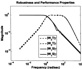
5).

Fig. 10 illustrates the weighted sensitivity and complementary sensitivity W1S and W2T,

corresponding to Csubopt for h = 0.15 and h = 0.25.

Robustness and Performance Properties

10 ..

10.. 10-2 _{10° 10}2 _10•

Frequency (rad/sec)

Figure 10. IW1Shl and IW2Thl for h = 0.25 {red) and h = 0.15 {blue).

Fig. 11 illustrates the effect of the low pass filter connected in series with the optimal controller on the performance level.

-h=0.25 1.5 -h•0.15

!

C 1

r

2 0.5

o~ - -- - ~--..,,._ ___ __

_ _ J 10-5 _{10° 10}5 ₁₀10 Frequency (rad/sec)

A.E. KARAGUL et al.: COMPUTATION OF OPTIMAL 1{.00 _{CONTROLLERS .. . 271}

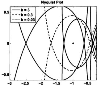
Multiplicative plant uncertainty W2(s) also affects the achievable performance level. In the above discussion, results are obtained for W2(s) = ks, fork= 0.3. To investigate the effect of k, two other choices k

=

0.03 and k

=

3, are considered, and the 1-{X) optimum controller is

computed again. Table 2, shows new ,apt values, and L(s)

=

(as+ l)/(as - 1) functions for

k = 3 and k = 0.03. Figures 12, 13 show the Nyquist plots for the open loop system formed by the optimum controller and the plant for k = 0.03, k = 0.3, and k

=

3, and Table 3 gives gain margin, phase margin, and vector margin values.

Table 2. Calculated "(opt and a values for k

=

0.0~ and k

=

3.

c=5 1.5 1 -1 -1.5 k=3 k = 0.03 I I I h = 0.15 h = 0.25 h = 0.15 h

=

0.25 Nyquist Plot -3 -2 -1 rapt a/b 8.466 11.584 9.981 13.137 0.401 1.352 0.560 1.574 - k = 3 - - -k= 0.3 - k•0.03 0

Figure 12. Nyquist plots of the open loop system fork= 0.03, k

=

0.3, and k = 3, where h = 0.15, and c = 5.

Nyquist Plot

-3 -2.5 -2 -1.5 -1 -0.5

272 APPL. COMPUT. MATH., V.12, N.3, 2013

Table 3. Lower, Upper Gain Margins, Phase Margins, and Vector Margins for k = 0.03, k = 0.3, and k = 3.

Lower GM Upper GM PM k = 0.03 h = 0.15 0.32 2.00 33° h = 0.25 0.40 1.56 25° k =0.3 h = 0.15 0.53 3.13 33° c=5 h = 0.25 0.58 2.13 25° k=3 h = 0.15 0.74 4.45 28.5° h = 0.25 0.78 2.94 22° VM 0.48 0.34 0.57 0.43 0.33 0.27

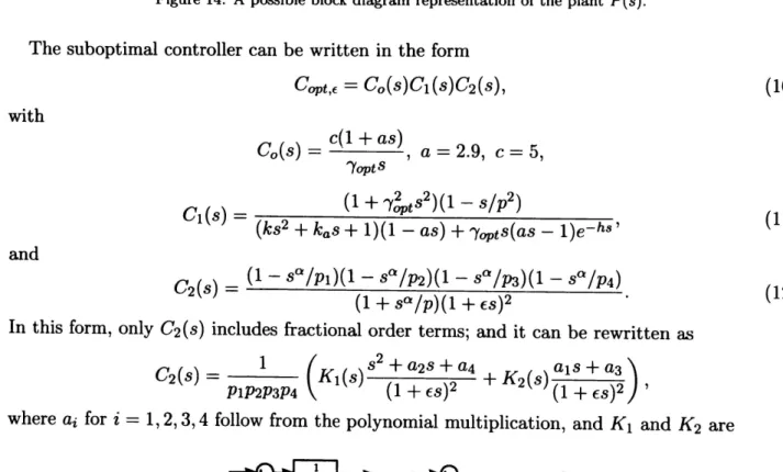
4. IMPLEMENTATION OF THE FRACTIONAL ORDER TERMS

In the previous section, the optimal controller is designed for the non-laminated magnetic suspension system model, derived in

[25].

As seen, both the plant and the controller include fractional order terms. Since fractional terms have infinite memory, approximations to those terms are required for implementation purposes. In the literature, there are continuous, discrete, and frequency response based approximation techniques available, see [47] for an extensive review of these methods. It is observed that to implement both the suboptimal controller and the plant under consideration, it is enough to implement the fractional device ( 1 / s0 ), where O

<

a

<

1.

For example, Fig.14 is a possible block diagram for the plant with (c

=

5)

Figure 14. A po.55ible block diagram representation of the plant P(s) .

The suboptimal controller can be written in the form

Copt ,f

=

Co{s)C1(s)C2{s), with c(l

+

as) C0(s)

=

,

a= 2.9, c

=

5, 'YoptS C1(s)

=

{1

+

'Y~ts2)(1 - s/p2)

(ks2

+

k0s

+

1 ){1 - as)+ 'Yopts(as - 1 )e-hs'

and

c

_2(s)

=

{1 - s0 _{/p1){l - s}0 _{/P2){l - s}0 _{/P3){1 - s}0 _/p4)

{1

+

s0 /p){l

+

_iS)2

In this form , only C2(s) includes fractional order terms; and it can be rewritten as C2(s)

=

1 (K1(s) s2

+

a2s

+

a4

+

K2 s a1s

+

a3)

PIP2P3P4 {1

+

is)2 _{( \1}

+

_{iS)2 '}

where ai for i

=

1, 2, 3, 4 follow from the polynomial multiplication, and K1 and K2 are

K,(•) K,(•)

Figure 15. Block diagram representations for K1(s) and K2(s) .

{10)

{11)

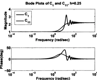
A .E. KARAGUL et al. : COMPUTATION OF OPTIMAL 1i00 _{CONTROLLERS ...} 273

C 1 ( s) has internal unstable pole zero cancellations at s

=

p2 and s

=

±j

h.

After the

cancellations, to approximate

C

1 ( s), the following can be used

1

+

(h/2)s . kap2

C1(s) ~ C11(s) = ₁

+

_(h/2)rcs' where Tc=

}2..1!,

C1(s) = 'Y~t

resulting in the following frequency responses

Bode Plots of C1 and C11 , h=0.15

2

J,·:I~

_{f l}

10""' 10-2 _{10° 10}2 ₁₀4 Frequency (rad/sec)

Jj :

~

I

10""' 10-2 _{10° 10}2 ₁₀4 Frequency (rad/sec)

Figure 16. Bode plots of C1 and C11 .

Bode Plots ofC1 and C11 , h=0.25

iJ ; ~:

I

10""' 10-2 _{10° 10}2 ₁₀4

Frequency (rad/sec)

Figure 17. Bode plots of C1 and C11 .

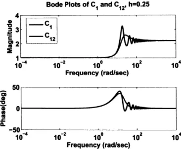
Bode plots of a second degree approximation is depicted in Figures 18 and 19.

1

+

(h/2)s

+

(h2 _/12)s2 Ci(s)

~

Ci2_(s)

=

₁

+

_(h/2)TcS

+

_(h2/12)rcs2 ·

274 APPL . COMPUT. MATH., V .12, N.3, 2013

Bode Plots of C1 and C12, h=0.15

i,.:[~: :

~

l

~o.... 10-2 _{10° 10}2 ₁₀4

Frequency (rad/sec)

Figure 18. Bode plots of C1 and C12

-Bode Plots of C1 and C12, h=0.25

I

~Ii----. ~: I

10.... 10-2 _{10° 10}2 ₁₀4

Frequency (rad/sec)

Figure 19. Bode plots of C1 and C12 .

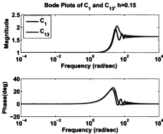
It is possible to increase the order of approximation further, and the third order approximation to C1

1

+

(h/2)s

+

(h2 _/10)s2

+

_(h3 _/120)s3 Ci(s)

~

Ci3_(s)

=

₁

+

_(h/2)TcS

+

_(h2_/lO)TcS2

+

_(h3/120)rcs3 '

A.E. KARAGUL et al.: COMPUTATION OF OPTIMAL 7-f.00 CONTROLLERS ... ₂₇₅ Bode Plots of c1 and c13, h=0.15

nt~J :

i-

I

1~ 1~ 11 1i 11 Frequency (rad/sec)

fj :

2\-

I

1~ 1~ 11 1i 11 Frequency (rad/sec)

Figure 20. Bode plots of C1 and C13.

Bode Plots ofC1 and C13, h=0.25

IJ :

~

I

10~ 1~ 11 1i 11

Frequency (rad/sec)

Figure 21. Bode plots of C1 and C13.

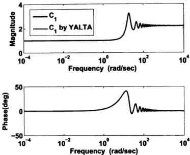
It should also be pointed out that a MATLAB toolbox YALTA can also be used to approximate

C1(s) [2]. A 16th order rational approximation has Bode plots shown in Fig. 22 for h

=

0.15. With this approximation IIC1(s) - C1appr(s)ll00

<

0.083.

lj :

~

I

1~ 1~ 11 1i 11

Frequency (rad/sec)

276 APPL. COMPUT. MATH., V .12, N .3, 2013

In the larger time delay case, a higher order approximation is necessary to keep the er~or between frequency responses similar. Therefore, for h

=

0.25, a 36th order transfer function is used to approximate C1. Fig. 23 illustrates its frequency response, with the error IIC1(s) -C1appr(s)lloo

<

0.13. 4 . - - - , - - - . . - - - - ~ - - - , ~ --C1 :,

!

2 - - C₁ by YALTA

i'

2 0 ' ~ ~ ~ -10""" 10-2 _{10° 10}2 _10' Frequency (rad/sec)

tJ :

~

I

10""" 10-2 _{10° 10}2 _10' Frequency (rad/sec)

Figure 23. Bode plots of C1 and its approximation by YALTA, for h

=

0.25 .

In the remaining parts of this section, some approximation techniques for the fractional order term of the controller are reviewed, and a new approximation technique based on frequency response data is proposed. In the following part, FIR representation of a fractance device (1/s0 ) will be given~ and this will be followed by continuous approximation techniques, namely

Matsuda's method and Carlson's method. Finally, a frequency response data approximation technique MATLAB's invfreqs command will be performed, followed by the proposed algo-rithm.

. . . ... · :..

4.1. FIR Implementation of Fractance Device. This part deals with the FIR implementa-tion of the fractance device (1/ s0 ) , where O

<

o

<

l. In order to get coefficients of the filter, the impulse invariance method is used. First, the inverse Laplace transform of the fractance device is obtained

1 ,/irt"

Then the corresponding FIR filter , through z-1

=

_{e-sT transformation is} H1(s)

=

Z {K

ff.

[ho,_!_,_!_, .. . , -

1 ] } where ni

=

Vi

V;

n1 n2 nN

K . _{1s constant gam,} . h _{0 :=} 1· _1m l _{r,;;, i} . _{= 1, 2, ... , N ;}

n--o vn

we take N

=

2000 for good precision in the approximation, and sampling time T

=

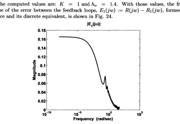
0.01 sec. In this filter, since the first coefficient cannot be computed, to minimize the error between the feedback loops formed by the fractance and its impulse invariant equivalent, a constant gain (K) and a constant coefficient (h0 ) are used [23] . For this purpose, we minimize

ll(R(s) - R1( s)) s0

llx ,

_{where R1(s)}

=

_{Hi(s~ ) , and R( s )}

= - .-

1

A.E. KARAGUL et al.: COMPUTATION OF OPTIMAL H.00 _{CONTROLLERS ... 277}

Then the computed values are: K = 1 and h0 = 1.4. With those values, the frequency

response of the error between the feedback loops, E1(jw) := R(jw) - R1(jw), formed by the fractance and its discrete equivalent, is shown in Fig. 24.

0.16 0.14 0.12 IE10ro)I QI 'ti ,a 0.1 ·2

:f

0.08 :I! 0.06 0.04 0.02 o ~ - - - - ~ - - - - ~ - ~ - - _ _ . 10-10 _{10-5 10° 10}5 Frequency (rad/sec)

Figure 24. Frequency response of the error E1 (s).

It is also possible to obtain continuous time representation of the FIR filter . Define state space representation of the FIR filter

x[n

+

1 J

=

Ax[n]

+

Bu[n],

y[n]

=

Cx[n]

+

Du[n], where A, B, C, D are: Define H2(s) to be

[010···0]

0 0 1 · · · 0

[OJ

0

A= B=

b b

O .... :

b

NxN'

i

Nxl,

C

=

J!K

[hN, hN-1, · · · hi] lxN, D=

/rho.

H2(s)

=

Cc(J - e-h(sl-A,,))(sl - Ac)-1 _{Be+ De.}

Then, H2(s) is a transfer function with FIR filter behavior. To get Ac, Be, Cc , De from A, B, C, D, bilinear transformation is used

. t ad f 1 +sT /2 h

ms e o z, put l-sT/2 , t en

zX=AX+BU,

278 APPL . COMPUT. MATH., V.12, N.3, 2013

Ac= ~(A - I)(A

+ /)-

1 , T

Be=

Jr

(B -

(A - I)(A

+ /)-

1

_B),

Cc= Jrc(A

+ /)-

1 ,

Dc=D-C(A+I)-1_B.

After obtaining continuous time representation of the filter the model reduction scheme pro-posed in [21] is used. Here, N is reduced from 2000 to 80. The approximate transfer function is calculated.

Let E2(s)

=

R(s) - _{R2(s), where R2(s)}

=

H2(s)/(l

+

H2(s)). The error E2(jw) is illustrated in Fig. 25. IE20ro )I 0.18 0.16 0.14 0.12

•

,,

0.1 ~ ~ C

i'

0.08 ::& 0.06 0.04 0.02 0 10-10 10-5 _{10° 10}5 Frequency (rad/sec)

Figure 25. Frequency response of the error E2(s).

4.2. Continuous Approximation Methods. The fractional order term in the controller,

C2(s), recall (12) contains irrational functions of the Laplace variables, and in this part, rational approximations are investigated. This section reviews two methods: Matsuda's Method, and Carlson's Method. Both of the methods are evaluated in such a way that they both produce a transfer function where the degree of the approximation is 15.

In

[29],

a method is proposed to obtain a rational function approximating an irrational one. This method uses continued fraction expansion, and logarithmically spaced w values to fit the original function with s -wo H3(s)

=

ao

+

-s -w1 a 1 + -s-w2 a 2 + -a3

+ ...

S -Wi

Vo(s) := H(s), ai

=

Vi(wi), Vi+I

=

.

t\(s) - ai

A.E. KARAGUL et al. : COMPUTATION OF OPTIMAL 'H.00 _{CONTROLLERS ... 279}

We performed this method over the internal w E (10-5 , 105 ) with a transfer function degree constraint of 15. This gives the third alternative approximation H3(s). Then we define E3(s)

=

R(s) - H3(s)/(l

+

H3(s)). Fig. 26 illustrates the frequency response of E3(s).

-3 1_2 X 10 1 -0.8 .g :I

i

0.6 CII

..

:I! 0.4 0.2 o ~ - - ~ - - ~ ~ - - ~ - - ~ 10-20 _{10-10 109 1019 10}20 Frequency (rad/sec)

Figure 26. Frequency response of the error E3(s) .

To approximate the fractional order terms (s°'), Carlson's method can also be used [12].

Defining the function H4(s)

=

(G(s))°', in this case G(s)

=

1/s, starting with F0(s)

=

1,

iteration follows

(q - m)(Fi-1(s))2

+

_(q

+

_m)G(s)

Fi(s) = Fi-1(s) ( )(F: ( ))2 ( )G( ) , where, a= 1/q, m = q/2. q

+

m i-1 s

+

q - m s

By this method, an approximate transfer function H4(s) with degree 15, is obtained. Fig.

27 shows the error IE4(jw)I between the feedback loops, where E4(s)

=

R(s) - ~(s), and

R4(s)

=

H4(s)/(l

+

H4(s)). IE4(i<,>)I 0.04 0.035 0.03 _g 0.025

.a

c 0.02 CII

..

:I! 0.015 0.01 0.005 0 10-10 10-5 10° 105 ₁₀10 Frequency (rad/sec)

Figure 27. Frequency response of the error E4(s).

4.3. Frequency Response Based Approximation Method. Performing invfreqs on the frequency response data of the actual feedback loop with weighting function W(s)

=

(1

+

s/T1)/(l

+

s/T2)2, where T1

=

3 x 10-5 _and T2

=

1. Now consider R(s)

=

R(s) I+ s/T1

280 APPL. COMPUT. MATH., V.12, N.3, 2013

and obtain R(jw) for w values in (10-5, 105). Now apply invfreqs, this gives an approximation

n

5(s) of degree 18. Define E 5(s)

=

R(s) - H5(s). The magnitude of E5(s) is given in Fig. 28.

fE50ro)I 0.09 0.08 0.07 0.06

•

"g 0.05

-=

C lf0.04 :I 0.03 0.02 0.01 0 10-11 _{10-s 10}1 105 Frequency (rad/sec)

Figure 28. Frequency response of the error Es(s) .

4.4. An Alternative Approximation Method. In order to realize a fractional order system

model G(s0 ) (where in our study we consider G(s0 )

=

1/

Js),

to make it implementable in

simulation environments, it must be approximated by a finite dimensional system Gapp(s). For this objective, an identification algorithm is proposed. This algorithm uses a pre-defined basis function in the form of a first degree transfer function in s-domain, which has a relative degree of zero. For more general classes of G(s0 ) , a different basis may be used. We choose the basis given in (13), so that the rational approximation of the fractional device has real poles and zeros, as. in ~~V.4~:s _method

[42].

The basis function can be constructed as

. . . ...

ft.···~~~-. · ·•• ··ft.···~~~-. '' • ( ) ak 1 s

+

ak o

9k s

=

'

'

bk,IS

+

bk,O' (13)

wheres is the Laplace variable, and ak,I, ak,O, bk,I, bk,O are real parameters. Overall, the transfer

function is the product of these basis functions. The final aim is to construct a transfer function of the form

l

N

Js

~

GN(s)

=

IT

9k(s),

k=l

(14)

where 9k(s) is defined as in (13). The target constrained optimization problem for the purpose of approximating a transfer function in s0-domain is defined below.

~I¢?· -

G N(J·w· 0)

1

2 mini₈mize c(!l.)

=

~

'

.

'' -

,

- i=l GN(JWi,!l.) subject

to

fl.

~ 0, (15) (16)

where

¢?i

is the value of the transfer function in s0_{-domain at} jwi, G(jw)

=

G(s)ls=jw

_{is given}

as in (14), Wi are distinct frequency points which do not need to be uniformly spaced,

fl.

is the parameter vector, and ~ means element-wise inequality of a vector

[25].

More precisely,

A.E. KARAGUL et al.: COMPUTATION OF OPTIMAL ?-f.<X> CONTROLLERS ... 281

(17)

ai,j 2 0 and bi,j 2 0, V(i,j), i

=

1,2 ... N and j

=

1,2.

Optimization problem (15), targets minimizing the relative error between two different transfer functions, containing nonlinear properties owing to the selected type of functions, which are ratios of two complex polynomials. In the direction of fitting a transfer function in the s-domain with the fewest possible number of parameters, a nonlinear least squares (NLLS) approach is preferred. The NLLS method also gives a good optimized result, as illustrated below.

The parameters of the 15th order approximation in the form (13), are shown in the table below. Now define H6(s)

=

G1s(s). Then, E6(s)

=

R(s) - H6(s)/{1

+

H6(s)).

(Ji values (where MATLAB notation e-2 is used for 10-2).

k 1 2 3 4 5 6 7

Ok,! 17.7098 11.2916 11.2933 11.3453 11.3494 11.9345 14.2194 Ok,O 0.0206e-02 0.0785e-02 0.4171e-02 11.692e-02 2.2146e-02 64.952e-02 4.0869 bk,I 8.8974 13.3577 13.3498 13.3064 13.1025 12.8254 14.4704 bk,O 0.0026e-02 0.0396e-02 0.2144e-02 l.1300e-02 5.8760e-02 30.374e-02 1.8098

k 9 10 11 12 13 14

Ok,! 2.3805 2.2812 2.1827 2.0881 1.9957 0.1902 Ok,O 0.1908e+02 0.9657e+02 4.8802e+02 24.658e+02 124.59e+02 629.50e+02 bk,I 5.2973 5.2360 5.0156 4.7983 4.5889 4.3669 bk,O 0.18479e+02 0.96462e+02 4.8800e+02 24.658e+02 124.59e+02 629.50e+02

The resulting error is shown in Fig. 29.

Q) -3 1_6

x

10 1.4 1.2 't, 1 ::::,

-·2 0.8 C>

i

0.6 0.4 0.2 o ~ c . _ _ - - - ~ - - - ~

1~

1i

1~

Frequency (rad/sec)

Figure 29. Frequency response of the error E6(s).

5. TIME DOMAIN SIMULATION RESULTS

8 22.0645 0.3349e+02 33.2663 0.2197e+02 15 2.9590 1000.0e+02 1.1643 1000.0e+02

In this section, time domain simulation results for the feedback system formed by the

,txi

controller and the non-laminated magnetic suspension system plant model, are illustrated by using the approximation and implementation techniques presented in Sections 4 and 5.

The plant is implemented as shown in Fig. 14. The suboptimum controller is implemented according to equation 10. For the fractional order terms in the plant, and in C2(s), a 15th degree approximation, obtained from the proposed method of Section 4.4, is used. To approximate

282 APPL. COMPUT. MATH., V.12, N.3, 2013

Ci (s), YALTA toolbox is used. For h.

=

0.1~, a 16th degree .transfer function, and for h

=

0.25, a 34th degree approximate is used. S1mulat1ons are done usmg MATLAB.

Fig. 30 illustrates the step response of the closed loop systems for h = 0.15, and fork= 0.03, k

=

3, and k

=

0.3.

Step Response of the Closed Loop System

3-~-.---.---.---:======;i - - -k = 0.3 2.5 : 2 C 0 a.

I

1.5 a:: a. ; 1 0.5 5 10 15 Time in sec. -k=0.03 - k = 3 20 25

Figure 30. Step response of the closed loop system for h

=

0.15, without any disturbance.

Fig. 31 illustrates the step responses of the closed loop system for h

=

0.25, and for k

=

0.03,

k

:=:

i~.Jwi

~J~~~

.

·-.~..'.:.-J,,~---Step Response of the Closed Loop System

3.5,---r---.--..,...---r;:::::====:::;1 3 CD 2.5 en C

&.

2 Ill ~ a. 1.5

;

1 0.5 - - -k = 0.3 -k=0.03 - k = 3 5 10 15 20 25 30 Time in sec.

Figure 31. Step response of the closed loop system for h = 0.25, without any disturbance.

To investigate the effect of the disturbance, the magnitude of the transfer function from disturbance to output is calculated, as shown in Fig. 32. At the frequency (wd) where the magnitude is highest, a sinusoidal disturbance in the from sin(wdt), is applied to the system. Therefore, the maximum disturbance that can be observed at the output is simulated, as shown in Figures 34 and 35. Furthermore, step disturbance is also applied to the system, and the resulting output is depicted in Figures 36 and 37.

A.E. KARAGUL et al.: COMPUTATION OF OPTIMAL 1-(.'Xl CONTROLLERS ...

-

:::,

s-

_:::,

10°

Frequency Response of Tyd

- - -k = 0.3

10"""

1 0 - 1 2 ~ - - - ~ - - - ~ - - - - ~ - - - _ J

10""" 10-2 _{10° 10}2 ₁₀4

Frequency (rad/sec)

Figure 32. ITydl, for h

=

0.15.

Frequency Response of Tyd

1 0 - 1 2 ~ - - - ~ - - - ~ - - - - ~ - - - ~ 10""" 10-2 _{10° 10}2 ₁₀4 0.4 0.2 0 Frequency (rad/sec)

Figure 33. ITydl, for h

= 0.25.

Output to Sinusoidal Disturbance

0 -0.2 -0.4 -0.6 10 20 Time in sec. 30 40

Figure 34. Maximum disturbance that can be observed at the output for h = 0.15.

284

I

APPL. COMPUT. MATH ., V.12, N .3, 2013

Output to Sinusoidal Disturbance

0·8 - - -k"' 0.3 0.6 - - k = 0.03 --k=3 0.4 0.2 -0.2 -0.4 -0.6 -0.80 10 20 30 40 50 Time In sec.

Figure 35. Maximum disturbance that can be observed at the output for h

=

0.25.

iz~ -is. :~:. ·: ~.-.: •· ;. :. · 0.35 0.3 0.25 "S _Cl. 0.2 "S 0.15 0 0.1 0.05 0 -0.050 5

Output to Step Disturbance

10 15 Time In sec. - - -k= 0.3 - k = 0.03 - k = 3 20 25

Figure 36. Output to step disturbance for h

=

0.15.

Output to Step Disturbance

0.6 0.5 - - -k = 0.3 -k=0.03 0.4 - k = 3 "S 0.3 Cl. "S 0 0.2 0.1 0

-o

11

·o

_{5 10 15 20 25 30} Time in sec.

Figure 3i. Output to step disturbance for h

=

0.25.

To sec the effect of the multiplicative plant uncertainty bound on the robustness , the graphs of II/Try(jw)l - 1 _{versus ;JJ arc given in Figures 38 and 39. It can be observed that for fast step}

A .E. KARAGUL et al.: COMPUTATION OF OPTIMAL ?i.00 CONTROLLERS ... 285

responses, k should be small, however, that leads to poor robustness levels as illustrated in Figures 38 and 39.

Frequency Response ofTyr

101 ~ - - ~ - - - ~ - - - ~ - - - - , ---k=0.3 -k:z0.03 - k = 3 10-2 ~ - - ~ - - - ~ - - - ~ - - - - ' 10-4 10~ 11 1i 1~ Frequency (rad/sec:)

Figure 38. ITyr(sW1 , for h

=

0.15.

Frequency Response of Tyr

101 ~ - - ~ - - - ~ - - - ~ - - - - , - - -k •0.3 -k=0.03 - k : 3 10-2 ~ - - ~ - - - ~ - - - ~ - - - - ' 10-4 10-2 _{10° 10}2 _10' Frequency (rad/sec:)

Figure 39. ITyr(sW1 , for h

=

0.25.

6. CONCLUSION

In this work, some recent techniques in fractional order systems are reviewed, and as a design example, the 1{.00 optimal controller is designed for a fractional order system. Then various

approximation methods are discussed for the implementation of the optimal controller.

Definitions of fractional order integration and differentiation are recalled from the literature. An example on the Bode's ideal open loop transfer function is given to illustrate a desirable property of fractional order systems. Recently, in a series of papers [25, 49], a mathematical model of the non-laminated magnetic suspension system is obtained. This model includes frac-tional order terms along with a time delay. For such infinite dimensional plants, the method in [44] can be used to compute the 1{.00 optimal controller. When the weights are low order,

the method can be simplified, as given in [36]. This paper computes the ,tw optimal controller

286 APPL. COMPUT. MATH., V.12, N.3, 2013

time delay on the achievable performance level is illustrated. To investigate t~e effect of the multiplicative plant uncertainty bound W2(s) on the performance level, the optimal controller

is designed for three different weighting functions, and the results are given. To implement the fractional order term in the controller, some approximation techniques are performed, and a new approximation method is proposed. For illustrative purposes, time domain simulation results are given for different delay and uncertainty levels.

REFERENCES

(1) Astrom, K.J . Limitations on Control System Performance, Preprint, 1999.

(2) Avanessoff, D., Bonnet, C., Fioravanti, A., Nguyen L.H.V. User document YALTA, https ://gforge . inria.fr/projects/yalta-toolbox, January 2013.

(3) Bohannan, G.W. Analog realization of a fractional controller, revisited, In: BM Vinagre, YQ Chen, eds,

Tutorial Workshop 2: Fractional Calculus Applications in Automatic Control and Robotics, Las Vegas, USA, 2002.

(4) Bohannan, G.W. Analog realization of a fractional control element-revisited, In IEEE CDC2002 Tutorial Workshop, Las Vegas, NE, USA, V.27, 2002.

(5) Bonnet, C., Fioravanti, A.R., Partington, J .R. Stability of neutral systems with commensurate delays and poles asymptotic to the imaginary axis, SIAM Journal on Control and Optimization, V.49, 2011, pp.498-516. (6) Boyd, S.P., Vandenberghe, L. Convex Optimization, Cambridge University Press, 2004.

(7) Bydder, M. Solution of a complex least squares problem with constrained phase, Linear Algebra Appl., V.433, N.(11-12), 2010, pp.1719-1721.

(8) Calderon, A.J., Vinagre, B.M., Feliu, V. Linear fractional order control of a DC-DC buck converter, Pro-ceedings of European Control Conference, Cambridge, UK, 2003.

(9) Caputo, M. Linear models of dissipation whose Q is almost frequency independent - II, Geophysical Journal International, V.13, N.5, 1967, pp.529-539.

(10) Caputo, M., Elasticita e Dissipacione, Bologna: Zanichelli, 1969.

(11) Carlson, G.E. and Halijak, C.A. Approximation of fractional capacitors (1/s)1_{/n by a regular Newton process,}

IEEE '.lhinsactions on Circuit Theory, V.11, 1964, pp.210-213.

(12) Carlson, G.E., Halijak, C.A., Approximation of fractional capacitors (l/s)1 /" by a regular Newton prm;e;i;,

IRE TI-ansactions on Circuit Theory, CT-11, N.2, 1964, pp.210-213.

(13) Chen, Y.Q., Moore, K.L. Discretization schemes for fractional-order differentiators and integrators, IEEE TI-ans . Circuits Syst. I Fundam. Theory Appl., V.49, N.3, 2002, pp.363-367.

(14) Domek, S. Switched state model predictive control of fractional-order nonlinear discrete-time systems, Asian Journal of Contro~ V.15, 2013, pp.658-668.

(15) Doyle, J.C., Francis, B.A., Tannenbaum, A. Feedback Control Theory, New York: Macmillan Publishing Company, 1992.

(16) Ferreira, N.F., Machado, J.T. Fractional-order hybrid control of robotic manipulators, In Proceedings of the 11th International Conference on Advanced Robotics, July 2003.

(17) Fioravanti, A.R., Bonnet, C., Ozbay, H. Stability of fractional neutral systems with multiple delays and (18) (19) [20) (21) (22) (23) [24] [25] [26)

poles asymptotic to the imaginary axis, In 49th IEEE Conference on Decision and Control, December 2010, pp.31-35.

Fioravanti, A.R., Bonnet, C., Ozbay, H., Niculescu, S.I. A numerical method for stability windows and unstable root-locus calculation for linear fractional time-delay systems, Automatica, V. 48, pp.2824-2830. Fioravanti, A.R., Bonnet, C., Ozbay, H., Niculescu, S-1. Stability windows and unstable root loci for linear fractional order systems, The 18th /FAG World Congress, Milan, Italy, 2011, pp.12532-12537.

Fioravanti, A.R. , Bonnet, C. , Ozbay, H., Niculescu, S.I. Stability windows and unstable poles for linear time-delay systems, 9th IFAC Workshop on Time-Delay Systems, Prague, June 2010.

Gu, G., Khargonekar, P.P., Lee, E.B. Approximation of infinite-dimensional systems, IEEE TI-ansactions on Automatic Contro~ V.34, N.6, 1989, pp.610-618.

Hamamci, S.E. An algorithm for stabilization of fractional-order time delay systems using fractional-order PID controllers, IEEE TI-ansactions on Automatic Control, V.52, N.10, 2007, pp.1964-1969.

Jackson, L.B. A correction to impulse invariance, IEEE Signal Processing Letters, V.7, N.10, 2000, pp.273-275.

Jiao, Z., Chen, Y., Zhong, Y. Stability analysis of linear time-invariant distributed-order systems, Asian Jounmal of Control, V.15, 2013, pp.640-647.

Knospe. C'.R .. Zhu, L. Performance limitations of nonlaminated magnetic suspension systems, IEEE Trans. on Control Systems Technology, V.19, N.2, 2011, pp.327-336.

Lan. Y.-H. , Zhou . Y. D0_{-type iterative learning control for fractional-order linear time-delay systems.}

Asian Journal of Control. V.15. 2013. pp.669-6ii.

A.E. KARAGUL et al.: COMPUTATION OF OPTIMAL H00 _{CONTROLLERS .. . 287}

(27) Lourakis, M.I. A Brief Description of the Levenberg-Marquardt Algorithm Implemented by Levmar, Institute of Computer Science, Foundation for Research and Technology, 2005.

[28) Matti, R., Aoun, M., Cois, 0., Oustaloup A, and Levron F. H2-Norm of fractional differential systems. Proceedings of the ASME 2003 Design Engineering Technical Conferences and Computers and Information in Engineering Conference, Chicago, USA, DETC2003/V18-48387, 2003.

(29) Matsuda, K. and Fujii, H. 1t00-optimized wave-absorbing control: analytical and experimental results,

Jour-nal of Guidance, Control, and Dynamics, V.16, 1993, pp.1146-1153.

[30) Miller, K.S., Ross, B. An Introduction to the Fractional Calculus and Fractional Differential Equations, John Wiley and Sons, New York., 1993.

[31) Monje C.A., Chen Y.Q., Vinagre B.M ., Xue D., and Feliu V. Fractional-Order Systems and Controls: Fun-damentals and Applications, London, Springer, 2010.

[32) Monje, C. A. , Ramos, F ., Feliu, V., Vinagre, B.M. Tip position control of a lightweight flexible manipulator using a fractional order controller, JET Control Theory & Applications, V.l, N.5, 2007, pp.1451-1460. [33) Oustaloup, A. Complex non integer derivation in robust control through the CRONE control, In Analysis of

Controlled Dynamical Systems Progress in Systems and Control Theory, V.8, 1991, pp.326-336.

[34) Oustaloup, A., Levron, F ., Mathieu, B., and Nanot, F.M. Frequency-band complex noninteger differentiator: Characterization and synthesis, IEEE '.lransactions on Circuit and Systems - I: Fundamental Theory and Application, V.47, 2000, pp.25-39.

[35) Oustaloup, A., Mathieu, B., Lanusse, P. The CRONE control of resonant plants: application to a flexible transmission, European Journal of Control, V.l, N.2, 1995, pp.113-121.

[36) Ozbay, H. Computation of 1t00 _{controllers for infinite dimensional plants using numerical linear algebra,}

Nu.mer. Linear Algebra Appl, V.20, 2013, pp.327-335.

[37) Ozbay, H., Bonnet, C., Fioravanti, A.R. PID controller design for fractional-order systems with time delays, Systems & Controller Letters, V.61, 2012, pp.18-32.

[38) Padula, F ., Visioli, A., Set-point weight tuning rules for fractional-order PID controllers, Asian Journal of Control, V.15, 2013, pp.678-690.

[39) Petras, I., Hypiusova, M. Design of fractional-order controllers via 1t00 norm minimisation, Selected Topics

in Modelling and Control, V.3, 2002, pp.50-54.

[40) Petras, I. , Podlubny, I., O'Leary, P. Analogue Realization of Fractional Order as Controllers, Fakulta BERG, TU Kosice, 2002.

[41] Podlubny, I. Fractional differential equations, MatJ,ematics in Science and Engineering, V.198, Academic Press, San Diego, 1999.

[42] Podlubny, I. Fractional-order systems and PI>, Dµ controllers, IEEE '.lransactions on Automatic Control, V. 44, 1999, pp.208-214.

[43) Pommier-Budinger, V., Musset, R., Lanusse, P., Oustaloup, A., Study of two robust controls for an hydraulic actuator, in European Control Conference, Cambridge, United Kingdom, 2003.

[44] Toker, 0., Ozbay, H. 1t00 optimal and suboptimal controllers for infinite dimensional SISO plants, IEEE

Transactions on Automatic Control, V.40, 1995, pp.751-755.

[45) Valerio, D., Fractional robust system control, Ph.D. Thesis, Instituto Superior Tecnico, Universidade Tecnica de Lisboa, 2005.

[46] Valerio, D., Sada Costa, J. Variable Order Fractional Controllers, Asian Journal of Control, V.15, 2013, pp.658-657.

[47] Vinagre, B. M., Podlubny, I., Hernandez, A., Feliu, V. Some approximations of fractional order operators used in control theory and applications, Fractional Calculus and Applied Analysis, V.3, 2000, pp.231-248. (48] Wang, D.-J ., Gao, X.-L. Stability Margins and 1t00 Co-Design with Fractional-Order PI>,Controllers, Asian

Journal of Control, V.15, 2013, pp.691-697.

(49] Zhu, L., Knospe, C.R. Modeling of nonlaminated electromagnetic suspension systems, IEEE/ASME '.lrans-actions on Mechatronics, V.15, 2010, pp.59-69.

288 APPL. COMPUT. MATH., V.12, N.3, 2013

Erdem Karagul - is a master's student at

Bilkent University, with an emphasis in systems and control. He works under the supervision of Prof. Hitay Ozbay. He is a graduate of Gazi Ana-tolian High School and received his B.S. degree from Bilkent University.

Okan Demir - received his B.S. degree in

Elec-trical and Electronics Engineering from Mersin University, Turkey. Currently, he is a graduate student at Bilkent University, under supervision of Prof. Hitay Ozbay. His research interest are in signals, systems and control.

Hitay Ozbay - received his B.S. degree in

Electrical Engineering from Middle East Techni-cal University (Ankara, Turkey) in 1985, M.Eng degree in Electrical Engineering from McGill Uni-versity (Montreal, Canada) in 1987, and Ph.D . de-gree in Control Sciences and Dynamical Systems from the University of Minnesota, (Minneapolis, USA) in 1989.He was an Assistant Professor of Electrical Engineering at the University of Rhode Island from September 1989 to December 1990. He was with the The Ohio State University (1991-2006) where he was a Professor of Electrical and Computer Engineering, prior to joining Bilkent University in 2002, on leave from OSU.

He was an Associate Editor on the Editorial Board of the IEEE Transactions on Automatic Control (1997-1999) , and was a member of the Board of Governors of the IEEE Control Systems Society ( 1999 and 2013). He served as an Associate Editor of Automatica (a journal of International Federation of Automatic Control) , 2001-2007, and as a vice-chair of the Technical Committee Networked Control Systems of IFAC, 2005-2011. Currently, he is an Associate Editor for SIAM Journal on Control and Optimization, and for Automatica.

Appl. Comput. Math., V.12, N.3, 2013, pp.289-305

EFFICIENCY OF COMBINED DAUBECHIES AND STATISTICAL PARAMETERS APPLIED IN MAMMOGRAPHY

M. ASADZADEHt.t, E. HASHEMI 1 •2 , A. KOZAKEVICIUS 1,3,t ,•

ABSTRACT. The proposed methodology combines a Daubechies (Db2) wavelet transform, and the statistical parameters, skewness, and kurtosis for the detection of microcalcifications in mam-mography. The efficiency of the discrete algorithm is heavily relied on the order of performing wavelet approximation and the computation of the statistical moments. The significance of wavelet and statistical parameter approaches, as well as the ordering issue in performing the analysis, are justified through implementing numerical examples for some clinical data. Finally, a ROC curve summarizing the performance of the CAD scheme is also presented.

Keywords: Daubechies Wavelet, Vanishing Moments, Mammography, Microcalcification, Skew-ness, Kurtosis.

AMS Subject Classification: 65T60, 68UI0, 97K80, 97M60.

1. INTRODUCTION

Mammography is a common expression for a specific type of imaging that uses a low-dose x-ray (photon-beam) to examine breast tissue, and a mammography exam is called a mammogram [3]. One of the main indicators of breast cancer searched in mammograms, is a set of clusters formed by microcalcifications (also denoted by µCa++). These are tiny calcium deposits in breast tissue, that appear as small bright spots in the imaging [3, 13].

Computer-aided diagnosis (CAD) methods are now widely used for the detection of breast mi-crocalcifications. Already back in the 80's, Chan and collaborators [4, 5] introduced a difference-image approach using a matched filter /box-rim filter combination to remove the structured back-ground from the images. Also, techniques based on gray-level thresholding or signal-extraction, adapted to the known physical characteristics of microcalcifications, were used to isolate mi-crocalcifications from the noise in the background. The CAD system aims to produce a kind of "second opinion" for the radiologist's use, improving the accuracy in detecting clustered mi-crocalcifications [10, 11] . Reductions in computer's false-positive rates may further improve radiologist 's diagnostic accuracy. To this end, wavelet methods were incorporated to CAD schemes in different ways, in order to analyze and pre-process the images. In this regard, Mon-ica Penedo et al [26] employed wavelets to compress regions of interest (ROI) in mammograms, which were diagnostic relevant, and obtained segmentation of the compressed images using a border detection technique. Whereas Lado et al [16, 22] considered instead wavelets as part of the classification stage of the designed CAD scheme.

Microcalcifications in mammograms correspond to high frequency coefficients of the image spectrum, see e.g. [17, 29]. An easy procedure to detect and extract these microcalcifications

1 _{Chalmers University of Technology, Sweden, e-mail: [email protected]}

2 _{Polytechnic de Torino, Italy, e-mail: [email protected]}

3 _{Universidade Federal de Santa Maria - UFSM, Brazil, e-mail: [email protected]}

t The research of this author is supported by the Swedish Foundation of Strategic Research (SSF) in Gothen-burg Mathematical Modeling Center (GMMC) and Swedish Research Council (VR).

* The author is supported by the grant No 201457 /2010-5 of the National Counsel of Technological and Scientific Development - CNPq (Brazil) .

Manuscript received 29 September 2012.