The design of finite-state machines for quantization using simulated annealing

A THESIS

SUBMITTED TO THE DEPARTMENT OF ELECTRICAL AND ELECTRONICS ENGINEERING

AND THE INSTITUTE OF ENGINEERING AND SCIENCES OF BILKENT UNIVERSITY

IN PARTIAL FULFILLMENT OF THE REQUIREMENTS FOR THE DEGREE OF

MASTER OF SCIENCE

By

Ercan Engin Kııruoğlıı

August 1993

■^6·} ' i Э 9'^

I certify that I have read this thesis and that in my opinion it is fully adequate, in scope and in quality, as a thesis for the degree of Master of Science.

Assoc. Prof. Dr. Ender Ayanoglu (Principal Advi.sor)

I certify that I have read this thesis and that in my opinion it is fully adequate, in scope and in quality, as a thesis for the degree of Master of Science.

Assüc. Prof. Dr. Erdal Ankan

I certify that I have read this thesis and that in my opinion it is fully adequate, in scope and in quality, as a thesis for the degree of Master of Science.

i .

Assoc. Prof. Dr. Enis Çetin

Approved for the Institute of Engineering and Sciences:

Prof. Dr. Mehmet

THE DESIGN OF FINITE-STATE MACHINES FOR

QUANTIZATION USING SIMULATED ANNEALING

Ercaii Eiigin Kuruoglii

M.S. in Electrical and Electronics Engineering

Supervisor: Assoc. Prof. Dr. Ender Ayanogiu

August 1993

In this thesis, the combinatorial optimization algorithm known as simulated an­ nealing (SA) is applied to the solution of the next-state map design problem of data compression systems based on finite-state machine decoders. These data compression systems which include finite-state vector ciuantization (FSVQ), trellis waveform coding (TWC), predictive trellis waveform coding (PTWC), and trellis coded quantization (TCQ) are studied in depth. Incorporating gen­ eralized Lloyd algorithm for the optimization of output map to SA, a finite-state machine decoder design algorithm for the joint optimization of output map and next-state map is constructed. Simulation results on several discrete-time sources for FSVQ, TWC and PTWC show that decoders with higher per­ formance are obtained by the SA-I-CLA algorithm, when compared to other related work in the literature. In TCQ, simulation results are obtained for sources with memory and new observations are made.

Keywords : data compression, Jlnitc-state vector quantization, trellis waveform coding, predictive trellis xvaveform coding, trellis coded quantization, simulated annealing, finite-state machine decoders.

TAVLAMA BENZETİMİ KULLANARAK NİCEMLEME

AMAÇLI SONLU DURUM MAKİNELERİ TASARIMI

Ercan Engin Kuruoğlu

Elektrik ve Elektronik Mühendisliği Yüksek Lisans

Tez Yöneticisi: Doç. Dr. Ender Ayanoğiu

Ağustos 1993

Bu çalışmada, sonlu durum makinelerine dayanan bazı veri sıkıştırma dizgelerinde eniyiye yakın kodçözûcü tasarımı sorununa bir çözüm önerisi irdelenmiştir. Tezin bu konudtiki araştırmalara temel katkısı, kodçözücü durum değiştirme tablosu tasarımında tavlama benzetimi olarak bilinen katışımsal eniyileştirme algoritmasının kullanılmasıdır. Çıktı tablosunun eniyi- leştirilmesinde kullanılan genelleştirilmiş Lloyd algoritması da tavlama ben­ zetimi ile birlikte çalıştırılarak çıktı tablosu ve durum değiştirme tablosunu beraber eniyileştiren bir tasarım algoritması oluşturulmuştur. Sonlu durum vektör nicemleyicisi, çit kaynak kodlaması ve öngörülü çit kaynak kodla­ ması için elde edilen benzetim sonuçları önerilen algoritma ile daha önce yayınlanmış çalışmalara göre daha yüksek başarımlı kodçözücülerin tasar­ landığını göstermektedir. Çit kodlamalı nicemleme için de yeni gözlemlerde bulunulmuştur.

Anahtar sözcükler : veri sıkıştırma, sonlu durum vektör nicemleyicisi, çit kaynak kodlaması, öngörülü çit kaynak kodlaması, çit kodlamak nicemleme, tavlama benzetimi, sonlu durum makineli kodçözücü.

I would like to thank Dr. Ender Ayanoğlu for his supervision, guidance and suggestions during the development of this thesis. I would like to thank Dr. Erdal Arikan for many invaluable discussions. I would also like to thank him and Dr. Ellis Çetin for reading and commenting on the thesis.

My special thanks go to Sarah (Clay) for her love, patience, understanding and encouragement especially at times of hardship and despair. Of course, I cannot pass without mentioning my parents and my sister here, whose very existence gave me so much courage.

I would like to extend my thanks to Dr. İlknur Özgen and Dr. Varol Akman for their support and closeness. And the last but by no means the least, my sincerest feelings are towards all of my friends for the times we had.

1 INTRODUCTION 1

2 QUANTIZATION TECHNIQUES 4

2.1 Scalar Q u an tizatio n ... 4

2.2 Vector Quantization 6 2.3 Finite-State Vector Quantization 8 2.4 Trellis Waveform C o d in g ... 14

2.4.1 Viterbi A lgorithm ... 18

2.5 Predictive Trellis Waveform C o d in g ... 19

2.5.1 System D escrip tio n ... 20

2.5.2 Search A lg o rith m ... 22

2.5.3 Design A lg o rith m ... 23

2.6 Trellis Coded Q u an tizatio n ... 24

3 SIMULATED ANNEALING 28 3.1 Practical Im i)lem entation... 33

4 PROBLEM DEFINITION AND SOLUTION 36

4.1 Next-State Map D esign... 37

4.2 O utput Map D esign... 39

4.3 Trellis Decoder Design A lg o rith m ... 42

5 SIMULATION RESULTS 44 5.1 Trellis Waveform C o d in g ... 45

5.1.1 Memoryless Gaussian Source... 45

5.1.2 First Order Gauss-Markov S o u rc e ... 48

5.2 Vector Trellis Waveform C o d in g ... 52

5.3 Finite-State Vector Quiintizcition 52 5.4 Predictive Trellis Waveform C o d in g ... 55

5.4.1 First Order Gauss-Markov S o u rc e ... 57

5.4.2 Speech Model S o u rc e ... 59

5.5 Trellis Coded Q uantization... 61

5.5.1 Memoryless Gaussian S ource... 61

5.5.2 First Order Gauss-Markov S o u rc e ... 63

5.5.3 Predictive Trellis Coded Q uantization... 64

5.5.4 Codebook Assignment to Branches in TCQ ... 65

6 SUMMARY AND CONCLUSIONS 71 APPENDIX 73 A Trellis Waveform Coders 74 A.l Memoryless Gaussian S o u rce... 74

A .2 First Order Gauss-lVhirkov Source 80

B Vector Trellis Waveform Coders 89

C Finite-State Vector Quantizers 95

D Predictive Trellis Waveform Coders 107

D.l First Order Gauss-Markov Source...107 D.2 Speech Model Source... 117

1.1 Communication sy s te m ... 1

2.1 State Transition Diagram 10

2.2 (a) State transition d ia g r a m ... 17 2.2 (b) Trellis d i a g r a m ... 17 2..3 A predictive trellis coding system (a) Decoder (b) Encoder . . . 21 2.4 Marcellin and Fischer’s TCQ s y s t e m ... 27

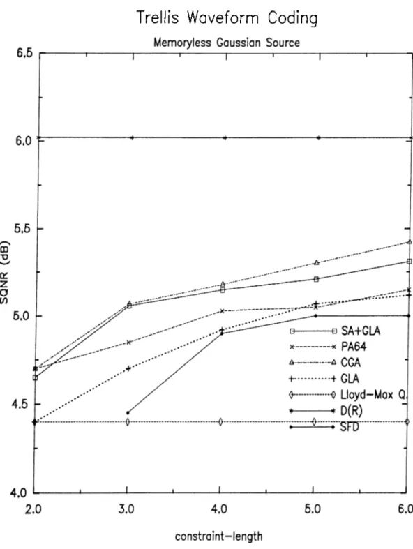
•5.1 Trellis waveform coder, SQNR results for Gaussian i.i.d. source, SA+GLA: Trellis waveform coder with simulated annealing and generalized Lloyd cilgorithm, PA64: Powell’s 1964 algorithm, CGA: conjugate gradient algorithm, SFD: Linde and. Gray’s scrambling function decoder, GLA: generalized Lloyd algorithm. 47 5.2 Trellis waveform coder, SQNR results for first order Gauss-

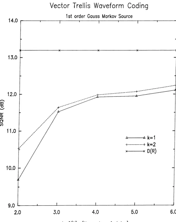
Markov source, SA+GLA: Simulated Annealing and General­ ized Lloyd Algorithm, GLA: Generalized Lloyd Algorithm only. 50 5.3 Vectoral TVVC vs scalar TWC, hrst order Gauss-Markov source 53 5.4 Finite-state vector (luantization, SQNR results for first order

Gauss-Markov source, 8 state trellis, SA+GLA : FSVQ with simulated annealing and generalized Lloyd algorithm, VQ: mem­ oryless vector quantizer, OLT+GLA : FSVQ with omniscient labeled transition ilesign method and generalized Llod algorithm. 56

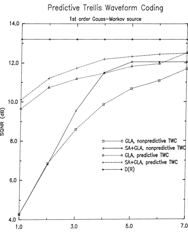
5.5 Predictive trellis waveform coder, SQNR results for first order Gauss-Markov source... 58 5.6 Predictive trellis waveform coder, SQNR results for speech

model source... 60 5.7 Ungerboeck trellises satisfying the branch labeling rules of

5.1 SQNR [dB] results for the memoryless Gaussian source. K: con­ straint length, SA-I-GLA; trellis waveform coder with simulated annealing and generalized Lloyd algorithm, PA64: Powell’s 1964 algorithm, CGA: conjugate gradient algorithm, .SFD: Linde and Gray’s scrambling function decoder, GLA: generalized Lloyd al­ gorithm ... 46 5.2 SQNR [dB] results for the first order Gauss-Markov source. K\

constraint length, SA-fiGLA: simulated annealing iuid general­ ized Lloyd algorithm, GLA: generalized Lloyd algorithm only.

5.5

51 5.3 SQNR [dB] results for the first order Gauss-Markov source with

different truncation depths. K: constraint length, TD: trunca­ tion depth... 51 5.4 SQNR [dB] results for scalar and vector trellis waveform, coding

where the systems with k — \ and k = 2 are designed using SA-f-GLA and results for k = 3 and k = 4 are those of the labeled state vector trellis encoding system. N: number of states, k\ vector length, LSVTE: labeled state vector trellis encoding system. 54 SQNR [dB] results for 8-state FSVQ and VQ for the first order Gauss-Markov source, k: vector length, SA-I-GLA : FSVQ with simulated annealing and generalized Lloyd algorithm, VQ: mem­ oryless vector quantizer, OLT : FSVQ with omniscient labeled

transition design method. 55

5.6 SQNR [dB] results for the first order Gauss-Markov source. K\ constraint length, SA-f-GLA: simulated annealing and general­ ized Lloyd algorithm, GLA: generalized Lloyd algorithm only. 57

5.7 SQNR [clB] results for the speech model source, /v: constraint length, SA+GLA; simulated annealing and generalized Lloyd algorithm, (JGA: Powell’s conjugate gradient algorithm, GLA:

generalized Lloyd algorithm only... 61

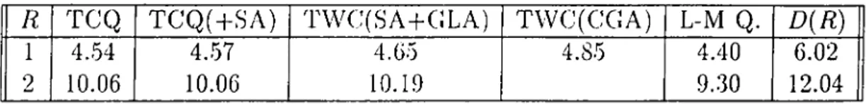
5.8 Comparison of trellis coders for Gaussian i.i.d. source, = 4, L-M Q.: Lloyd-L-Max quantizer, CGA: Conjugate gradient algorithm 62 5.9 = 4, first order Gauss-Markov source, a = 0 . 9 ... 64

5.10 Predictive trellis coding results for first order Gauss-Markov source 64 5.11 Predictive trellis coding results for speech model s o u r c e ... 64

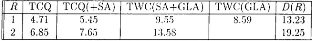
5.12 7? = 1, performance comparison of possible branch labelings for Ungerboeck trellis, Gauss-Markov sources... 67

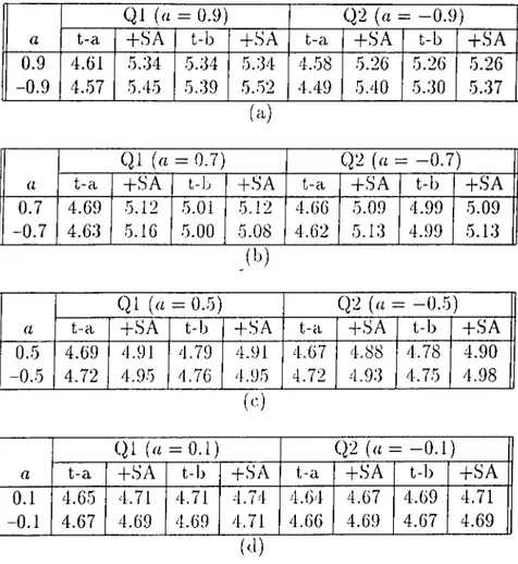
5.13 Trellis-a and trellis-b comparison (t-a: trellis-a, t-b: trellis-b), -fSA: performance with SA on the trellis the SQNR of which is given in the previous column, Ql and Q2 denote the quantizers with Lloyd-Max output points calculated for SI (source 1) and S2 (source 2) respectively. Source 2 has a correlation coefficient that is negative of Source I ’s. 68 A.l K = 2, TWC, Gaussian i.i.d. so u rce... 75

A.2 K = 3, TWC, Gaussian i.i.d. so u rce... 75

A.3 K — 4, TWC, Gaussian i.i.d. so u rce... 76

A.4 K = 5, TWC, Gaussian i.i.d. so u rce... 77

A.5 K = 6, TWC, Gaussian i.i.d. so u rce... 78

A.5 K = 6, TWC, Gaussian i.i.d. so u rce... 79

A.6 K = 3, TWC, first order Gauss-Markov s o u rc e ... 80

A.7 K = 4, TWC, first order Gauss-Markov s o u rc e ... 81

A.9 K = 6, TWC, first order Gauss-Markov source ₈₃

A.9 K = 6, TWC, first order Caiiss-Markov s o u rc e ... 84

A .10 K = 7, TWC, first order Gauss-Markov source 85 A .10 K = 7, TWC, fii'st order Gauss-Markov source ₈₆ A. 10 K = 7, TWC, first order Gauss-Markov source 87 A .10 K = 7, TWC, first order Gauss-Mcirkov Source 88 B.l N=4, VTWC, first order Gauss-Markov source 90 B.l N=8, VTWC, first order Gauss-Markov source 91 B.2 N=16, VTWC, first order Gauss-Markov source 92 B.2 N=16, VTWC, first order Gauss-Markov source 93 B.2 N=16, VTWC, first order Gauss-Markov s o u r c e ... 94

C.l k = I, N = 8., FSVQ, first order Gauss-Markov source 96 C.2 k = 2, yV = 8, FSVQ, first order Gauss-Markov source 97 C.2 k = 2, N = 8, FSVQ, first order Gauss-Markov source 98 C.3 k = 8, N = S, FSVQ, first order Gauss-Markov source 99 C.3 k = 3, N = 8, FSVQ, first order Cfauss-Markov source 100 C.3 k = 3, N = 8, FSVQ, first order Gauss-Markov source 101 C.4 k = 4, yV = 8, FSVQ, first order Gauss-Markov so u rc e ... 102

C.4 k = 4, N = 8, FSVQ, first order Gauss-Markov so u rc e ...103

C.4 k = 4, yV = 8, FSVQ, first order Gauss-Markov so u rc e ...104

C.4 k = 4, N = 8, FSVQ, first order (Jauss-Markov .source... 105 C.4 k = 4, yV = 8, FSVQ, first order Cfauss-Markov source 106

D.2 K = 3, PTWC, first order Gauss-Markov s o u r c e ... 108

D.3 K = 4, PTWC, first order Gauss-Markov s o u r c e ...109

D.4 K = 5, PTWC, first order Gauss-Markov s o u r c e ...110

D.5 K = 6, PTWC, first order Gauss-Markov s o u r c e ...I l l D.5 K = 6, PTWC, first order Gauss-Markov s o u r c e ... 112

D.6 K = 7, PTWC, first order Gauss-Markov s o u r c e ... 113

D.6 K = 7, PTWC, first order Gauss-Markov s o u r c e ... 114

D.6 K=7, PTWC, first order Gauss-Markov s o u rc e ...115

D.6 K=7, PTWC, first order Gauss-Markov s o u rc e ...116

D.7 K = 2, PTWC, speech model source ... 117

D.8 K=3, PTWC, speech model s o u r c e ... 118

D.9 K=4, PTWC, speech model s o u r c e ... 119

D.IO K=5, PTWC, speech model s o u r c e ... 120

IN T R O D U C T IO N

The goal of design of any communication system is to build a system which enables the transfer of information-bearing signals from the transm itter to the receiver reliably, that is with “little” or no loss in information. To reach the goal of reliable communication, the information to be transm itted should be converted into a form that is in some way more “convenient” to transmit and then be converted back to the original form after transmission. Let the information source be in the form of a random process A^„. Then, a simple, yet general model of a communication system aiming a reliable transfer of information is as given in Figure 1.1.

A communication system is composed of three parts, an encoder, the chan­ nel, and a decoder. The channel represents the medium through which infor­ mation will be sent. The information which is represented by the input random jjrocess X,i is converted by the encoder into another random process Un which is more convenient to handle aiul to transmit over the channel. This process (Jn is sent through the channel, and at the other end of the channel another random process Un is received lyy the receiver which is related to Un through a conditional probability distribution. Then, the decoder performs the reverse

A X.

of communication system design is to minimize the difference between the input sequence, and X^^ the rej^roduction sequence.

Usually the channel puts severe restrictions on the type and the quantity of signals that can be transmitted through it. For example, most of the time one has to represent an infinite collection of input signals X ^ with a finite collection of signals Un· This introduces quantization errors into the commu­ nication process, causing a loss in information since there is no way one can recover Xn from Un- Other than this, the difference between X,i and Xn iTiay be due to some disturbances in the channel which corrupt the signal. These disturbances may be deterministic such as filtering, modulation, aliasing, or random such as additive noise, fading, and jamming. Then, the fundamental issues in communication system design are source coding or data compression which is the mapping of the input sequence (information source) efficiently into a representation for transmission over the channel and channel coding or error-control coding for overcoming the noise in the channel.

Claude Shannon formulated both of these issues in his classical papers [1], [2]. One important fact he proved was that in a communication system design, source coding and (nror-control coding (channel coding) can be considered independently: one can design seperate systems for source and channel coding and then simply cascade them. The result would be as good as the result of designing both systems together at the same time.

In our work, we focused on the problem of data compression, making some assumptions about the channel and then ignoring it completely, the approach being justified with Shannon’s above mentioned theorem. Our first assumption about the channel is that it is digital, that its permissible inputs and outputs form a finite set or alphabet. Our second assumption is that the rate of the channel is fixed, that is, for each channel input symbol chosen from the input alphabet there is just one output symbol f/„. The third assumption is that the channel is noiseless, that is =

Un-Data compression involves the design of the encoder and the decoder. As stated above, the encoder is a mapi)ing from the input sequence Xn into i/„, the channel input secpience. This ma,pping can be performed in many ways, the objective still being to minimize the difference between the reproduction

ular type of data compression is called qxLantization. Shannon’s distortion rate theory formulates the lowest distortion achievable for a given fixed rate with such a system but it makes no suggestions for the ways of actually building systems with optimal performance. Therefore, many researchers since Shannon have concentrated on finding the rules for the design of systems with perfor­ mance approaching theoretical bounds. Although many good coding systems have been suggested, there is still room before the bounds are reached. The goal of this work is to contribute to these efforts in the fields of trellis waveform coding and related systems using a different design approach.

Before we go into the details of our coding approach, we provide some background information on some important quantization techniques related to our work in the next chapter.

Q U A N T IZ A T IO N

T E C H N IQ U E S

2.1

Scalar Q u a n tiza tio n

Scalar quantization is the simplest of qucintization techniques. It is simple because it performs quantization on a discrete time sequence considering the samples one by one, in other words, it quantizes the samples independently. The scalar quantizer is defined with a codebook C = {yi, J/2, · · - yN) composed

of the codewords ?/,s which iire the reproduction values, and an encoding rule, which determines the way in])ut symbols are encoded to one of r/,s. The code­ words partition the input space into N regions, ,S'i, .$2) · · · > <5'^/·, each Si being

composed of the points in the s])ace that are assigned to ?y,· through the en­ coding rule. The elements Xn from the input sequence {.ri, ;r2, . . . , x’l} are

quantized one by oiuj according to the encoding rule, that is, a symbol from the input sequence is quantized to ;iy, if it falls into the region .5',·. An impor­ tant special case of the ciuantizer is the Nearest Neighbor (NN) quantizer. In NN encoding, the distance of :;;,i from each yi is calculated via the distortion measure d{x,i, yi) and Xn is quantized in the following way.

— yji 11 Si yi)i Vi G {1,2, .. . N }i (2.1)

where q(x) denotes the (piantizer function. If the equality holds, that is, if there is more than one such j , the choice is maile randomly. The encoder being the NN encoding rule, the decoder is simply a look-up table (the codebook itself)

rule and a codebook which gives the best performance for input in terms of a performance criterion, over all possible encoding rules and codebooks. The dif­ ference between the input seciuence and the reproduction sequence is referred to as distortion. In order to measure the “distance” between the source sequence and the sequence of the quantized samples, one uses a mesaure, known as the distortion measure, between the two sequences. A wide class of distortion mea­ sures are known as per-letter distortion measures, i.e., the contribution from individual samples and their quantized values in a sequence have independent effects; for example, for additive distortion measures, these contributions are additive. There are various functions proposed in the literature as measures of sample distortion.

The most common (.listortion measure between two vectors x and x whose members are .t, and ;t·,, 0 < ?’ < A: — 1, is the squared error distortion or the square of the Euclidean distance:

k - \

d(x,x) = I ^ I

(

.

)

¿=0

Other possible distortion measures are Holder iiorm.

A.—1 Minkowski norm^ </(x,x) = I Xi - Xi I"} t=0 d (x ,x ) = max | .c,· — .i·,· |, 0<г<^·—1

and the weighted-squares distortion^ A—1 d(x ,x ) = W{ I X{ I , (2.3) (2.4) (2.5) ¿=0 where in,· > 0, i = 0 , . . . , A' — 1.

These distortion measures are called (.lilference distortion measures since they depend on the vectors x and x oidy through the difference vector x — x. Other types of distortion measures are also used in tlata com])ression systems but they are more complicated. Throughout this thesis we will only use the squared error distortion measure l)ecause it is commonly used in the data compression literature and because of its mathematical tractability.

A direct generalization of scalar quantization (SQ) to higher dimensions, that is, coding of symbols in blocks with length more than one is vector quantization (VQ). A vector quantizer Q of dimension k and size is a mapping from a vector in the ¿-dimensional Euclidean space 7?.^’ into a finite set C containing N codewords or reproduction ])oints. That is.

Q : K ‘ ->C, C = {yi,y2.---,yw) Mid y, €

(

.

)

W ith analogy to the scalar case, the codewords y,s in the codebook C partition the input vector space into N regions each composed of points in the space which are associated with y,·. Each vector x,i from the input sequence is encoded into y,· only if it is in Si. Again, a special case is nearest neighbor encoding where the quantizer computes the distortion between the input vector and each codevector in the codebook and encodes the input vector to the one which gives the smallest distortion. That is,

Q M = Yj if <K^n,yj) < (l{^n,yi), 3 j ,V i e (2.7) where, again the choice is made randomly if the equality holds.

Vector quantization is more efficient than scalar quantization because it can exploit the correlation lietween samples which SQ cannot do since it quantizes the samples independently. Moreover, even if there is no statistical correlation to be exploited between the siunples, VQ can do better than SQ due to its higher freedom in choosing decision regions for jiartitioning [4].

Since the quantizer is completely S])ecified by a codebook and an encoding rule, the design objective of vector quantizer is to find a codebook corre­ sponding to the decoder and an encoding rule corresponding to the encoder, that will give the best performance. For a given codebook C, the average distortion (for empirical data) can l)e lower l.)ounded according to

(2.8)

A. = l

-This lower bound is achieved if Q assigns each vector Xf. in the input sequence to a codeword which is the nearest neighbor condition. Looking for the optimal codebook given the partition h'ads us to the centroid condition. A centroid.

:.'ent(5) = m iir'E (d (X ,y ) | X G 5) (2.9) where the inverse minimum notation means the vector y satisfying the mini­ mum is chosen.

It is easy to show that for the squared error distortion measure, this leads to the center of mass of S. For empirical data, the center of mass of S is.

cent (5) = 1 S

Ill’ll 1=1

(

2

10

where the summation is over the vectors x,· that are in S. Then, given the partition (or equally the encoding rule) the oj)timum codebook is composed of the center of masses of each partition cell.

These necessary conditions of optimality suggest an iterative means of nu­ merically designing a good vector quantizer. Given S one can start with an arbitrary initial codebook and partition S according to NN. Then the optimal codebook for this partition is found I:>y computing the centroids and the new partition can be found for the new codebook. Iteratively, this procedure pro­ ceeds to better codebooks. This algorithm is known as the Generalized Lloyd Algorithm (GLA) or the LBG algorithm [3]. Although there are various vector quantizer design methods [4], GLA is the most popular and several extensions of it are made in the literature. The extension that is of interest to us is the one intoduced by Stewart et al. in [20] in the context of trellis waveform coding which we will discuss in length in the coming sections. At this point we give GLA in its original form as was introduced by Linde et al. [3] for VQ:

The Generalized Lloyd Algorithm

1. Begin with an initial codebook Go. Set m = 0, and a threshold value e > 0. 2. Given the codebook. Cm = {yi},

partition the training set into cells ,S', using the NN condition: Si = {x : d(x,y,·) < d (x ,y j); Vj / /:}.

3. Compute the centroids of the partition cells. Si using (2.10), update the codebook according to the centroid condition: Cm+i = {cent(,S;·)}.

stop with codebook An+i, else, set m <— m + 1.

2.3

F in ite -S ta te V ector Q u a n tiza tio n

Vector quantization, as discussed in the previous section, considers each vector independently and therefore does not take into account the future or past vectors. Therefore the right term to define standard VQ is memoryless VQ.

As discussed in the previous section, the superiority of VQ to SQ (scalar quantization) partly comes from the fact that VQ exploits the correlation among the samples in the block. And the bigger the vector (or block) di­ mension is, the more VQ will exploit the statistical dependences in the se­ quence, since it will see more samples at a time. At this point, it is clear that contending with a finite vector size and quantizing the blocks seperately, we are ignoring the dependencies Ijetween samples in consequetive blocks which could be exploited for even better coding performance. One apparent solu­ tion to this problem is to increase the vector dimension indefinitely which is then accompanied with a pro])ortional increase in computational complexity, which becomes unmanagable. Since this solution is not practical, instead of introducing more sam])les in the quantization process, we should include the information about these samples to the current quantization instant in some way, that is we should introduce memory into the quantizer. This memory is used to derive information about statistical dependencies between samples, and this information is ex])loited for better coding performance. This can be realized in the following manner.

In standard (memoryless) V(), we base our quantization decisions on a fixed codebook C = { y i,y2) · · · lyAf}· Instead, we think of employing a codebook

changing with time, we let a dilferent codebook be used at each quantization instant and choose this codel)ook from a. collection of codebooks according to the output of the previous ([uantization instant. Using the knowledge of

designed to suit different characteristics typical of the source, and the codebook selection procedure is designed properly as a good predictor of the trajectory the source will follow, interblock correlations will be exploited and the perfor­ mance will increase. This form of vector quantization is called recursive vector quantization [4]. The important special case of recursive vector quantization is when the collection of codebooks contains only a finite number of codebooks and this VQ is called finite-state vector quantization (FSVQ) [4]. Choosing a different codebook from a finite collection of codebooks at each quantization instant suggests a “state-based structure,” where each state is identified with the choice of codewords composing a particular codebook. The state with the codebook associated to it, which we can name as the state-codebook, describes the mode the quantizer is in, and is in a way a summary of the past behavior of the source. This “state-based structure” is a finite-state machine specified by a next-state function, determining state transitions and a decoder mapping which decodes the input bit stream to a re])roduction symbol (a codeword from the current-state codebook).

The best way to pictorially describe the F.SVQ finite state machine is through an example state transition diagram shown in Figure 2.1 with the assumption that the rate of the system is one bit per sample, corresponding to binary transitions or state-codebooks with size two. This FSVQ has four states, represented by circles numbered as 00, 01, 10, and 11. The lines with arrows represent possible state transitions at a decoding instant. y,jS are code­ words from the ith state-codebook. For instance, the channel symbol 0 when the quantizer is at state 01 i>roduces a reproduction symbol yio, the codeword from state codebook 1 with index 0, and causes the quantizer to move to state 10. The transitions are equivalent to the next-state function, the labels of transition lines with the states are equivalent to the decoder mapping.

Now, let us give a formal definition of the finite-state vector quantizer (FSVQ):

Define a state space S as a collection of .symbols S = {.Sj, .S2, . . . , ¿'/c-i}

called states. Let the vector dimension lie k. Let the set of channel symbols be U = {uo, U i,. . . , U/v-i}. The coding rate is log/V bits per input vector or log iV bits |)er source symbol. Then, a finite-state encoder is a mapping cv : X S —y U, that is, given an iii])ut vector x and the current state s

the function o:(x, .s) maps x into u, a channel symbol. In addition to the encoder mapping, the quantizer is defined by the next-state mapping which is the essential difference of FSVQ from other VQ techniques. The next-state mapping is a function / : ¿Y x <S —> <S which produces the next state / ( u ,s ) , given the current state s and an output symbol u produced from the input symbol X .

Correspondingly, a finite-state decoder is a mapping fi : U x S —>■ 7^^’, that is, given the current state s and the channel symbol u it produces the reproduction symbol x.

The output spaces of the encoder and decoder mappings are required to be the same, also the next-state mapping is resctricted to depend only on the current state and the encoder output rather than the input symbol. These two restrictions enable the encoder to track the state sequence given the initial state, and one does not need to send the state information in addition to the channel symbols.

To each state, .s, a fitatc codebook, C, = {/7(u, .s), u G ¿/}, is associated which is composed of the possible reproduction vectors in that state.

Then, the encoding process of a random process {A^,,n = 0 ,1 ,2 ,...} can be described as follows. Given an initial state sq G <5, the channel symbol sequence, the state sequence, and the reproduction sequence are produced re­ cursively for n = 0 ,1 ,2 ,... as:

u „ = cv(x„, 6 ;) .sw, = / ( u , „ Sn) Xn = Sn). (2.11)

To complete the definition of FSVQ, we should also specify the encoding rule: FSVQ encodes according to minimum distortion or nearest neighbor condition. That is, using the Euclidean distance as the distortion measure, the encoder mapping a is defined by

«(x, .s) = min ‘d(x,/:l(u, .s)) (

2

12

which means that a(x , .s) is the index u for which the reproduction codeword )il(u,s) yields the minimum possible distortion over all possible reproduction codewords in the state codebook Cs- In our discussion on vector quantization we noted that the minimum distortion encoding rule was the optimal encoding for a given codebook. Although in FSVQ minimum distortion encoding seems the most natural choice, in the long term, it may not be the best choice. Because, FSVQ with minimum distortion encoding optimizes only the short term performance of the system. Because of the memory in the quantizer, a codeword with very small distortion can lead to a state with a bad codebook for the next input vector. But, the minimum distortion rule is intuitively satisfying and no better encoder structure with comparable complexity is found so far. Therefore, we will contend with this encoding rule.

Suboptimality of the minimum distortion encoding in FSVQ is the conse­ quence of FSVQ’s having a memory of only one vector size. The remedy is to have an encoder with a memory of iii])ut sequence size which leads us to the trellis encoding system that will be discussed in the next section.

Note that VQ is a special case of FSVQ with only one state. Although FSVQ is more general, distortion ixite functions of information theory show that, optimal achievable ])erformance (average distortion) for a given rate is the same for both cases [5]. But the performances of FSVQ and VQ are the same only when arbitrarily large vector dimensions are allowed. FSVQ, because of its higher ability to exploit correlations between samples, obtains the same performance with VQ using shorter vectors, therefore it provides systems with lower complexity.

Based on the finite-state machine perspective, we can identify two different ways of relating the state sec|uence and the reproduction sequence. These are pairing of each reproduction vector with a state or with a transition. The first type of FSVQ is called labeled-state FSVQ and the second one is called labeled-transition FSVQ.

The decoder mapping /i of a labeled-state FSVQ depends on the current state and channel symbol only through the induced next state; the current reproduction Xn is determined by the next state Sn-i-i· On the other hand, the decoder output of a labeled-transition FSVQ is associated with the tran­ sition from the current state to the next state and therefore is determined by both the current state and the next state s,i+i. These two configurations correspond to two different finite-state machines: labeled-state FSVQ to the Moore machine.! labeled-transition FSVQ to the Mealy machine [7]. The two structures are equivalent in the sense that Mealy and Moore machines are equivalent [6]. That is, given one, one can find an equivalent FSVQ of the other form, equivalent in the sense that given an initial state and an input sequence, the two quantizers will yield the same output sequence. The code­ words are held constant in transition from one form to the other. For example, going from labeled-transition FSVQ to labeled-state FSVQ the codewords that were assigned to branches are assigned to separcite states which amounts to an increase in the number of states.

As noted above, an FSVQ is fully determined by an encoding rule, state codebooks and the next-state function. Therefore, the design of a FSVQ fo­ cuses on generating state codebooks and a next-state function. First, we con­ sider finding a good encoder a and a good decoder /i given a fixed next-state function / . Finding the best decoder for the given next-state function and given encoder is equivalent to finding the best state codebooks. Suppose we have an input .sequence {X„; = 1 ,2 ,..., L}. If the initial state is .Sq, encod­ ing, we obtain the channel .symbols U,i = (v(X,i,.s,i) and the state sequence

= /(U ,i,s,i) for n — 1,2, . . . , L . Then our goal is to find the decoder mapping (d minimizing the distortion,

D = l x ; , i ( X , „ / i ( U , (2. 13) ^ n=l

It is easy to show that optimal decoder cod(wectors are the centroids [4], that

IS,

/^(u,.s) = min ' ■ -/— -T, .

I I I I

^

rf(x...y)

where M (u, s) is the collection of U„ such that Un = u.

This is the optimum decoder for the given encoder and the next-state func­ tion, but the encoder may not be the optimum one for the obtained decoder, so the next step is to find the optimum encoder for the given decoder. Now we perform a nearest neighbor encoding using the state codebooks found and the given next-state function, which yields a new partition and therefore a new encoder a. Then, we should find the best decoder for the current encoder and given next-state function and the process of finding the best encoder and de­ coder continues iteratively until no significant performance gain is obtained by subsequent iterations. This procedure is indeed a variation of the generalized Lloyd algorithm. We can summarize the algorithm as follows.

FS V Q E n c o d e r/D e c o d e r D esign A lg o rith m 1. Initialization:

Given: a state space <S, an initial state Sq,

an encoder ao

a next-state function / ,

a training sequence {Xn; n = 1 ,2 ,..., L}. Set e > (J, m = l. Do = oo.

2. Encode X„, n = 1 ,2 ,..., L, using a,n-i to obtain {U„, s„}; n = 1 ,2 ,..., L.

The state codebooks are modified into ^ ( u , s ) = cent(u,s).

3. Replace the encoder by the minimum distortion encoder am for ^m-Compute the distortion Dm·, if l^m — Dm-i\IDm < e quit else goto stepl.

Then, the problem left is to design the next-state function. Several methods are proposed in the literature to solve this problem. These methods include Conditional Histogram Design, Nearest Neighbor Design, Set Partitioning, Om­ niscient Design, etc. A detailed discussion of these methods can be found in [4].

Conditional histogram design is one of the simplest techniques. First, the algorithm forms a supercodebook through applying GLA with standard VQ. A state is assigned to each codeword thus found. Then the method estimates the conditional probabilities of successor codewords in the supercodebook which is

named the classifier codebook und forms a labeled-state FSVQ by only including the most probable codeword successors in the classifier codebook to the state codebook. Since the codewords are assigned to states, the choice of state codebooks also determines the next-state function.

The method called nearest neighbor design also generates a classifier code­ book in the same way, but uses the distortion between the codewords and not the conditional probabilities for selecting the set of allowed new states from a given prior state. For each state assigned to each codeword in the classifier codebook, N nearest neighbors are found and the state codebook is formed with these codewords. Hence the next-state function is formed.

Another FSVQ design techniciue, called omniscient design was introduced by Foster et al. [7] and Haoui and Messerschmitt [8], and developed for speech coding by Dunham and Ciray [9] and for image coding by Gersho and Aravind [10]. This method is more complicated than nearest neighbor and conditional histogram methods but it usually shows better performance and it can be used with more general classifiers than VQ. Although nearest neighbor and conditional histogram techniques are for the labeled-state FSVQ design, the omniscient method can be used for both labeled-transition and labeled-state FSVQ design. The details of this algorithm can be found in [4] and [7]. Ref­ erence [7] also provides simulation results for the comparison of various FSVQ design techniques. These results show that omniscient labeled-transition design (OLT) gives the best results for sources of practical interest. This method is also referred to in [4] as the method through which best results are obtained thus far.

One of the contributions of this work is to suggest and show a design algo­ rithm that has better performance than the methods described above, which will be described in Chapters .'3-5.

2.4

T rellis W aveform C od in g

In this section, we turn our attention to a more advanced data compression scheme, trellis utaveform coding^ which is the main qucintization scheme on which our work has focused with the goal of designing a near-optimum decoder.

early 1980s, who made considerable progress towards an understanding of trellis encoding systems. The popularity of this data compression system is partly due to the fact that results in information theory have proved the existence of trellis systems which show performance close to the theoretical bounds [11], [12]. But these are only existence proofs, which do not describe the actual ways of constructing good codes. Therefore many researchers concentrated on the problem of finding rules for constructing good codes and came up with various design algorithms. The goal of this thesis is to make a contribution to these efforts, which has been achieved by designing an algorithm for constructing near-optimum codes based on an ajjproach different from other work in the literature.

We will now describe the trellis waveform coding system. In the previous section, we discussed a VQ system called FSVQ. As was noted, FSVQ is supe­ rior to VQ due to the incori)oration of memory into the quantization process. But as also explained, minimum distortion encoding may not be optimal in FSVQ, since a codeword with very small distortion can lead to a state with a bad codebook for the next input vector. Although through good design one can try to eliminate this problem, we can never be sure about the optimality of the encoding.

This observation leads us to tlie conclusion that the suboptimality of FSVQ encoding is due to its having a memory size of only one vector and the remedy is to increase the memory of the FSVCJ encoder from vector size one to vector size M\ instead of making “greedy” ciuantization decisions on vectors one by one, to delay the decision until M vectors are seen and to decide on these M vectors together. Then the quantizer will make a decision which is good for at least M vectors, and the jn'obability of making bad decisions will decrease. In this manner, we expect to have an optimal encoder as M approaches the length of the vector sequence.

This operation is called delayed decision encoding^ lookahead encoding, mul­ tipath search encoding, or trellis encoding, for reasons that will become appar­ ent. For delayed decision encoding, we employ a finite-state machine for the decoder as in FSVQ where the states summarize the past behavior of the sys­ tem, and approximate the current mode of behavior of the input sequence. In this case, the forms of encoding, decoding, and next-state mappings are differ­ ent. In FSVQ, the state transition diagram (finite-state machine) is sufficient to explain the operation of the .system; but in delayed decision coding, we need

a more elaborate structure tliat takes the past into account explicitly.

For convenience we repeat here Figure 2.1 as Figure 2.2.a, which shows the state transition diagram of a FSVQ. The extension in time of the state transition diagram is the directed graph given in Figure 2.2.b. The stages in the graph corres])ond to consecutive time instants of the data compression process and each stage is ccpiivalent to the state transition diagram. Each node corresponds to a distinct state at a given time, and each branch originating from a node represents a transition from that state (node) to some state (the node which the branch is connected to) at the next instant. The graph begins at state 5o and ends at To each branch in the graph certain weights are assigned which are the reproduction symbols-or state codewords- in the FSVQ state transition diagram. This directed graph is called a trellis and it is a special case of a i/’ce, branches of which are self-emerging, that is, branches originating from a common root (node) can meet again at another node later in the tree. The encoding system b£ised on this data structure is called the trellis source coding system. To every possible state sequence of the trellis there corresponds a unique path. Given the channel symbols, the trellis can keep track of the state sequence and generate the reproduction symbols out of the state codebooks.

The trellis structure thus described can be used to represent a vector quan­ tizer if the trellis has only one state or a finite-state vector quantizer but to represent a trellis encoding system we introduce measures assigned to each node along the trellis. The measure assigned to a particular node corresponds to the total distortion of a state sequence that starts at state .Sq and ends at that node.

The encoder performs a nearest neighbor encoding in the following manner. At each time instant, for each node, it considers the input branches to that node and computes the distortions due to the codewords corresponding to these branches. Summing the node-distortion of each node which these branches originate from and the calculated distance of the corresponding branch, the total distortion faced by a particular path is calculated. The encoder decides on the path with the least distortion and assigns the distortion corresponding to this path to the node under consideration; it also stores the index of the branch connected to that node. Therefore, the encoder is a trellis search al­ gorithm which tries to find the path with the minimum distortion. There are various algorithms in the literature for trellis search, Viterbi Algorithm (VA) [1.3] being the most popular one. Tlx; reason for its popularity is that it is an optimal search algorithm. A well-known alternative, the M-L algorithm, is not

STATE

к = о k=l к = 2 _У(Ю к = 3 к = 4 k = L-l k = L

optimum and it is better suited for tree search since it takes no advantage of the simpler trellis (self-emerging tree) structure.

The Viterbi algorithm was first suggested by Viterbi in 1967 [14]. It was later shown by Omura in 1969 [15] that it was a special case of dynamic pro­ gramming. Here we summarize this important algorithm.

2 .4 .1 V i t e r b i A l g o r i t h m

Given : a collection of states S = (Tq, <t i, . . . , ctm-i·, a starting state sq,

an input vector sequence :ri, x-2, . . . ,x l,

a decoder /i(n, .s).

Let d(.,.) denote the squared Euclidean distance and Dj{k) denote the total distortion for state k at time j.

1. Set Z)jt(O) = oo, 1 < A; < M 2. For 1 < n < L do

2.1 For 0 < k < M do

2.1.1 Calculate d(j,k) for all states j from which a branch to state k exists

2.1.2 Df,{n + 1) = m,in(Dj(n) + d(j, k))

J

2.1.3 Eliminate the branches other than the branch

achieving the minimum above. Save the optimum branch. 3. Find \mi\Dk{L) which is the minimum distortion obtainable.

Trace back the survivor i^ath, which is the optimum state sequence.

Although the Viterbi algorithm is very favorable due to its optimality, there is a price paid for this. First of all, coni])utational complexity is higher when compared with FSV(J. Second, there is the important practical problem that the algorithm does not make a decision on the o])timum ])ath until it reaches the final node. First of all, this amounts to the storage of all the survivor paths until the algorithm e.xecution is completed. One observation enables us to get around this difficulty: most of the time we .see that the survivor paths at time

k have a common root some / stages back at time k — 1. Then the survivor paths are said to have merged at deptli /. If all the survivor paths at time k have merged at depth /, we can safely make a decision about the optimum path up to time k — I without waiting until the end of the sequence. An efficient way of performing truncated search is to stop the normal execution of VA at certain instants periodically and perform a back search to find the root, where the survivor paths are merged. When the root is found, a decision can be made for the optimal path before the root and the cursor of the storage array is simply moved to the root. Even if we cannot find a root, considering the path with the lowest distortion up to the decision node, we can force a decision for the optimum path. If we keep the period of searches large enough, that is, if we keep the truncation depth large enough, the probability of making errors in the truncations will be low. In the literature [16], a truncation depth T D of 5 times the constraint length is suggested. Obviously, performing VA with truncated search greatly reduces the memory storage requirements. Instead of storing L X N integers we just store I'D x N integers and usually T D L.

Another reason for ])referring truncated search VA to standard VA is that when a coder is to be used in interactive applications, because of practical delay reasons, search lengths should be kept short. For typical interactive speech applications the practically allowable delay is no greater than 40 milliseconds which corresponds to search-length values around 256 in rate 1 bit/sam ple communication. But, of course, there are no such restrictions in broadcast or storage applications and as long as there is need to do so, long search lengths can be used.

Since the encoder of the trellis waveform coder is simply a trellis search algorithm for which we choose the Viterbi algorithm to use, the problem left is to design the decoder which is the objective of this thesis.

2.5

P r e d ic tiv e Trellis W aveform C od in g

Another way of incorporating memory into the quantization process is to in­ clude prediction to the encoder. In the literature, this approach was applied to vector quantization and gi-eat improvement over standard VQ was reported [4]. An interesting approach was reported later by Ayanoglu and Cray in [19] who replaced the VQ encoder with a trellis encoder and named the new system

predictive trellis waveform coding (PTWC).

Our knowledge of DPCM states that for a good predictive encoder, pre­ diction error samples are approximately white. Therefore, if the predictor is well-designed, combined with the advantages of trellis waveform coding, PTWC will exploit most of the redundancy in the source.

Predictive trellis waveform coding system is expected to perform better when compared to noiifeedback trellis encoders since whitening the source, which prediction does efficiently, means exploiting the statistical redundancy of a source better. It is also expected to perform better than DPCM due to delayed decision encoding for reasons explained before. One more advantage offered by delayed-decision encoding is the stabilizing effect on the decoder prediction filter [18].

2 .5 .1 S y s t e m D e s c r i p t i o n

The encoder and the decoder of the predictive trellis encoding system are as given in Figure 2.3. In the encoder, the output of the predictor which tries to approximate the input is subtracted from the input to obtain the error symbols {ejt}. Having the error symbols as input, the trellis search decides on the best choice of a channel symbol sequence {ziA,.} through minimum distortion encoding. Channel symbols ua’s are sent through the channel and received by

the decoder which converts them into codewords with corresponding indexes. The decoded codeword is then added to the predictor output which is the same as the predictor in the encoder. As in the case of DPCM, the reconstruction error Xk — Xk is equal to the (|uantization error e.k — (j{ek) = (xk — d:k) — {¿k — ¿k) where (j{ek) is the codeword assigned to e-k·

The most essential ])art of the system is the predictor, the design of which should be done carefully so that it predicts the input sequence efficiently. Ayanoglu and Gray used a linear time invariant predictor since this would keep the decoder complexity low and would enable the use of relatively simple design techniques leased on linear ])rediction theory [19].

U,

(a)

(b)

[19], we should specify the trellis search algorithm and the codebook and pre­ dictor design algorithm. The trellis search algorithm aims at the optimal min­ imum distortion encoding of the input sequence in the presence of a predictor. Due to the finite state machine structure, a trellis search algorithm is possible and it is a modified version of the Viterbi Algorithm.

2 .5 .2 S e a r c h A l g o r i t h m

The search algorithm should keep an estimate for the previous Lp reproduction symbols Xk-i along the survivor path leading to state j , which will be used by the predictor at time A; -f 1. Let Xk{j , l), l = l , . . . , L p represent Xk-i along the path leading to state j at time k. Let Xk{j) = { ^ k { j A ) T - - i ^ k { j ^ L p ) y ^ a = ( a i , . . . Let Di,{j) represent the total distortion associated with the j th node at time k. Let y{i,j) be the codeword on the branch connecting nodes i and j . The predictor order is Lp.

0. Initialization: Do{0) = 0, Do{j) = oo, 1 < i < - 1, X o ( i) = 0, 0 < i < 2^ ' - * - l , 1. Recursion: For 0 < k < Lb — U do 1.1 For 0 < J < 2^'“ ’, do

1.1.1. Dynammic programming step:

Dk+i{j) = mini{Dk{i) -I- (l(xk,a^Xk{i) + y{i,j)))·

The index i is from the set of all nodes from which a path exists to node j. Save the argument minimizing this equation as Ik(j)·

1.1.2. Update the first element of Xk{j) íis Xk+iU, 1) = a^Xki hU) ) + y { I k U) J ) 1.1.3. Prediction update:

Xk+x{jJ) = X k { I k { j ) . l - 1), 2 < / < Lp.

2. When ii = L — 1, find j such that = m inD /,_i(j). i

Release the corresponding pathmaj) through the trellis to the channel.

The search algorithm is a direct extension of Viterbi algorithm and reduces to it for a = 0.

2 .5 .3 D e s i g n A l g o r i t h m

The encoder is specified by two sets of parameters: the linear prediction coefficients, a,·; f and the prediction error (residual) codewords, yk', k = 0 , . . . , 2 ^ — 1. The performance of the coding system is totally depen­ dent on the good design of these parameters. The design algorithm assumes initial values for these parameters and then iteratively improves them. The initial values for the codewords can be generated with any of the known meth­ ods particularly with extension [20] or splitting [3]. The natural choice for the initial predictor coefficients is the solution of the VViener-Hopf equation, R a = V, where R = ‘'-»d v = This choice for the initial pre­ dictor coefficients is based on the assumption that the original source inputs rather that the reproductions are the observables. We use coded reproduc­ tions in the predictive system therefore these parameters are not optimal, but these choices are intuitive and are good starting points for the design algorithm which improves them iteratively.

For a fixed prediction vector a, the distortion for the given training source

IS

Y(^d{xn,Xn) = - X n f = - Cnf.

71=1 n=l 71=1

(2.15) This distortion is minimized if we change the codewords into centroids of par­ titioning cells,

= (2.16)

II II71G.S·

We try to ]n*eclict Xy^ by

Xyi — ^ —

/=1

(2.17) The orthogonality ])rinciple [4] implies that a should be such that the prediction errors and the observations are orthogonal. This leads to

L - \

^ ^ (■C'?i •Cn)-l'n—i — fi) ^ — 1) · · · ) kp.

ii=0

Substituting

(2.18)

j= l *:=I A.'=l

Now, we state tlie predictive trellis wavelonn coder design algorithm. 0. Initialization:

Generate initial codebook Co = ij'f·, i = () ,..., 2”‘“ '

Find initial predictor c|ueiiici('iits solving the Wiener-Hopf equation, R a where R = and v = [/i’,]L,,xi·

1. Trellis Codebook U])date:

Encode the training sequence using and

L

in order to obtain Z)'“ = A:=l

If < i stop with

Vi = 0 < < 2^'“ ’ and (li — «■", 1 < i < L,,,

else update the trellis codebook according to (2.16) to ol>tain 2. Predictor Ui)date;

Use {2/,·"'*’^} and {u·“) to encode tlie training sequence.

Use (2.20) to obtain the new generation of ])redictor coefficients 3. Set m <— m + 1, go to 1.

= V,

2.6

T rellis C od ed Q u an tization

Another data compression system based on trellis encoding and finite-state machine decoder is the trellis coded quantization (TCQ). This recently intro­ duced data coiTi])ression system is rei)orted to give good results for memoryless sources and in predictive trellis coding [4].

Trellis coded quantization was first introduced by Marcellin and Fischer [51], who, motivated by the success of trellis coded rnodulation (TCM) in the field of modulation theory, and the results of alphabet-constrained rate distor­ tion theory, constructed the source coding analog of TCM.

In 1982, Ungerboeck formulated coded modulation using trellis coding and introduced the ideas of set partitioning and branch labeling for trellis coder

are most resistant to noise induced errors if tliey are very diil’erent from each other, that is, if th(u*e is a. larg(‘ distaiic(‘ in Euclidean signal space between the signal sequences. Following this fact, TC'M do'signs the signal map])ing function so as to nuiximize dir('ctly the '1Ve(' distance” (minimum Euclidean distance) between coded signal se(|uences. ('oinl)ined with the use of signal-set expansion to provide redundancy for coding and use of a finite-state encoder, this method led to a modulation scheme su]>erior to conventional modulation techniques.

A particular TC'M system is s])ecilied l)V the trellis structure (next-state function) and the codes assigned to trellis branches. As for the trellis struc­ tures, Ungerl)oeck suggested some symmetric trellises for N = 4 and N = S states. The branch connections are similar to the ty]ucal trellis of Figure 2.2 but for rates higher than 2, the transitions are multiple, that is each branch on the graph corres])onds to 2 or more |)arallel transitions. On a conventional modulation system for a signal constellation of size 2”^ in bit codes are used to send one of the 2”^ symbols. In trellis coded quantization, the signal constella­ tion is first doubled to ])oints. Then this constellation is ])artitioned into

subsets, where ih is an integer less than or equal to in. ih of the inj)ut bits are used to select, by trellis encoding, which of the subsets the channel symbol for the current signaling instant will be chosen from. The remaining 771 — 77A bits are used to select one of the channel symliols in the selected subset. By this way although the rate of the system is held constant, a finer coding is achieved through introducing redundancy.

The basic idea of alpliabct-conslmincd rate distortion theory is to find an expression for the best achievalile performance for encoding a continuous source using a finite reproduction al])habet. The theory is developed in [53] and [43]. Marcellin and Fischer in [51] insi)ecting the ¿dphabet constrained rate distortion functions for the uniform i.i.d. source, made the observation that for a given encoding rate of R bits i)er saiiq^le, it is ])ossible to obtain necirly all of the gain theoretically |)ossible over the R. bits ]^er sam])le Lloyd-Max quantizer b}' using an encoder with ¿in outj)ut alpluibet consisting of the output points of the R + 1 bits per sam])le Lloyd-M¿ıx cjuantizer.

Motivated by this observ<ition ¿md T(JM, Mcircellin ¿uid Fischer constructed a fixed structure trellis for ixite R. encoding which employed the outj)ut points

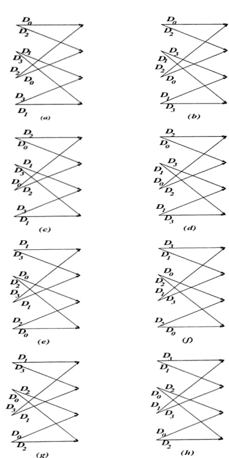
of rate R-\-l Lloyd-Max quantizer as tlie codewords, assigned to trellis branches according to Ungerboeck’s set ])a.rtitioning and branch labelling rules [52]. The system they introduced in [51] is given in Figure 2.'^1. The trellis can be any of Ungerboeck’s amplitude modulation trellises [52]. But the branches ])resented here no more represent single transitions but multiple ones quantity of whicli is determined by the rate of the .system. Consider an encoding rate of 2. Then the rate 3 Lloyd-Max output ])oints (for uniform i.i.d. .source), which will be employed as the codewords aie as shown on real line in Figure 2.4. These codewords are partitioned into four subsets by labeling consecutive points with Do·, Di, D2, Do, D i, D2, D:i,... starting with tlie leftmost (most negative)

point and proceeding to the right. Then tliese sub.sets are assigned to the trellis branches following branch labelling rules of Ungerl)oeck [52]:

1. Parallel transitions are associated with codewords with maximum dis­ tance between them.

2. The branches originating from the same node should be labeled with subsets with maximum distance between them.

3. The branches terminating at the same branch should be labeled with subsets with maximum distance between them.

4. All codewords should be used with equal frequency in the trellis diagram.

The first rule is satisfied with the above .set partitioning. To satisfy second and third rules the subsets are grou])ed as Do with D2 and D\ with Do and these

groups are assigned to leaving and entering branches as shown in the figure. Fourth rule is already satisfied with this labeling.

This system is later modified l>y Marcellin and Fischer to incorjiorate ])re- diction and they introduced PTCQ in [51]. The trellis search algorithm they use in their predictive .system is the same as the search algorithm of Ayanoglu and Gray [19] for /? = 1 and an extension of it for higher rates, but in the design stage they do not train the codel)ooks and they do not u])date the predictor coefficients.

OID,.

Dj

, 1 ^ 2 ^3

■7 A -5 À -3 A - A A 3 A 5 A 7 A

8 8 8 8 8 8 8 8