A continuous speech recognition system for Turkish language based on triphone model

(1)

A CONTINUOUS SPEECH RECOGNITION SYSTEM FOR

TURKISH LANGUAGE

BASED ON TRIPHONE MODEL

by Fatma PATLAR

Istanbul Kultur University, 2009

THESIS

FOR THE DEGREE OF MASTER OF SCIENCE IN

COMPUTER ENGINEERING PROGRAMME

SUPERVISOR

(2)

ii

ABSTRACT

A CONTINUOUS SPEECH RECOGNITION SYSTEM FOR TURKISH LANGUAGE BASED ON TRIPHONE MODEL

PATLAR, Fatma

M.S. in Computer Engineering

Supervisor: Assist.Prof. Dr. Ertuğrul SAATÇİ August 2009, 73 pages

The field of speech recognition has been growing in popularity for various applications. Such recognition embedded applications include automated dictation systems and command interfaces. Embedding recognition to a product allows a unique level of hands-free usage and user interaction. Our main goal was to develop a system that can perform a relatively accurate transcription of speech and in particular, a Continuous Speech Recognition based on Triphone model for Turkish Language. Turkish is generally different from Indo-European languages (English, Spanish, French, German etc.) by its agglutinative and suffixing morphology. Therefore vocabulary growth rate is very high and as a consequence, constructing a continuous speech recognition system for Turkish based on whole words is not feasible. By considering this fact in this thesis, acoustic models which are based on triphones, are modelled as five state Hidden Markov Models. Mel-Frequency Cepstral Coefficients (MFCC) approach was preferred as the feature vector extraction method and training is done using embedding training that uses Baum-Welch re-estimation. Recognition is implemented on a search network which can be ultimately seen as HMM states connected by transitions and Viterbi Token Passing algorithm runs on this network to find the mostly likely state sequence according to the utterance. Also to make a more accurate recognition bigram language model is constructed. MATLAB is used in processing speech and The Hidden Markov Model Tool Kit (HTK) is used to train models and perform recognition.

(3)

iii The performance of this thesis has been evaluated using two different databases, one of them is more commonly formed TURTEL speech database that is used for speaker independent system tests and the other one is particularly formed weather forecast reports database that is used for speaker dependent system tests.

In recognition experiments, word accuracy of speaker independent system has been measured as 59-63 percent. After finding optimum value for decision tree pruning factor by try outs, system tests have been repeated again by using the language model and the optimum pruning factor. These adjustments improved the performance by 30-33 percent and word accuracy has reached to 92-93 percent for all tests.

While the word accuracy of the speaker dependent system tests on the single person database is between 89-93 percent, usage of the language model and the optimum decision tree pruning factor has resulted with an increase in the performance and the word accuracy has reached to 95-97 percent.

Keywords: Continuous Speech Recognition, Triphone, Hidden Markov Model, Language Modelling, Bigram language model

(4)

iv

ÖZET

ÜÇLÜ SES MODELLİ TÜRKÇE SÜREKLİ KONUŞMA TANIMA SİSTEMİ

PATLAR, Fatma

Yüksek Lisans, Bilgisayar Mühendisliği Bölümü Tez Yöneticisi: Yrd.Doç.Dr. Ertuğrul SAATÇİ

Ağustos 2009, 73 sayfa

Konuşma tanıma tabanlı uygulamaların popülaritesi her geçen gün daha da artmaktadır. Bu uygulamalara dikte sistemlerini ve komut arayüzlü sistemleri örnek olarak verebiliriz. Bir ürüne konuşma tanımayı entegre etmek kullanıcıya benzersiz bir kullanım kolaylığı ve etkileşim imkanı sunar. Bizimde buradaki asıl amacımız Türkçe için nispeten hassas çeviri imkanı sunacak geniş kelime dağarcıklı bir sistem tasarlamaktı. Türkçe, sondan eklemeli morfolojisiyle genel olarak Hint-Avrupa dillerinden (İngilizce, İspanyolca, Fransızca, Almanca vs.) farklıdır. Bu yapısı sözcük dağarcığında büyük bir artışa neden olmakta ve sonuç olarak Türkçe için kelime tabanlı sürekli konuşma tanıma sistemlerinin yapılabilirliği pek mümkün olmamaktadır. Bu gerçeğide göz önüne alarak, bu tezde, akustik modeller, beş durumlu Saklı Markov Modelleri olarak modellenmiş üçlü-sesler temel alınarak oluşturulmuşlardır. Özellik vektörü çıkarımı için Mel Kepstral Katsayılar yaklaşımı tercih edilmiş, eğitim ise Baum-Welch yeniden tahmin algoritmasını kullanan "gömülü eğitim" yöntemi kullanılarak yapılmıştır. Tanıma işlemi bir arama ağı üzerinde işleyen Viterbi Token Passing algoritması kullanılarak gerçeklenmiştir. Bu arama ağı aslında model durumlarının geçişlerler birbirine bağlanmış hali olarak görülebilir. Aynı zamanda daha doğru bir tanıma yapabilmek için ikili dil modellemesi de uygulanmıştır. SMM‟i, “gömülü eğitim” kullanılarak eğitilmiş; tanıma kısmında ise “Andaç geçirmeli Viterbi algoritması” kullanılmıştır.

(5)

v Konuşmanın analizi ve işlenmesinde MATLAB; modellerin eğitimde ve tanımanın gerçekleştirilmesinde ise Hidden Markov Toolkit (HTK)‟den faydalanılmıştır.

Eğitim ve testlerde iki ayrı ses veritabanı kullanılmıştır. Genel amaçlı hazırlanmış olan TURTEL veritabanı kullanıcı bağımsız testlerde, daha özel amaçlı oluşturulan hava durumu tahmin raporları veritabanı ise kullanıcı bağımlı sistem testlerinde kullanılmıştır.

Konuşmacı bagımsız sistem tanıma testlerinde kelime doğruluk yüzdesi 59-63 olarak hesaplandı. Sistem performansını arttırmak için en uygun karar ağacı budama eşiği seçildi ve bunun sisteme dil modeli ile uygulanmasının ardından yüzde 30-33 arası artış sağlanarak doğruluk yüzdesinde 92-93 arasi değerler elde edildi. Kullanıcı bağımlı olan tek kişilik veritabanında yapılan testlerde doğruluk oranı yüzde 89-93 civarında iken, en uygun karar ağacının ve dil modelinin kullanılmasının doğruluk oranını yüzde 95-97'lere yükselttiği gözlemlendi.

Anahtar Kelimeler : Sürekli Konuşma Tanıma, Dil Modeli, Üçlü Ses, Saklı Markov Modeli, İkili Dil Modeli

(6)

vi To My Family

(7)

vii

ACKNOWLEDGEMENTS

I would like to express my appreciation, for their valuable supervision and his strong encouragement throughout the development of this thesis my advisor, Assist. Prof. Dr. Ertuğrul SAATÇİ.

I am most grateful to my family for everything and all my friends in the office and others for their patience, help and being very supporting and kind to me.

Finally, I would like to thank The Scientific and Technical Research Council of Turkey (TÜBİTAK, UEKAE) for support for my thesis.

(8)

viii

ASR

Automatic Speech Recognition

CSR

Continuous Speech Recognition

DFT

Discrete Fourier Transform

FFT

Fast Fourier Transform

MFCC

Mel Frequency Cepstral Coefficient

HMM

Hidden Markov Model

HTK

Hidden Markov Model Toolkit

The state transition probability

The observation symbol probability

The initial state

HMM Model

HMM States

Observation symbols Observation sequence Backward variable

Forward andBackward variables This partial probability

(13)

xiii

EQUATIONS

(2.1) Preemphasis Filter (2.2) Square Energy Algorithm (2.3) Rectangular Window (2.4) Hamming Window

(2.5) Fourier series and Coefficients (2.6) Discrete Fourier Transform (2.7) Mel Frequency

(2.8) Discrete Cosine Transformation

(2.9) HMM state transition probability distribution for each state (2.10) HMM observation symbol probability distribution

(2.11) HMM initial state distribution

(2.12) Forward Algorithm partial probability (2.13) Backward Algorithm partial probability (3.1) Observed speech waveform

(4.1) Percentage of correctly recognized words (4.2) Accuracy of recognition

(14)

1

INTRODUCTION

Speech Recognition is an active area of research for over sixty years and its popularity grows increasingly over the past years. Speech communication within human beings has played an important role because of its inherent superiority over other modes of human communication. As time passed, the need for better control of complex machines appeared and speech response systems have begun to play a major role in human-machine communication.

As technology created so many other ways of communication to human, nothing can replace or equal speech. In the past, human has been required to interact with machines in the language of those machines as they were not able to train them in the way of understanding human speech. With speech recognition and speech response system, human can communicate with machines using natural language human terminology.

The use of voice processing systems for voices input and output provides a degree of freedom for mobility, alternative modalities for command and data communication and the possibility of substantial reduction in training time to learn to interface with complex system. All those characteristics of speech yield lots of positive advantages over other methods of human-machine interaction, when incorporated into an effective voice control or voice data entry system [1].

In early 1970s commercial application of speech recognition started. Up to that time, as lots of advances have been made in the development of more powerful algorithms for speech analysis and classification. The extraction of word features to permit improved performance in isolated and connected word recognition and in the reduction of the cost of the related hardware has been the major goals of this field. Most successful speech recognition systems today use the statistical approach. The Hidden Markov Models are used to model speech variations in a statistical and stochastic manner [2]. The idea is collecting statistics about the variations in the signal over a database of samples, and uses these to make a representation of the stochastic process. The speech signal carries acoustic information about the symbolic translation of its meaning. The acoustic information is embodied in HMMs and sound events are modelled by them. Besides the acoustic information, the

(15)

2 sequence of the symbols also constitutes a stochastic process, which can also be modelled. Such statistical approaches to model the symbolic events are called language models.

There are few studies in Turkish speech recognition with respect to the most of the other languages. Especially the large vocabulary recognition field for Turkish is quite empty. The main reason for this is the difficulties caused by the Turkish language. Turkish is an agglutinative language which makes it highly productive in terms of word generation. This is an important problem for traditional speech recognizer which has a fixed vocabulary.

In real life this speech recognition technology might be used to facilitate for people with functional disability or can also be applied to many other areas. This leads to the discussion about intelligent computers and homes where could operate the light switch turn off/on, using computer without any contact to keyboard or operate some domestic appliances.

(16)

3

CHAPTER 1: SPEECH PROCESSING

1 BACKGROUND INFORMATION

1.1 Historical Knowledge on Speech Processing

It has been over 60 years since first works on the speech recognition and so much has been accomplished not only in recognition accuracy but also in performance factor.

For example in isolated word recognition, vocabulary sizes have increased from ten to several hundred words. Highly confusable words have been distinguished, improved adaptation to the individual speaker dependent and speaker independent systems have been developed, the telephone and noisy, distorting channels have been effectively used and effect of other environmental conditions like vibration, g-forces, and emotional stress have also been explored [3].

Historically, start and development of speech recognition researches can be summarized as follows;

The first serious attempt at automatic speech recognition was described by Dreyfus-Graf (in France) in 1950. In the „stenosograph‟ different sequences of sounds gave different tracks around the screen [3].

In 1952, Davis, Biddulph, and Balashek of Bell Telephone Laboratories developed the first complete speech recognizer.

Several years later, Dudley and Balashek (1958) developed a recognizer called “Audrey” that used ten frequency bands and derived certain spectral features whose durations were compared with stored feature pattern for words in the vocabulary. A major events in the history of speech recognition occurred in 1972, when the first commercial products appeared that word recognizer (100 Words / Phonological constraints), from Scope Electronics Inc, and from Threshold Technology Inc.

Early history of speech recognition: 1947: Sound Spectrograph

1952: Digits, using word templates, 1 speaker 1958: Digits, using phonetics sequences

(17)

4 1960: Digits, digital computer time normalization

1962: IBM Shoebox Recognizer 1964: Word recognizers for Japanese

1965: Vowels and consonants detected in continuous speech 1967: Voice actuated astronaut manoeuvring unit

1968: 54 Word recognizers, digit string recognizer 1969: Vicens reddy recognizer of continuous speech 1972: 1st Commercial word recognizer

100 Words / Phonological constraints 1974: Dynamic programming (200 Words) Telephone; Oxygen Mask

1975: Alphabet and Digits, 91 Words Multiple talker, No training

1976: ARPA Systems; HARPY, HEARSAY, HWIM 182 Talkers, 97% Accuracy, Telephone 1977: CRT Compatible voice terminal

1978: IBM Continuous Speech Recognizer

Spoken language systems technology has made rapid advances in the past decade of eighties, support by progress in the underlying speech and language technologies as well as rapid advances in computing technology.

As a result, there are now several research prototype spoken language systems that support limited interactions in domains such as travel planning, urban exploration, and office management. These systems operate in near real life, accepting spontaneous, continuous speech from speakers with no prior enrolment; they have vocabularies of 1000- 2000 words, and an overall correct understanding rate of almost 90%.

If we look at the speech recognition from Turkish Language perspective, there are only a few studies on Turkish speech recognition. Most of the studies were being done on isolated word recognition, where only a word is recognized at each search step [4] [5] [6] [7] [8].

(18)

5 Recently, large vocabulary continuous speech recognition systems are started to be studied. However, the performance of these systems are poor and not in the level of systems in other languages like English.

Similar or same methods used in English speech recognition generally also can be used in Turkish recognition. The acoustic modelling is almost universal for all languages, since the methods that are used yield similar results [9] [10] [11]. However, the classical language modelling techniques cannot be applied successfully to Turkish.

Turkish is an agglutinative language. Thus, great number of different words can be built from a base by using derivations and inflections [12]. The productive derivational and inflectional structure brings the problem of high growth rate of vocabulary. Furthermore, Turkish is a free word order language. So the language models that are constructed using the co occurrences of words do not perform well.

1.2 Speech Production System

Human communication is to be seen as a comprehensive diagram of the process from speech production to speech perception between the talker and listener

Figure 1 : Schematic diagram of the speech production [13]

The first element Speech formulation (A) is associated with the formulation of the speech signal in the talker‟s mind. This formulation is used by the Human Vocal Mechanism (B) to produce the actual speech waveform. The waveform is transferred via the air (C) to the listener. During this transfer the acoustic wave can be affected by external sources, for example noise, resulting in a more complex waveform.

(19)

6 When the wave reaches the listener‟s hearing system the listener percept the waveform (D) and the listener‟s mind (E) starts processing this waveform to comprehend its content so the listener understands what the talker is trying to tell him or her [13].

One issue with speech recognition is to simulate how the listener process the speech produced by the talker. There are several actions taking place in the listeners hearing system during the process of speech signals. The perception process can be seen as the inverse of the speech production process. Worth mentioning is that the production and perception is highly a nonlinear process [13]. To be able to understand how the production of speech is performed one need to know how the human‟s vocal mechanism is constructed.

The most important parts of the human vocal mechanism are the vocal tract together with nasal cavity, which begins at the velum. The velum is a trapdoor-like mechanism that is used to formulate nasal sounds when needed. When the velum is lowered, the nasal cavity is coupled together with the vocal tract to formulate the desired speech signal. The cross-sectional area of the vocal tract is limited by the tongue, lips, jaw and velum and varies from 0-20 [14].

Figure 2 :Human Vocal Mechanism [13]

When human produce speech, air is expelled from the lungs through the trachea. The air flowing from the lungs causes the vocal cords to vibrate and by forming the vocal tract, lips, tongue, jaw and maybe using the nasal cavity, different sounds can be produced.

(20)

7

1.3 Language and Phonetic Features

The speech production begins in the human‟s mind, when we form a thought that is to be produced and transferred to the listener. After having formed the desired thought, we construct a phase/sentence by choosing a collection of finite mutually exclusive sounds. The basic theoretical unit for describing how to bring linguistic meaning to the formed speech, in the mind, is called phonemes.

Phonetics is the study of the sounds of human speech. It is concerned with the actual properties of speech sounds (phones), and their production, audition and perception, while phonology, which emerged from it, studies sound systems and abstract sound units (such as phonemes and distinctive features). Phonetics deals with the sounds themselves rather than the contexts in which they are used in languages.

Turkish has an agglutinative morphology with productive inflectional and derivational suffixations. Since it is possible to produce new words with suffixes, the number of words is very high. According to [15], the number of distinct words in a corpus of 10 million words is greater than 400 thousand. Such sparseness increases the number of parameters to be estimated for a word based language model.

Language modelling for agglutinative languages needs to be different from modelling language like English. Such languages also have inflections but not to the same degree as an agglutinative language [16].

The Turkish alphabet contains 29 letters (45 phonetic symbols) and is a phoneme based language which means phonemes are represented by letters in the written language. There are 8 vowels and 21 consonants;

Vowels: a e ı i o ö u ü

Consonants : b c ç d f g ğ h j k l m n o ö p r s ş t v y z

There is nearly one to one mapping between written text and its pronunciation but some vowels and consonants have variants depending on the place they are produced in the vocal tract.

1.4 Speech Representation

The speech signal and all its characteristics can be represented in two different domains, the time and the frequency domain.

(21)

8 A speech signal is a slowly time varying signal in the sense that, when examined over a short period of time (between 5 and 100 ms), its characteristics are short-time stationary. This is not the case if we look at a speech signal under a longer time perspective (approximately T>0.5 s). In this case the signals characteristics are non-stationary, meaning that it changes to reflect the different sounds spoken by the talker.

The speech representation can exist in either the time or frequency domain, and in three different ways [14]. These are three-state representation, spectral representation and parameterization of the spectral activity.

1.4.1 Three-State Representation

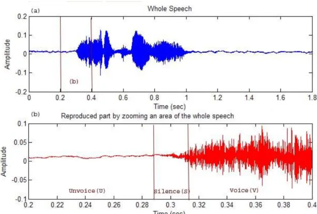
The three state representations is one way to classify events in speech. The events of interest for the three state representations are:

Silence (S) – No speech is produced

Unvoiced (U) – Vocal cords are not vibrating, resulting in a periodic or random speech waveform.

Voiced (V) – Vocal cords are tensed and vibrating periodically, resulting in a speech waveform that is quasi periodic.

Quasi periodic means that the speech waveform can be seen as periodic over short time period (5-100 ms) during which it is stationary. Stationary signals can be define constant in their statistical parameters over time.

(22)

9

Figure 3 : Three state representation

The upper plot (a) contains the whole speech sequence and in the plot (b) a part of the upper plot (a) is reproduced by zooming an area of the whole speech sequence. At figure the segmentation into a three state representation, in relation to the different parts of the plot(b), is given.

The segmentation of the speech waveform into well defined states is not straight forward. But this difficulty is not as a big problem as one can think. However, in speech recognition applications the boundaries between different state are not exactly defined and therefore non crucial.

As complementary information to this type of representation it might be relevant to mention that three states can be combined. These combinations result in three other types of excitation signals: mixed, plosive and whisper.

Mixed: Simultaneously voiced and unvoiced

Plosive: Start with a short region of silence then voiced or unvoiced speech, or both build up air pressure behind the closure, then suddenly release it.

(23)

10 1.4.2 Spectral Representation

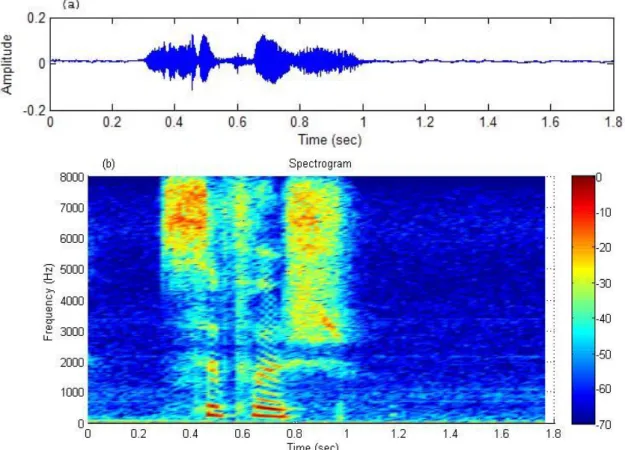
Spectral representation of the speech intensity over time is very popular and the most popular one is the sound spectrogram.

Figure 4 : Speech amplitude(a) and Spectrogram(b)

Here the darkest (dark blue) parts represents the parts of the speech waveform where no speech is produced and the lighter (red) parts represents intensity if speech is produced [17].

Figure (a) the speech waveform is given in the time domain and figure (b) shows a spectrogram in the time-frequency domain.

1.4.3 Parameterization of the Spectral Activity

When speech is produced in the sense of a time varying signal, its characteristics can be represented via a parameterization of the spectral activity. This representation is based on the model of speech production.

The human vocal tract can (roughly) be described as a tube excited by air either at the end or at a point along the tube. From acoustic theory it is known that the

(24)

11 transfer function of the energy from the excitation source to the output can be described in terms of natural frequencies or resonances of the tube, more known as formants. Formants represent the frequencies that pass the most acoustic energy from the source to the output. This representation is highly efficient, but is more of theoretical than practical interest. This because it is difficult to estimate the formant frequencies in low level speech reliably and defining the formants for unvoiced (U) and silent (S) regions.

1.5 Speech Recognition System

Recognition is the process of converting an acoustic signal, captured by a microphone or a telephone, to a set of words. The recognized words can be the final results, as for applications such as commands and control, data entry, and document preparation.

Speech recognition systems can be characterized by many parameters, some of the more important of which are speaking mode-style, vocabulary, enrolment etc. An isolated-word speech recognition system requires that the speaker pause briefly between words, connected word speech recognition similar to Isolated words, but with a minimal pause whereas a continuous speech recognition system does not. Spontaneous, or extemporaneously generated, speech contains disfluencies, and is much more difficult to recognize than speech read from script. Some systems require speaker enrolment a user must provide samples of his or her speech before using them, whereas other systems are said to be speaker-independent, in that no enrollment is necessary. Some of the other parameters depend on the specific task. Recognition is generally more difficult when vocabularies are large or have many similar-sounding words.

1.5.1 Categories of Speech Recognition 1.5.1.1 Recognition of Isolated Words

An isolated word recognition system operates on single words at a time, requiring a distinct pause between saying each word [18]. It requires about a half second (500ms) or greater pause be inserted between spoken words [19]. This is the simplest form of recognition to perform because the end points are easier to find and the pronunciation of a word tends not to affect others. Thus, because the occurrences of words are more consistent, they are easier to recognize. The technique of the system is to compare the incoming speech signal with an internal

(25)

12 representation of the acoustic pattern of each word in a relatively small vocabulary and to select the best match, using some distance metric [18]. Usually the recognition success is about 100% and it is adequate for many applications but is far from being a natural way of communicating [19].

1.5.1.2 Recognition of Connected Speech

Connected word recognition is one of the most interesting problems at the present stage of speech recognition research since isolated word recognition techniques have been improved up to a practically high level [20]. Connect word systems (or more correctly 'connected utterances') are similar to Isolated words, but allow separate utterances to be 'run-together' with a minimal pause between them [21]. 1.5.1.3 Recognition of Continuous Speech

A continuous speech system operates on speech in which words are connected together, i.e. not separated by pause. Continuous speech is more difficult to handle because of variety of effects [18]. First problem is to finding the utterance boundaries for allow users to speak almost naturally, while the computer determines the content. Another problem is co-articulation. The production of each phoneme is affected by production of surrounding phonemes, and similarly that the start and end of words are affected by preceding and following words. The recognition of continuous speech is also affected by the rate of speech [18]. Basically, these types of recognitions are named as a computer dictation.

(26)

13

CHAPTER 2: SPEECH TO TEXT SYSTEM

Speech recognition, also known as automated speech recognition (ASR) or speech-to-text (STT) is a process which converts the acoustic speech signal into written text. A typical example of speech to text application is in dictation systems. Speech to text systems may also be used as an intermediate step for making spoken language accessible to machine translation. Systems generally perform two different types of recognition: single-word and continuous speech recognition. Continuous speech is more difficult to handle because of a variety of effects such as speech rate, co-articulation, etc. Co-articulation express to changes in the articulation of a speech segment.

Speech to text systems can be separated into two categories which are speaker dependent and speaker independent. A speaker dependent system is developed to operate for a single speaker. These systems are usually easier to develop more accurate, but not as flexible as speaker independent systems. A speaker independent system is developed to recognize speech regardless of speakers, i.e. it does not need to be trained to recognize individual speakers. These systems are the most difficult to develop and their accuracy are lower than the speaker dependent systems. However, they are more flexible.

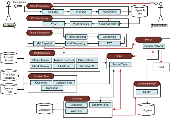
In this chapter we will explain general speech to text system frame and its modules. A general speech to text system involves several steps that can be categorized as follows: Data Preparation, Pre-Processing, Feature Extraction, Training and Recognition. Additional to this language model can be adapted to increase the performance of the system. Block Diagram of a speech to text system can be given as shown:

(27)

14 Speech file N-gram Dictionary Acoustic Model Transition Probability Decision Tree

AudioIO WaveIO WaveFileIO

State Element

Mel Cepstral Mel Frequency FFT Preemphasis Noise Cancelling

Frame Blocking Windowing

Search Network Questions Decision Tree Clustering HMM Set Mixture Element Transition P. HMM Element Observation P. Bigram Data Preperation Pre Processing Feature Extraction Model Creation VAD Language Model Dictionary Word List Decision Tree Search Dictionary Grammar File Microphone Model Train Train Training Recognition TEXT

Figure 5 : Speech Recognition Process

2.6 Preprocessing

Preprocessing is a process of preparing speech signal for further processing or in the other words to enhance the speech signal. The objective in the pre-processing is to modify the speech signal in such a way that will be more suitable for the feature extraction.

Preprocessing involves three steps: noise cancelling, preemphasis and voice activation detection.

Noise Cancelling Voice Activation

Detection Preemphesis Clean Speech Unvoiced-Voiced speech Preprocessing Speech Voiced speech

(28)

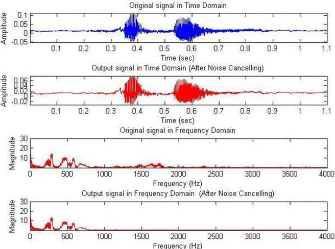
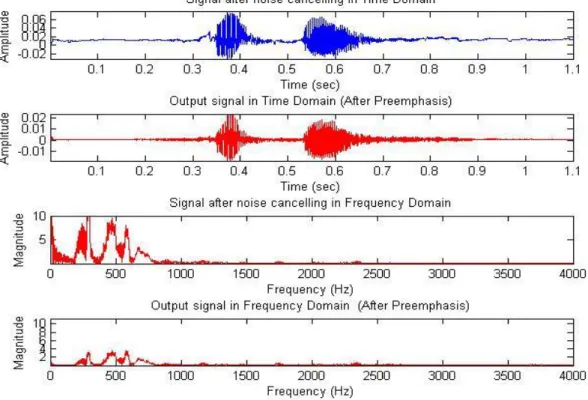
15 Noise Cancelling: Noise-cancelling reduces unwanted ambient sounds by a low pass filter which is a filter that passes low-frequency signals. Human can produce sounds between 100-4500Hz and for speech production the range is smaller. Thus, if telephone records (at 8000 Hz) are used, less than 120 Hz and above 3400 Hz can be a logical cut-off because over the 3400 Hz human speech has no information.

Figure 7 : Effect of the noise cancelling (word record is sIfIr (zero))

Preemphasis: The first stage in MFCC feature extraction is to boost the amount of energy in the high frequencies. It turn s out that if we look at the spectrum for voiced segment like vowels, there is more energy at the lower frequencies than at the higher frequencies. This drop in energy across frequencies (which is called spectral tilt) is caused by the nature of the glottal pulse. Boosting the high frequency energy makes information from these higher formants more available to the acoustic model and improves phone detection accuracy [22].

(29)

16 This is usually done by a highpass filter. The most commonly used filter type for this step is the FIR filter. The filter characteristic is given by the equation (2.1):

(2.1)

The value (a) is chosen to be approximately 0.95. There are two reasons behind this [23]. The first is that to introduce a zero near z=1, so that the spectral contributions of the larynx and the lips have been effectively eliminated.

Figure 8 : The effect of Preemphasis Filter in Time and Frequency Domain (word record is sIfIr)

By this way, the analysis can be asserted to be seeking parameters corresponding to the vocal tract only. The second reason, if the speech signal is dominated by low frequencies, preemphasis is used to prevent numerical instability [24].

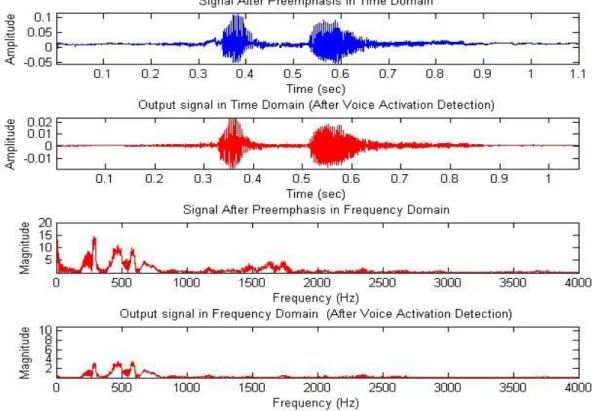
Voice Activation Detection: An important problem in speech processing is to detect the presence of speech in a background noise. This problem is often referred to as the end point location problem [25] [16].

(30)

17 The accurate detection of a word start and end points means that subsequent processing of the data can be kept to a minimum. In order to decide start and end points of a speech signal, the energies of each block is calculated first using sum of square energy algorithm.

(2.2)

Assuming that there is no speech in the first few frames, of recording, the average of the first few frames, give the maximum energy and the minimum energy which are used calculates for cutting down unvoiced parts of speech.

Figure 9 : The preemphasized signal cut down by the VAD.

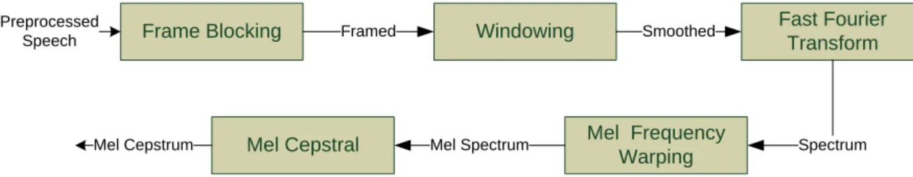
2.7 Feature Extraction

The purpose of feature extraction is to convert the speech waveform to some type of parametric representation (at a considerably lower information rate). The speech signal is a slowly time varying signal (it is called quasi-stationary) [26]. When examined over a sufficiently short period of time (typically between 20 and 100 ms), its characteristics are fairly stationary. However, over long periods of time (on the order of 0.2s or more) the signal characteristics change to reflect the different speech sounds being spoken.

(31)

18 Therefore, short-time spectral analysis is the most common way to characterize the speech signal. A wide range of possibilities exist for parametrically representing the speech signal for the recognition task, such as Linear Prediction Coding (LPC), Mel-Frequency Cepstrum Coefficients (MFCC), and others. MFCC is perhaps the best known and most popular, and this feature has been used in this work.

MFCC‟s are based on the known variation of the human ear‟s critical bandwidths with frequency. Linear prediction coefficients are mainly focused to model vocal tract while extracting feature coefficients from the speech, but MFCC‟s apply Mel scale to power spectrum of speech in order to imitate human hearing mechanism.

The MFCC technique makes use of two types of filter, namely, linearly spaced filters and logarithmically spaced filters. To capture the phonetically important characteristics of speech, signal is expressed in the Mel frequency scale. This scale has a linear frequency spacing below 1000 Hz and a logarithmic spacing above 1000 Hz. Normal speech waveform may vary from time to time depending on the physical condition of speakers‟ vocal cord. Rather than the speech waveforms themselves, MFFCs are less susceptible to the said variations [26] [34].

Frame Blocking

Mel Cepstral Mel Frequency

Warping

Fast Fourier Transform Windowing

Framed Smoothed

Mel Spectrum Spectrum

Preprocessed Speech

Mel Cepstrum

Figure 10 : Feature Extraction Steps

In a typical Feature Extraction process, the first step is windowing the speech to divide the speech into frames. Since high frequency formants have smaller amplitude than low frequency formants, high frequencies may be emphasized to obtain similar amplitude for all formants [4]. After windowing, magnitude squared FFT is used to find the power spectrum of each frame. Here we perform filter bank processing to the power spectrum, which uses mel scale. Discrete cosine transformation is applied after converting the power spectrum to log domain in order to compute MFCC.

(32)

19 2.7.1 Frame Blocking

Speech signals change in every few millisecond, because of this speech should be analyzed in small duration frames. Spectral evaluation of signals is reliable in case the signal is assumed to be stationary. Speech characteristics do not change much in a short time period because of this, speech signal is blocked into frames of N samples (generally between 20 and 100 millisecond), with adjacent frames being separated by M (M<N). The first frame consists of the first N samples. The second frame begins M samples after the first frame, and overlaps it by N-M samples. This process continues until all the speech is accounted for within one or more frames. Typical values for N and M are N=256 (which is equivalent to ~30 ms) and M=100.

2.7.2 Windowing

Choosing a window type is an important factor to process signal correctly. Two competing factors exist in this choice.

One of them is smoothing the discontinuity at the window boundaries and other factor is not to disturb the selected points of the waveform. Typical window types are Rectangular, Hamming and Hanning.

Indeed the simplest window is the rectangular window. The Rectangular window can cause problems, because it abruptly cuts of the signal at its boundaries. These discontinuities create problems when we do Fourier analysis. For this reason, a more common window used in MFCC extraction is the Hamming window, which shrinks the values of the signal toward zero at the window boundaries, avoiding discontinuities.

Windowing is also beneficial to eliminate possible gaps between frames. Without windowing, the spectral envelope has sharp peaks and the harmonic nature of a vowel is not apparent.

Definitions Rectangular Window (2.3) and the Hamming Window (2.4); are given as follows;

(2.3)

(33)

20 Where:

N is the number of samples in each frame (frame size) n is the index of the frames

The length of the window determines the frequency resolution of the signal. Increasing resolution is equal to using longer window, but in this case we may violate the assumption of stationarity for signals. Typically 10-25 ms windows are used in the processing.

2.7.3 Fast Fourier Transform

The next step is to extract spectral information for our windowed signal; we need to know how much energy the signal contains at different frequency bands.

In here Fast Fourier Transform(FFT) is used to convert speech frame to its frequency domain representation, the short term power spectrum is found. The FFT is a faster version of the Discrete Fourier Transform (DFT). The FFT utilizes some clever algorithms to do the same thing as the DFT, but in much less time. The Fourier series and DFT are defined by the formulas:

(2.5)

k=0,...,N-1 (2.6)

Evaluating this definition directly requires O( ) operations: there are N outputs , and each output requires a sum of N terms. An FFT is any method to compute the same results in O(N log N) operations. More precisely, all known FFT algorithms require Θ(N log N) operations.

2.7.4 Mel Frequency Cepstrum Coefficient

The most widely used feature vector in automatic recognition is so far known as mel frequency coefficients. These coefficients apply mel scale to power spectrum of speech in order to imitate human hearing mechanism.

Mel-Frequency Cepstral Coefficients (MFCC) are used in speech recognition because they provide a decorrelated, perceptually-oriented observation vector in the cepstral domain.

(34)

21 2.7.5 Mel Filter Bank

Magnitude squared FFT will be an information about the amount of energy at each frequency band. Human hearing however is not equally sensitive at all frequency bands. It is less sensitive at higher frequencies, roughly above 1000 Hertz.

In general the human response to signal level is logarithmic; humans are less sensitive to slight differences in amplitude at high amplitudes than at low amplitudes. (In other words logarithm compresses the dynamic range of values, which is a characteristic of human hearing system [27].)

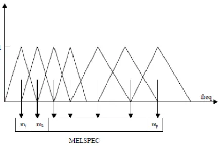
A mel is a unit of pitch defined so that pairs of sounds which are perceptually equidistant in pitch are separated by an equal number of mels. The mapping between frequency in Hertz and the mel scale is linear below 1000 Hz and logarithmic above 1000 Hz.

So a perceptual filter bank (a Mel-scale filter bank Eq.(2.7) and Figure below) is used to approximate the human ear‟s response to speech (in an attempt to receive only relevant information). Due to the overlapping filters, data in each band highly correlated. Filters are used to emphasize some of the frequency contents in power spectrum of the speech like ear does. More filter in the bank process the spectrum below 1 kHz since the speech signal contains most of its useful information such as first formant in lower frequencies.

Each filter output is the sum of its filtered spectral components [27].The central frequency of each Mel filter in the bank uniformly spaces below 1 kHz and it follows a logarithmic scale above 1 kHz. On the other hand these triangular filters are equally spaced along the Mel scale which is approximated by:

(2.7)

(35)

22

Figure 11 : Mel scale Filter Bank

The spacing between the filters in mel scale is computed using:

: The maximum frequency value in the filterbank in mels : The minimum frequency value in filterbank in mels : Number of desired filters

Center frequencies of the filters are found using:

After converting these center frequencies to Hertz, the filter are formed using the formulae below:

(36)

23 Then these filters applied to the magnitude spectrum and logarithm is taken:

2.7.6 Discrete Cosine Transformation

After filtering, discrete cosine transform (DCT) is applied to the resulting log filter-bank coefficients to compress the spectral information into lower order ones, and also to de-correlate them. DCT is formulates as:

(2.8)

Where N is the number of filter-bank channels, mj is the output of the j‟th filter and M is the number of DCT coefficients.

For speech recognition purposes, generally the first 12 coefficients are enough for getting information about the vocal tract filter which is cleanly separated from the information about the glottal source [22].

2.8 Training and Recognition

In Training and Recognition part, different methods have been tried by different researchers so far in order to find a better method to be used in speech processing applications [28] [23]. Some of these methods are seen to work better and are used frequently we can divide these methods into two classes:

First class, deterministic models that exploit some known specific properties of the signal, e.g., that the signal is a sine wave which has parameters like amplitude, frequency [28].

Second class of signal models is the set of statistical models in which one tries to characterize only statistical properties of the signal such as Gaussian processes, Poisson processes, Markov processes and Hidden Markov processes, among others.

For speech processing, both deterministic and stochastic signal models have had good success. There are advanced techniques in speech recognition such as Dynamic Time Warping (DTW), the Hidden Markov Modelling (HMM) and Artificial

(37)

24 Neural Network (ANN) techniques. The DTW is widely used in the small-scale embedded-speech recognition systems such as cell phones.

2.8.1 Dynamic Time Warping

Dynamic time warping is fundamentally a feature matching algorithm between a set of reference and test features [4]. The basic idea behind it is the time alignment of two sets. During DTW, it is tried to compress or expand the test feature set in a non-linear way to match it to a reference feature set. This is a critical task in template matching because the way of saying an utterance changes depending on the condition of speaker. The distance between the test and reference set is a measure of the goodness of the matching.

The disadvantage of this approach is the computational limitations. The DTW requires a template to be available for any utterance to be recognized and it is not used for complex task involving large vocabularies. The method can be effectively used in small scale applications.

2.8.2 Artificial Neural Networks

The application of artificial neural networks [23] to speech recognition is the newest and least well understood of the recognition technologies. The ANN approach is basically an alternative computing structure for carrying out the necessary mathematical operations. The ANN strategy can also enhance the distance or likelihood computing task by learning which features are most effective [23].

2.8.3 Hidden Markov Model

Nowadays a stochastic based method, Hidden Markov Modelling (HMM), is frequently used in large scale speech recognition systems. In this thesis one type of stochastic signal model, namely the Hidden Markov Model is concerned.

HMM is a finite-state machine with a given number of states; passing from one state to another is made instantaneously at equally spaced time moments. At every pass from one state to another the system generates observations. Two process taking place: the transparent one and the hidden one, which cannot be observed, first represented by the observations string and the second, represented by the states string [9]. Each state aims to characterise a distinct, stationary part of the acoustic signal. Phone or word models are then formed by concatenating the appropriate set of states. The hidden part of the HMM is the states process, which is governed by a Markov model.

(38)

25 We model such processes using a hidden Markov model where there is an underlying hidden Markov process changing over time, and a set of observable states which are related somehow to the hidden states [29].

An HMM is characterized by the following parameters and these are formally defined as follows:

N, the number of states in the model. For example, the HMM model for a phonetic recognition system will have at least three states which correspond to initial state, the steady state and the ending state [30]. The states will be denoted as

, and the state at time as .

M, the number of distinct observation symbols per state. In speech recognition systems, states are considered as the feature vector sequence of the model. The individual observation symbols will be denoted as

, the state transition probability distribution for each state.

(2.9)

,the observation symbol probability distribution in state .

(2.10)

,

the initial state distribution.

(2.11)

Having defined the necessary five parameters that are required for the HMM model ( ):

Speech is produced by the slow movements of the articulator organ that are the tongue, the upper lip, the lower lip, the upper teeth, the upper gum ridge, the hard palate, the velum, the uvula, the pharyngeal wall and the glottis. The speech articulators taking up a sequence of different positions and consequently producing the stream of sounds that form the speech signal. Each articulator position could be represented by a state of different and varying duration. Accordingly, the transition between different articulator positions (states) can be represented by .

(39)

26 The observations in this case are the sounds produced in each position and due to the variations in the evolution of each sound this can be also represented by

[31].

In the training mode, the task of the HMM based speech recognition system is to find a HMM model that can best describe an utterance (observation sequences) with parameters that are associated with the state model A and B matrix. A measure in the form of maximum likelihood is computed among the test utterance and the HMM, and the one with the highest probability value against the test utterance is considered as the candidate of the matched pattern [30].

Figure bellow a simple example of a five state left to right HMM. The HMM states and transitions are represented by node arrows, respectively.

S2 S3 S4 S1 S5 OT OT OT a12 Observation Sequence(OT) (Feature Vectors) b2 b3 b4 a22 a34 a23 a45 States (SN) :Hidden and

Transition probability A=(aij)

a33 a44

Observation Probability B=(bj)

Figure 12 : A five state left to right HMM

Basic Problems of HMM:

Once a system can be described as a HMM, three problems can be solved.

Problem 1 (Evaluation): Given the observation sequence and an HMM model, how do we compute the probability of given the model?

The probability of an observation sequence is the sum of the probabilities of all possible state sequences in the HMM. Native computation is very expensive. Given T observations and N states, there are NT possible state sequences. Even small HMMs, e.g. T=10 and N=10, contain 10 billion different paths. Solution to this and problem 2 is to use dynamic programming. Solution is Forward-Backward Algorithm. Problem 2 (Decoding): Given the observation sequence and an HMM model, how do we find the state sequence that best explains the observations?

(40)

27 The solution to Problem 1 (Evaluation) gives us the sum of all paths through an HMM efficiently. For Problem 2, we want to find the path with the highest probability. Solution is the Viterbi Algorithm.

Problem 3 (Learning): How do we adjust the model parameters , to maximize ?

Up to now we have assumed that we know the underlying model. Often these parameters are estimated on annotated training data, which has two drawbacks: 1. Annotation is difficult and/or expensive

2. Training data is different from the current data

We want to maximize the parameters with respect to the current data, i.e., we‟re looking for a model, such that the model best describes the observation sequence. Solution is Baum-Welch Algorithm.

Solutions to Basic Problems of HMM:

2.8.3.1 The Forward-Backward Algorithm

If we could solve the evaluation problem, we would have a way of evaluating how well a given HMM matches a given observation sequence. Therefore, we could use HMM to do pattern recognition, since the likelihood can be used to compute posterior probability , and the HMM with highest posterior probability can be determined as the desired pattern for the observation sequence [32].

The Problem 1 can be solved using the forward backward algorithm. The forward backward algorithm is an algorithm for computing the probability of a particular observation sequence [33].

Forward Algorithm:

The partial probability of state at time as - this partial probability calculates as;

(2.12)

We can solve the problem for inductively, using the following steps: Initialization;

(41)

28 Induction;

Termination;

Backward Algorithm:

The partial probability of state at time as - this partial probability calculates as;

(2.13)

i.e., the probability of the partial observation sequence from to the end, given state at time and model

.

Again we can solve for inductively, as follows: Initialization;

Induction;

The backward and the forward calculations can be used extensively to help solve fundamental problems 2 and 3 of HMMs.

2.8.3.2 Viterbi Algorithm

If we could solve the decoding problem, we could find the best matching state sequence given an observation sequence, or, in other words, we could uncover the hidden state sequence [32]. The viterbi algorithm is a dynamic programming algorithm for finding the most likely sequence of hidden states called the Viterbi path that results in a sequence of observed events [34].To find the single best state sequence, Q= { }, for the given observation sequence O= { }, we need to define the quantity [35]

(42)

29 i.e., is the best score (highest probability) along a single path, at time t, which accounts for the first t observations and ends in state . By induction [28]:

To actually retrieve the state sequence, we need to keep track of the argument which maximized (above equation), for each t and j. We do this via the array . The complete procedure for finding the best state sequence can now be stated as follows: 1) Initialization; 2) Recursion; 3) Termination:

4) Path (state sequence) backtracking:

2.8.3.3 Baum – Welch Algorithm

If we could solve the learning problem, we would have the means to automatically estimate the model parameters from an ensemble of training data [32].

The third, and by far the most difficult, problem of HMMs is to determine a method to adjust the model parameters ( ) to maximize the probability of the observation sequence given the model which maximizes the probability of the observation sequence. In fact, given any finite observation sequence as training data, there is no optimal way of estimating the model parameters. We can, however, choose

(43)

30 such that p(O| ) is locally maximized using an iterative procedure such as the Baum Welch method [28].

Firstly defined

,

the probability of being in state at time and state at time ,

(2.14)

The following figure illustrates the sequence of events leading to the conditions required by (2.14).

Figure 13 : Illustration of the sequence of operations required for the computation of the join

event that the system is in state at time t and state at time t +1 [28]

Definitions of the forward and backward variables, we can write in the form:

Where the numerator term is just and the division by gives the desired probability measure.

The probability of being in state at time , given the observation sequence and the model as:

Since accounts for the partial observations sequence and state at time , while accounts for the remainder of the observation sequence

, given state at , its relation with forward and backward variables can be given as [28]:

(44)

31 If we sum over , we get a quantity which can be interpreted as the expected number of times that state is visited and similarly the summation of over (from to ) can be interpreted as the expected number of transitions from state to state .

With the help of these, the formulas for re-estimating the parameters A, B and are given as [28];

So after re-estimation of the model parameters by using the current model , we will have a new model which is more likely to produce the observations sequence .

By using this procedure iteratively as in place of and repeat the re-estimation calculation, we then can improve the probability of being observed from the model until some limiting point is reached. In other words the iterative re-estimation procedure continues until no improvement in is achieved [28].

(45)

32

CHAPTER 3: EXPERIMENTAL WORK

In this chapter, the experimental work on continuous speech recognition system for Turkish Language based on Triphone Model will be presented.

The system uses MATLAB and Hidden Markov Model Toolkit (HTK) for data preparation, model training and recognition. The HTK is a free and portable toolkit for building and manipulating HMMs primarily for speech recognition research, although it has been widely used for other topics.

MATLAB is used for data preparation and preprocessing steps and HTK is used for implementing our system which has been used after completing the preprocessing step.

3.1 Data Preparation

Data Preparation is the first stage for building speech recognition system and includes the following steps:

3.1.1 Preparing Dictionary

Two different databases are used, one of them is more commonly formed TURTEL speech database which are collected at the acoustics laboratory of TÜBİTAK-UEKAE (National Research Institute of Electronics & Cryptology, The Scientific & Technical Research Council of Turkey), that is used for speaker independent system tests and the other one is weather forecast reports database that is used for speaker dependent system tests.

The goal of the system is to recognize weather forecast reports with a rate as high as possible. First of all, a word grammar about weather forecasting has to be formed to know which words will be recorded.

Then, every report passed through some preparation processes. First numbers changed to their text equivalents. Then all characters changed to their lower case versions, after that Turkish characters are changed with uppercase English ones like „ş‟ to „S‟, „ö‟ to „O‟ etc.

(46)

33

3.2 Recording the Data

Recording of training and test data are made using an ordinary desktop microphone and a laptop with a sampling rate of 8000 Hz, and with 8 bit quantization. Records have speech data consisting of words.

Since these records will be used in the other steps, contents of each file must be known. For this purpose a text file is created and associated with each record file. These files contain the text version of the recorded speech data: For example text file associated with a record of word “sIfIr” can be like this:

sIfIr

By using these files:

i. Dictionary file and word list file are formed.

ii. In offline and online recognition, results of the recognition are compared with the speech data in the records text file.

3.3 Preprocessing

Preprocessing is the process of preparing speech signal for further processing, in the other words to enhance the speech signal.

In preprocessing step, after enhancing speech signal (see Chapter 2 preprocessing) dictionary and word list files are formed. Word list file consists of the words in the record text files as one word per line:

Canakkale CankIrI Cevreleri Cevrelerinde. .

This file is used in forming dictionary file and the language model. Dictionary file consists of all the words in the word list. Format: all the file is an shown below: word [word representation] word pronunciation

For example a few lines from dictionary file can be like: CIG [CIG] C I G

(47)

34 OGle [OGle] O G l e

.

Dictionary file is used in training and recognition processes.

3.4 Feature Extraction

Feature extraction is performed after preprocessing steps. One important fact about the speech signal is that it is not constant from frame to frame. For this reason, speech must be converted into the parametric form. Block diagram all the feature extraction stages can be given as follows:

Preemphasis Window FFT Mel Filter

Bank Log Energy IFFT Deltas MFCC 12 Coefficient 1 Energy Feature 12 MFCC 12 Delta MFCC 12 Delta Delta MFCC 1 Energy 1 Delta Energy 1 Delta Delta Energy Speech

Signal

Figure 14: MFCC feature vector extraction process

Preemphasis:

This operation is used not to lose high frequency speech information of the incoming speech signal and also to make the signal spectrum flatter.

So, first, overall energy distribution of the signal is balanced in preemphasis stage by using a FIR filter ( ). The effect of this filter to the signal is:

By this way, it emphasized the high frequencies before processing. Also, the preemphasis filter is used to remove the spectral roll off which is caused by the radiation effects of the sound from the mouth.

The value for a usually ranges from 0.9 to 1.0. For our system, we choose a=0.95. We found an optimum value by trial and error.

(48)

35 Frame Blocking:

In this step the reemphasized speech signal is blocked into frames of N=200 samples (25ms) and each frame overlaps with the previous frame by a predefined size that in our case separated by M=80 samples ( 10 ms, typical to be stationary signal). The first frame consists of first 200 speech samples. The second frame begins 80 samples after the first frame, and overlaps it by 200-80 samples. Similarly, the third frame begins 2*80 samples after the first frame. Each signal is now converted into a set of fixed frames, with each frame is overlapping. The goal of the overlapping scheme is to smooth the transition from frame to frame.

Figure 15 : Frame blocking scheme

Windowing:

Each individual frame is windowed to minimize the signal discontinuities at the borders of each frame. We used the Hamming window which is far more successful than rectangular window in attenuating window edges. Hanning window can also be a choice. As can be seen from the figure that the difference is so small between Hamming and Hanning. For not violating the assumption of being stationary for signals a 25ms Hamming window is used. In our case every window has N=200 samples. (N is the number of samples per frame)

(49)

36

Figure 16 : Hamming Window

Figure 17 : Hanning Window

Fast Fourier Transform:

After the windowing step, we need to extract spectral information and know the energy amounts in each frequency band. FFT is used to convert each frame of N (200 samples) sample from the time domain to the frequency domain.

In order to lead FFT do it is job efficiently, N, point number, has to be a power of 2. Here N is selected as 256 points (200 samples ). Fast Fourier Transform is used with zero padding (256=200 samples+56 zero). Zero-padding append an array of zeros to the end of the input signal before FFT.

(50)

37 Zero-padding increases the number of data points to a power of 2 and provide better resolution in the frequency domain.

Mel Filter-Bank:

At this point, Speech signals have been transformed to the frequency domain and now frequency spectrum have to be converted to Mel spectrum. Because MFCC‟s apply Mel scale to the spectrum of speech in order to imitate human hearing mechanism.

It turns out that modelling this property of human hearing system during feature extraction improves speech recognition performance [22].

First the magnitude of the FFT components is computed, then this magnitude spectrum is multiplied with overlapping triangular filters in Mel scale.

In this work 26 triangular filters are formed to gather energies from frequenciy bands. They are all linearly spaced along Mel scale. According to the cut of 120hz-3400hz, 14 of these filter are below 1000hz and rest of them are above 1000hz.

Discrete Cosine Transform:

In the final step we use the DCT to convert the log mel-scale spectrum back to time domain.

When trying to recognizing phone identity the most useful information is the position and shape of the vocal tract. If we can know the shape of the vocal tract, we can determine which phone was produced. On the last step of the MFCC operation, by using DCT we separate the vocal tract information from the unnecessary (for phone detection) glottal source information. Generally the first 12 coefficients which we will get from DCT are enough for MFCC purposes. Higher cepstral coefficient can be used to determine pitch information.

Now we have Mel spectrum of the signal, next step is determining the Mel cepstral coefficients. To do this, logarithms of filterbank amplitudes are taken, and then using DCT, 12 DCT coefficients and 1 energy coefficient are calculated (39 size vector with 12 delta coefficients plus 1 energy and 13 double deltas).These coefficients are calculated in Mel scale and they are FFT based cepstral coefficients.

The main reason of preferring DCT rather than IFFT is IFFT requires complex arithmetic calculations compared to DCT.