Finding A Model Which Verifies The Appropriate Pattern For The Ovulation Data

Finding A Model Which Verifies The Appropriate Pattern For

The Ovulation Data

Suzan GAZIOGLU1

Abstract: The ovulation is the release of a mature egg from the female ovary. Normally,

in humans, only one egg releases at one time; occasionally, two or more erupt during the menstrual cycle. The egg erupts from the ovary on the 14th to 16th day of the approximately 28-day menstrual cycle. In about every four weeks of the active reproductive years, one follicle from only one of the two ovaries, left or right ovary, matures [1]. This study examines a dataset, which was obtained from 32 female human beings who were randomly selected from the population, and they had only one egg released at one time. The data is available from six cycles for each woman. The aim of this study is to find a model that verifies the appropriate pattern for the ovulation process of the females. Various models are suggested, and their pros and cons are discussed. The Markov chain model was found to be successful. The test results on this model has shown that the release of an egg from the female left or right ovary is dependent on just the previous cycle, and independent of the ones before the previous one.

Key words: Modeling; Markov chain; chi-square test; ovulation pattern.

Mevcut Veriler Kullanılarak Ovulasyon Paternini Tetkik Eden Bir Model

Elde Edilmesi

Özet: Ovulasyon (yumurtlama), dişi over folikülünden (dişi yumurtalığından) ovumun

(yumurtanın) atılmasına verilen addır. Normalde insanlarda bir seferde sadece bir yumurta atılır, nadiren bir menstrual siklusta iki veya daha fazla yumurta atılabilir. Ovum yaklaşık 28 gün süren menstrual siklusun yaklaşık 14. ile 16. günleri arasında atılır. Aktif üreme yılları boyunca her dört haftada bir sağ veya sol overlerden yanlızca birinde tek bir folikül gelişir [1]. Bu çalışma popülasyondan rastgele seçilen ve ayda yanlızca tek yumurta salınması ile karakterize 32 kadından elde edilen verilerle yapılmıştır. Bulgular her kadının 6 menstrual siklusundan elde edilmiştir. Bu çalışmanın amacı kadınlardaki ovulasyon paternini tetkik eden bir model bulmaktır. Çeşitli modeller öne sürülmüştür ve bunların avantajları ve dezavantajları tartışılmıştır. Makov zincir yöntemi başarılı bulunmuştur. Bu modeldeki sonuçlar göstermiştir ki, ovumun sağ veya sol overden atılması yanlızca önceki siklusa bağlıdır ama ondan önceki sikluslara bağlı değildir.

Anahtar kelimeler: Modelleme; Markov zinciri; Ki-kare testi; ovulasyon paterni.

1_{Department of Mathematics, Faculty of Arts and Sciences, University of Gaziosmanpasa, Tasliciftlik Campus, 60100} Tokat

Introduction

The ovulation is the release of a mature egg from the female ovary. Normally, in humans, only one egg releases at one time; occasionally, two or more erupt during the menstrual cycle. The egg erupts from the ovary on the 14th to 16th day of the approximately 28-day menstrual cycle. In about every four weeks of the active reproductive years, one follicle from only one of the two ovaries, left or right ovary, matures [1].

In this study, the data given in Table 1 belongs to 32 female human beings who were randomly selected from the population, and they had only one egg released at one time. There are six cycles for each of women that the data was obtained from. In the dataset, each row corresponds to one person, and ‘1’ is used to represent the egg which were from the right ovary, and ‘0’ is used for the left one. The aim of this study is to find a model that verifies the appropriate pattern for the ovulation process of the females.

Table 1. Ovulation Data*

m1 m2 m3 m4 m5 m6 Number _{of rt. of Runs}Number

0 0 1 1 1 0 0 1 1 0 0 1 1 1 0 0 1 0 1 1 1 1 0 1 0 1 0 0 1 1 0 0 0 0 1 0 0 1 0 1 1 0 1 1 0 1 0 0 1 1 0 1 0 1 0 0 0 0 0 1 1 1 0 0 0 0 0 0 1 1 0 1 0 0 1 0 0 1 1 1 1 1 0 1 0 1 0 0 0 0 0 1 1 1 0 1 0 0 0 0 1 0 1 1 0 0 1 0 0 1 1 1 1 1 1 1 1 1 0 0 1 0 0 1 0 1 1 0 0 0 0 0 1 1 1 0 0 0 0 0 1 0 0 1 0 1 0 1 1 1 0 1 1 0 0 1 0 1 1 0 0 0 0 1 0 1 1 0 1 0 0 0 1 0 1 1 0 0 1 1 1 0 0 0 1 1 0 1 0 1 1 0 0 0 2 2 4 4 3 4 3 0 3 2 3 4 3 4 4 4 3 6 4 5 0 2 3 2 0 5 3 6 3 1 1 1 2 3 4 4 2 2 3 1 3 2 3 2 4 2 2 3 5 1 3 2 1 4 2 3 1 2 2 1 2 3 17 14 15 17 14 15 92 76

Methods and Results

The following possible models comes to mind:

Model I. Alternating:

That is, getting the pattern ‘0 1 0 1 0 1’ or ‘1 0 1 0 1 0’ but that did not happen in the dataset in hand. Therefore, this type of model cannot be used here.

Model II. Alternating with the fixed number of months:

That is, varying between the subjects, but from the dataset it can be seen that that cannot be true for some of the females in the sample. Hence, we cannot use this model.

Model III.

X

_i is a sequence of independent Bernoulli trials with probability of

p

:

Here we have taken

p

as the probability of getting ‘1’ on a month, and it is denoted by

(

X

)

p

p

P

_ij

=

1

=

_ij

=

where

X

_ij is the result for person

i

(

1

≤

i

≤

32

)

,

month

j

For each person ~

iid

(

1

≤

j

≤

6

)

.

ij

X

Bin

( )

1 p

,

,

p

here can be estimated by

=

pˆ

(number of ‘1’s) (number of all ‘1’s and ‘0’s) = 0.479.

Hence, the confidence interval (0.408 , 0.549) is obtained. Because of the estimated

p

value, and the confidence interval above there is no reason to believe that the egg comes from the left or from the right ovary to be favored, and the data implies that the probability is the same for getting the egg from the left and from the right ovary. Therefore, it is reasonable to assume that the probability is 1/2 and try the following model, even though we could not rule this third model out completely.

Model IV.

X

_i is a sequence of independent Bernoulli trials with probability of 1/2:

If this model is true then the number of ‘1’s, (

1

), follows a binomial distribution with the parameters n = 6, and

i

X

≤

i

≤

32

p

= 0.5. But that does not mean that this model is the right one we are looking for. On the other hand, if we can conclude that does not have the binomial distribution, then that implies that model (IV) cannot be true.

i

X

Now we need to figure out if this model (IV) is the right one to go with. The following table has been produced by assuming that the model (IV) is true (see Table 2).

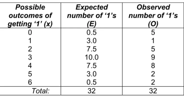
Table 2. Expected and observed numbers of ‘1’s Possible outcomes of getting ‘1’ (x) Expected number of ‘1’s (E) Observed number of ‘1’s (O) 0 1 2 3 4 5 6 0.5 3.0 7.5 10.0 7.5 3.0 0.5 5 1 5 9 8 2 2 Total: 32 32

The expected frequencies in Table 2 are computed according to the probability function of the Binomial distribution for all of the 32 females, i.e.,

( )

_p

x

(

_p

)

n x

x

n

x

p

E

_

⋅

⋅

−

−











⋅

=

⋅

=

32

32

1

where and

n

=

6

,

x

=

0

,

Κ

,

6

.

Table 3. Probability function

x P(x) with _{p = 0.5} Observed (O) P = O/n

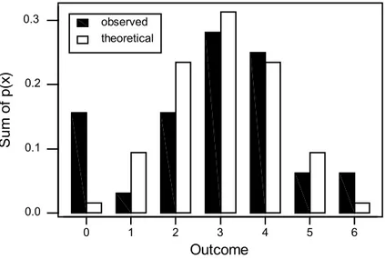
0 0.0156 5 0.1560 1 0.0940 1 0.0310 2 0.2344 5 0.1560 3 0.3125 9 0.2810 4 0.2344 8 0.2500 5 0.0940 2 0.0625 6 0.0156 2 0.0625

In Figure 1, the probability function in Table 3 is shown graphically.

observed theoretical 6 5 4 3 2 1 0 0.3 0.2 0.1 0.0 Outcome S um of p(x )

The bar chart in Figure 1, which displays both the probability distribution and the sample data frequency distribution, suggests the chi-square test.

Now we can perform chi-square test to test the null hypothesis of ~ for model (IV). We know that when we do the chi-square test the distribution of the test statistic

i

X

Bin

(

6

,

0

.

5

)

(

)

2 6 0 2

∑

=

−

=

i i i i

E

E

O

χ

can be approximated by a chi-square distribution with degrees of freedom

ν

= (number of cells free to vary) - (number of parameters estimated).

This approximation is considered acceptable, if all values are at least 5 [2]. As seen in Table 2, there are four expected values, which are less than 5. These cells can be combined so that all expected values are at least 5. Since it makes much more sense to combine the cells, which are right to each other, we combined 0 & 1

i

E

4

st _{and 5 & 6}th _{cells. Even we do that we get expected values}

of 3.5 for the both combinations, and it is still less than 5. We could combine 0 & 1 & 2 and 4 & 5 & 6 and collect each of them as one number, then we would have just 3 cells and due to that the degrees of freedom would be 2, hence the test would be less powerful. Since when we combine 0 & 1 and 5 & 6, we get 3.5 expected values, which is not very far below 5. Therefore, we will go with that combination. Then it is assumed that the test statistic can be approximated by a chi-square distribution with degrees of freedom of

2

χ

=

ν

. The test statistic is calculated to be 2.82. It is less than the mean of the distribution,

ν

=

4

, and then it has a big

p

value. Hence, we do not reject the null hypothesis of ~ but that does not mean that we accept , unless we do really believe in the binomial distribution here.

i

X

Bin

(

6

,

0

.

5

)

H

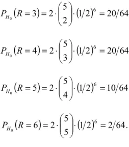
₀

The test we have done above focuses on the numbers of ‘0’s and ‘1’s. Our claim only indirectly addresses the relationship between one month and the next month. We know that the binomial distribution depends upon the independence but the test we have done does not directly address that. Now we want to know how we can be more directly advanced to gain the independence of one month to the next one. Since we believe that the runs directly address the independence we have decided to test the randomness of the runs. We assume that the events are independent. Here we have the null hypothesis of randomness. In order to derive a test for randomness based on the random variable R, the total number of runs, we need the probability distribution of R when the null hypothesis is true. The range of R is Range(R) =

{

. There are two ways to obtain a sequence. It can start with a ‘1’ or ‘0’, and we know that the number of different ways of distributing objects into

}

6

,

,

2

,

1

Κ

n

r

cells with no cell empty is and each of the

six months has the same probability of 1/2. Then the probability distribution of R when the null hypothesis is true can be derived as the following

,







1

1







−

−

r

n

(

)

( )

1

2

2

64

0

5

2

1

6 0



⋅

=











⋅

=

=

R

P

_H

(

)

( )

1

2

10

64

1

5

2

2

6 0



⋅

=











⋅

=

=

R

P

_H

(

)

( )

1

2

20

64

2

5

2

3

6 0



⋅

=











⋅

=

=

R

P

_H

(

)

( )

1

2

20

64

3

5

2

4

6 0



⋅

=











⋅

=

=

R

P

_H

(

)

( )

1

2

10

64

4

5

2

5

6 0



⋅

=











⋅

=

=

R

P

_H

(

)

( )

1

2

2

64

.

5

5

2

6

6 0



⋅

=











⋅

=

=

R

P

_H

As can be seen here, the probability distribution of R-1, which is the number of switches from ‘0’ to ‘1’ or from ‘1’ to ‘0’, is the binomial distribution, i.e., R-1 ~ when is true. Now, here a logical thing to do given that we have the 32 observations of the number of runs is to compare the sample distribution to the expected distribution. The values are given in Table 4. The expected values in the table are computed by multiplying the probability values given above by 32, the number of observations, and the counts, the observed values, are from the dataset.

(

5

,

1

/

2

Bin

)

H

₀

Table 4. The expected and the observed values. r Expected (E) Observed (O)

1 2 3 4 5 6 1 5 10 10 5 1 7 12 8 4 1 0

Since the first and the last expected values are less than 5, we combine 1 & 2 and 5 & 6 as we have done earlier. All the expected values are now greater than 5. Thus, the test statistic = 36.3 can be approximated by a chi-square distribution with the degrees of freedom

2

χ

ν

= 4–1=3 where 4 is the number of cells after we combined two pairs. The mean of the distribution is

µ

=

ν

= 3, and the standard deviation is

σ

=

2

ν

≅

2

.

4

. These results show that the test statistic is too way off scale. So the

p

value has to be near zero. Therefore, we reject the null hypothesis of randomness. The number of runs is too small, and they tend to be clustered. Then it is obvious that we did the right thing with not believing in model (IV) and doing another test when we did the first test for this model. Hence, we need a new model.

Model V. Markov chain, a sequence of events:

We know that a Markov chain is the probability of each of which is dependent on the event immediately preceding it, but independent of earlier events [3]. We suppose that whenever the

(

X

j

X

1

i

,

,

X

1

i

1

,

X

0

i

0

)

P

P

_ij

=

_n

=

_n−

=

Κ

=

=

where

i

= 0,1 ;

j

= 0,1 ; and

n

=

1

,

Κ

,

6

.

Then, we can state the following probabilities

(

X

1

X

1

1

)

p

1,1

P

_n

=

_n−

=

=

(

X

1

X

1

0

)

p

0,1

1

p

0,0

P

_n

=

_n−

=

=

=

−

(

X

0

X

1

1

)

p

1,0

1

p

1,1

P

_n

=

_n−

=

=

=

−

(

X

0

X

1

0

)

p

0,0

1

p

0,1

P

_n

=

_n−

=

=

=

−

.

As a strong assumption we believe that the probability of staying the same is equal to each other for each position and the probability of changing one position to the other is equal to

each other as well, i.e., Then, Due to that assumption, we

consider the transition times. We have five transition times between the six cycles. Here, we use S to denote the “switches” and N to denote the “no-switches”. Therefore, we can show the transitions for each female's situation as follows

,

0 , 0 1 , 1

p

p

=

1 , 0

p

=

p

_1,0

.

p

_0,1

=

p

_1,0

=

1

−

p

_1,1

.

1. N N N N N 2. N N N N N 3. N S N N N 4. S N N N S

and so on. Since it would not make any difference to deal with the number of switches or no-switches, we used N, the number of no-no-switches, to do the test in this study. The range of the

number of N’s is

{

We have known that R-1 ~ under , and (the number of

N’s)+1 gives us R, the number of runs. If the method (IV) were true, then we would state that the

number of N’s, which is denoted by #N, follows a binomial distribution with

n

and

but since we have already rejected the null hypothesis of randomness, and found out that the number of runs is too small, and they tend to be cluster, we know that the

}

.

)

5

,

1

,

0

Κ

Bin

(

5

,

1

/

2

H

₀

5

=

p

=

1

/

2

,

p

value is not 1/2. So we need to estimate the

p

value which should be greater than 1/2.

(

)

[

]

₀

_.

₇₂₅

5

32

32

76

5

32

ˆ

ˆ

ˆ

=

p

_1,1

=

p

_0,0

=

X

n

=

×

−

−

=

p

.

Our objective here is we are assuming that and we want to know if the sequence of events is a Markov chain. Then our null hypothesis is

,

1 , 1 0 , 0

p

p

=

0

H

: we have a Markov chain with

p

ˆ

_0,0

=

p

ˆ

_1,1

=

0

.

725

,

and the test statistics is the number of no-switches, #N. Each consecutive pairs is an independent Bernoulli trial with the probability of 0.725 for no-switches (or 0.275 for switches but here our probability value is 0.725 because our test statistic is the number of no-switches). So we can

identify our null hypothesis in terms of the binomial distribution, i.e., now the null hypothesis is #N ~

:

0

H

Bin

(

5

,

p

_1,1

)

.

In other words,

#N =

5

−

#S

=

5

−

(

R

−

1

)

=

6

−

R

~

Bin

(

5

,

0

.

725

)

.

Now we want to test for independence, then we are going to use test. The expected and observed values in this case are given in Table 5.

2

χ

Table 5. The expected and the observed values. r Expected (E) Observed (O)

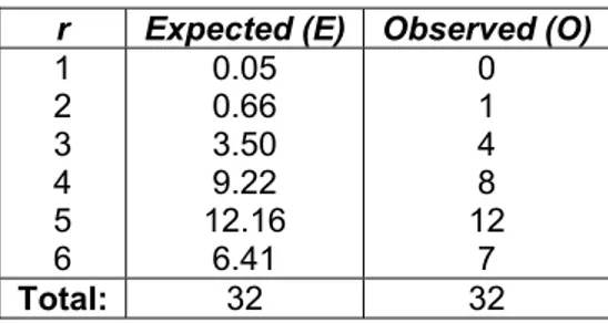
1 2 3 4 5 6 0.05 0.66 3.50 9.22 12.16 6.41 0 1 4 8 12 7 Total: 32 32

The expected values are computed according to the probability function of the binomial distribution for all of the 32 females as follows

(

)

r r

_p

p

r

E

_

⋅

⋅

−

−











⋅

=

5

1

5

32

where

r

=

0

,

Κ

,

5

, and

p

= 0.725. As we have mentioned above the distribution of the test statistic can be approximated by a chi-square distribution with the degrees of freedom

ν

=

4

if all

E values are at least 5, however here there are some E values less than 5. Having combined 0 & 1

& 2, the expected value is found to be 4.21. This value is still less than 5 but it is not very far below 5. Therefore, we can go with the combination of 0 & 1 & 2. The test statistics is found and the degrees of freedom after we combined the cells is

366

.

0

2

₌

χ

2

=

ν

. Since the test statistic value is less than the mean of the distribution, the

p

value has to be very big. Thus, we do not reject the null hypothesis of #N ~ Therefore, we can say that we have a Markov chain with the probability of 0.725.

(

5

,

0

.

725

)

.

Bin

Conclusion

As a result of all the models suggested and some tests were done about them in the previous part of this study, we have succeeded with the last model, the Markov chain model. As a result of this test we have found out that the release of an egg from the female left or right ovary is dependent on just the previous cycle, and independent of the ones before the previous one. As a conclusion, it is reasonable to say that if a female has a ‘0’ or ‘1’ on one month, she will get the same thing on the next month with a probability of 0.725.

[2] Mendenhall, W., Wackerly, D. D., Scheaffer, R. L. Mathematical statistics with applications. 4th Edition. Duxbury Press, California (1990).

[3] Ross, S. M. Introduction to probability models. 5th Edition. Academic Press Inc., Boston (1993).

Acknowledgement:

The dataset for this study has been provided by Donald White from Department of Mathematics of The University of Toledo.