A new solution algoritm for the transportation model

A NEW SOLUTION ALGORITM FOR THE

TRANSPORTATION MODEL

Sait PATIR*

Abstract

In this article, we have theoretically tried to solve the transportation model with a new algorithm and compare it with the existing solution methods. The solution aim of the trans-portation model is to meet the total demand and total supply in order to minimize the total cost. For this purpose, the problem can be solved by three methods. These methods are: North-West Diagonal method, Least Cost Method and Vogel’s method. The order of these methods in terms of giving the most optimal initial solutions is Vogel approach, Least Cost and North-West Diagonal. With this new algorithm and proposed two rules; the solution of the problem is much more optimal than the existing ones in case of the same values in the same column or rows and alternative ones. For this purpose, two model problems were first solved by the new method and then by Least Cost and Vogel method (without North-West Diagonal method); and then the results were compared. It was found out that the new algo-rithm gave the most optimal and the most suitable initial solutions. When we are applying Rule1 and Rule2 with Vogel method we get better result. It means that, we get nearer optimal solution than normal Vogel method. This method gives better result then other used methods. We can propose as an alternative.

Key Words: Transportation Model, New Algorithm, Optimal Value, Vogel’s App-roximate

1. INTRODUCTION

At the transportation model can define as m sources and n destinations. The amount of supply at source i is ai and the demand at destination j is bj.

The unit transportation cost between source i to destination j is cij.. Let xij

represent the amount transported from source i to destination j: then the LP model representing the transportation problem is given generally as (Hamdy,1987: 172-173).

Minimize z =

∑∑

∑

a

≤

∑

b

≥

In the 1939, the first paper is worked by the Russian Mathematic L.V.Kantrovich called “On the Translocation of Masses” about Transporta-tion Model (Kantrovich,1958; 1-4). Then, in the 1941, the second paper is worked by F.L. Hitchcock called “The Distribution of a Product From Seve-ral Sources to Numerous Localities” (Hitchcock,1941; 224-230). In the 1947, the four paper is worked by T.C. Koopmans called “ Optimum Utili-zation of the Transportation Systems” (Koopmans,1947; 24).

In the 1953, A. Charnes - W.W. Cooper (Cooper,1954; 49) and G.B. Dantzig (Dantzig; 1965; 13) are applied the first time “stepping-stone met-hod”. This method is developed by Churchman, Ackoff and Arnof (Church-man ve diğerleri,1966; 285).As different method is developed MODI (Modi-fied Distribution Method) by R.O.Ferguson (Ferguson,1955)t studying about this method have a let examples (Winston, 1994), (Wagner, 1969; 165-211), (Hillier and Lieberman,1986; 183-238).

Transportation Problems are two parts as balance and unbalances. Ba-lance problems are equality total demand with total supply. UnbaBa-lance prob-lems are not equality both total demand and total supply. So in a case dummy demand or dummy supply center is adding the problem. Dummy center transport cost is zero.

Transportation problems are solved three methods; the Northwest Cor-ner rule, Least cost and Vogel’s Approximation (Taha,age,182).

These problems have two optimality test; The Stepping Stone Method and MODI (Modified Distribution Method). We used to solve problems the MODI optimality test

Before, Example problems are solved with the new algorithm method and the MODI method is also doing the optimality test. Later, the same prob-lem is also solved with the least cost method and Vogel’s Approximate and optimality test is done with the Modified Distribution Method. That met-hod’s starting basic solutions and optimal stages were compared. Starting basic solution of the new algorithm is determined well than the other met-hods.

1.1 A NEW SOLUTION ALGORITM

The steps of the procedure are as follows and figure 1.;

Step 1. Find the cell containing the least cost in the first row. Search the column of this value, if there is a value less than this one in the column, take it. Then continue to row-column search and find the cell with the least cost.

Step 2. Meet the demand by taking into account the demand and supply to the last found value. If there are two equivalent values then apply the Rule 1.

Step 3. Apply the Step1 and Step 2 until meeting all the demands and supplies in the model.

Step 4. Stop the distribution in case of the equality.

Step 5. Pass on to optimality test. Apply the test until finding the best distribution.

Rule 1. If there are two equal values in the same row (column), elimina-te the risk by sending the goods with more cost (risk) and nearer to one of them.

— Is this column val-ue also the least cost its row?

— In the row the least value pole maximum goods

- Find the least cost at this row. - Is this value also

the least cost in the column

- At the column value is send to satisfied goods - Find the least cost in the first row.

- Is this value the least cost in the column?

No Yes

Return Yes

No

—At the row this element send to satisfied goods. Yes

- For this row find the least cost and send to be satisfied goods. - Return at par No Return Return Return

Until all demand with all supply is been satisfied, Repetition step1and step2.

Figure 1: New Solution Algorithm Procedure.

If all supply is all demand, stop the distribution.

Apply the Optimality Test

1.2. EXAMPLE ONE

It is solved blow a problem with the least cost method & Vogel’s App-roximate and back marking the new method. Table 1 is about in data prob-lem.

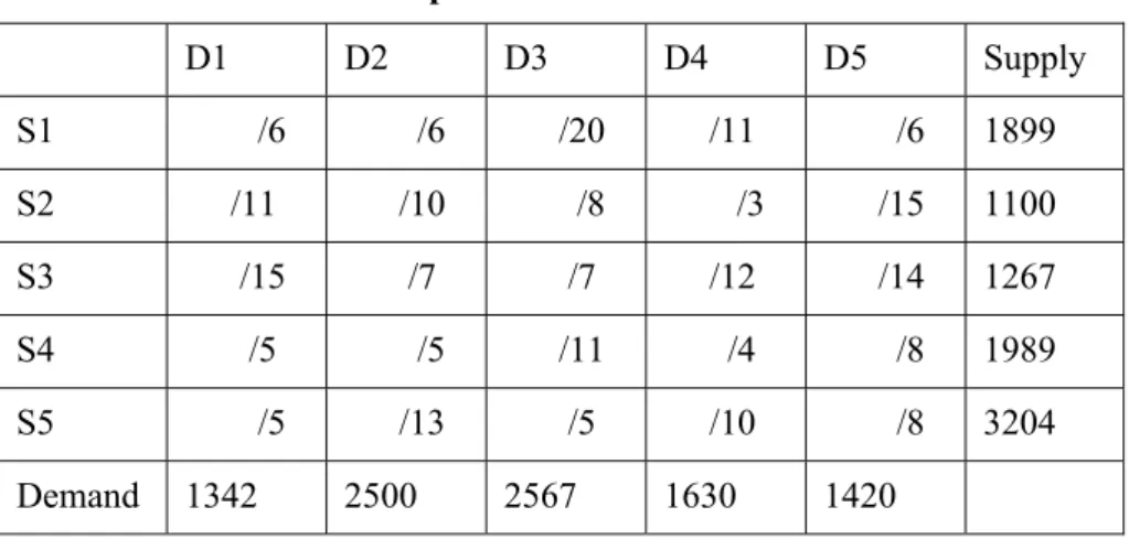
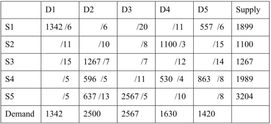
Table 1: Dates of example One

D1 D2 D3 D4 D5 Supply S1 /6 /6 /20 /11 /6 1899 S2 /11 /10 /8 /3 /15 1100 S3 /15 /7 /7 /12 /14 1267 S4 /5 /5 /11 /4 /8 1989 S5 /5 /13 /5 /10 /8 3204 Demand 1342 2500 2567 1630 1420

1.2.1. New Algoritm Solution

Example one solution procedure is below as;

Step 1; First row the least cost are three (X11, X12 and X15) the same

of six. Later, we’ll see those same numbers column. We come the five in the row. Here is the little four than five. We select column of four numbers. Here is the least number three. We select row of three numbers. Here is not the little than three. We send 1100 unite at X33 and this row not necessity, so it is eliminated. Again, we select four with vicious circle and send 530 units

Step2. Repetition, we go from six to five (X51 and X53). Here, we

se-lect the more cost column (X53). We send 2567 units (X53) and this column is eliminated. Again, we come (X41 and X51) the five. Here, we select the X51 and send 637 units, so this row is eliminate. Again, we go from first row to first column and X41 select the more cost than X42. Here is send 705 units and this column is eliminated. We select from two six to five column and send 1420 unit, so it is eliminated. Backward is second column. Here, we send (X12) 479 units and (X32) 1267 units. Now, Problem is equality total supply and total demand.

Step3. Because all supply and all demand are equalities, we stop to sol-ve the problem.

Step4. Stop the distribution.

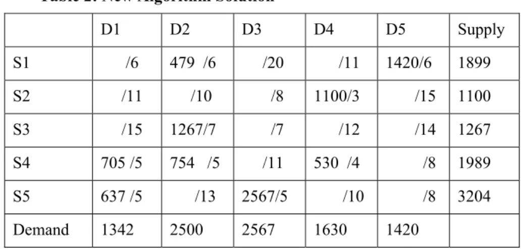
Solution of problem is Table2 below as.

Table 2: New Algorithm Solution

D1 D2 D3 D4 D5 Supply S1 /6 479 /6 /20 /11 1420/6 1899 S2 /11 /10 /8 1100/3 /15 1100 S3 /15 1267/7 /7 /12 /14 1267 S4 705 /5 754 /5 /11 530 /4 /8 1989 S5 637 /5 /13 2567/5 /10 /8 3204 Demand 1342 2500 2567 1630 1420 1.2.1.2. Optimality Test

- Modified Distribution Method (MODI)

Method tries to find for row and column index and present row index ui and column index vj. First row index is u1 equal to zero. ui + vj –cij = 0 ; Cij is

from i to j unit transport cost. From this equal is select maximum positive value. Its loop is done the first distance by plus (+) and second minus (-) sings. The leaving variable is then selected as the one having the smallest positive value. This value on the loop is from positive value (decrease) to negative value (increase) and the change will keep the supply and demand restrictions satisfied. Optimality test will repeat, until all different (. ui + vj – cij = 0 ) is been done to zero and negative

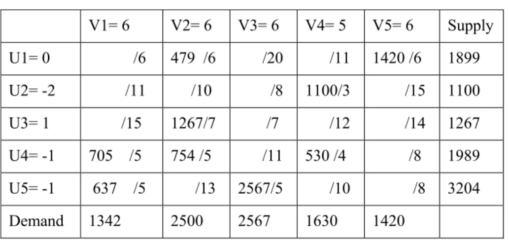
Optimality test at the MODI is follows as table 3.

Table 3: Index Values is Calculated

V1= 6 V2= 6 V3= 6 V4= 5 V5= 6 Supply U1= 0 /6 479 /6 /20 /11 1420 /6 1899 U2= -2 /11 /10 /8 1100/3 /15 1100 U3= 1 /15 1267/7 /7 /12 /14 1267 U4= -1 705 /5 754 /5 /11 530 /4 /8 1989 U5= -1 637 /5 /13 2567/5 /10 /8 3204 Demand 1342 2500 2567 1630 1420

U1+V1-C11=0; 0+6-6=0: U3+V1-C31=0; 1+6-15= -8: U5+V4-C54=0; -1+5-10=-11

U1+V3-C13=0; 0+6-20= -14: U3+V3-C33=0; 1+6-7=0: U5+V5-C55=-1+6-8=-1 U1+V4-C14= 0; 0+4-11= -7: U3+V4-C34=0; 1+5-12= -6: U2+V1-C21=0; -2+6-11=-7: U3 +V5-C35=0; 1+6-14= -7 : U2+V2-C22=0; -2+6-10= -6: U4+V3-C34=0; -1+6-11=-2: U2+V3-C23=0; -2+6-8= --4: U4+V5-C45=0; -1+6-8= -3 : U2+V5-C25=0, -2+6-15= -11: U5+V2-C52=0; -1+6-13= -8:

The problem is solved optimality test (MODI) and problem is optimal and total cost; 48998 YTL.

1.3. THE LEAST COST METHOD (LCM)

This method tries to select from the first row to end row the least cost at the cell and its send better goods. So it tries to equality with total supply and total demand.

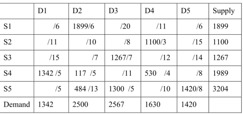
That problem one solves with the least cost method as, it is starting ba-sic solution table4.

Table 4: Starting Basic Solution With The Least Cost Method D1 D2 D3 D4 D5 Supply S1 /6 1899/6 /20 /11 /6 1899 S2 /11 /10 /8 1100/3 /15 1100 S3 /15 /7 1267/7 /12 /14 1267 S4 1342 /5 117 /5 /11 530 /4 /8 1989 S5 /5 484 /13 1300 /5 /10 1420/8 3204 Demand 1342 2500 2567 1630 1420 Optimality Test

Total cost is 57128 YTL. Problem one is done the optimality test (MODI), and after three stage problems is optimal total cost 48998. Distri-butor is follows as; X12= 479; X15=1420; X23= 1100; X32= 562; X33= 705; X42= 1459; X44= 530; X51= 1342, X53 1862.

1.4. VOGEL’S APPROXIMATE METHOD (VAM)

This method is a heuristic and the steps of the procedure are as follows (Taha, age,192-193).

Step 1.Evaluate a penalty for each row (column) by subtracting the

smallest cost element in the row (column)from the next smallest cost ele-ment in the same row (column).

Step 2.Identfy the row or column with the largest penalty, breaking ties

arbitrarily. Allocate as much as possible to the variable with the least cost in the selected row or column. Adjust the supply and demand and cross out the satisfied simultaneously, only one of them is crossed out and remaining row (column) is assigned a zero supply (demand). Any row or column with zero supply or demand should not be used in computing future penalties (in step 3).

Step3. a). If exactly one row or one column remains uncrossed out, stop.

b). If only one row (column)with positive supply (demand) remains uncrossed out, determine the basic variables in the row (column) by the least cost method.

c) If all uncrossed out rows and columns have (assigned)zero supply and demand, determine the zero basic by the least cost method. Stop.

d) Otherwise, recomputed the penalties for the uncrossed out rows and columns, then go to the step 2. ( Notice that the rows and columns with assigned zero supply and should not be used in computing these penalties.)

Rule 2: If a problem solving with the Vogel’s approximate selecting the same row& column have a lot of the same values, Rule 1 must use the solution

That problem of example two solves with the Vogel’s approximate is below as table 5; (not suggest two)

Table 5: With the Vogel’s Approximate Solve Starting of Problem

D1 D2 D3 D4 D5 Supply S1 1342 /6 /6 /20 /11 557 /6 1899 S2 /11 /10 /8 1100 /3 /15 1100 S3 /15 1267 /7 /7 /12 /14 1267 S4 /5 596 /5 /11 530 /4 863 /8 1989 S5 /5 637 /13 2567 /5 /10 /8 3204 Demand 1342 2500 2567 1630 1420

Beginning distributor cost is 57294. - Optimality Test

Beginning basic cost is 56713 YTL. Optimality test of problem is done with the MODI and after five stages; values are below as table 6.

Tablo 6: Optimality Test Result D1 D2 D3 D4 D5 Supply S1 479 /6 /6 /20 /11 1420/6 1899 S2 /11 /10 /8 1100/3 /15 1100 S3 /15 1041/7 /7 /12 /14 1267 S4 /5 1459 /5 /11 530 /4 /8 1989 S5 863 /5 /13 2567/5 /10 /8 3204 Demand 1342 2500 2567 1630 1420

This distribution total cost is 48998 YTL.

From here, if a problem has alternatives the same values, With New al-gorithm problem solving values will be better than the least cost method & Vogel’s approximate.

The same problem is solved with VAM adding Rule 1/2. The problem starting basic solution and optimality test is as follow table 7.

Table 7: Solutions with adding suggest one/two by the VAM

D1 D2 D3 D4 D5 S R/Penalty S1 1342/6 /6 /20 /11 557/6 1899 5/1414 _X S2 /11 /10 /8 1100/3 /15 1100 5/15 _X S3 /15 /7 1267/7 /12 /14 1267 5/5/716 _X S4 /5 1459/5 /11 530 /4 /8 1989 1/1/3 X S5 /5 1041/1 3 1300 /5 /10 863 /8 3204 3/3/3 Dem. 1342 2500 2567 1630 1420 C/Pen. 1/1 X 1/1/8 2/2 1/6 X 2/2/6

14 _{B. The same row have three same value (6) and selected to be the higher risk first column and}

eliminated. Later selected fifth column and this row is eliminated.

15 _{A. If penalties equality is select the least cost, this is two row and eliminated.}

Distribution cost is 59915 and after two stages the optimality test is 48998 as follow.X11=429; X15=1420; X34=1100; X32=1041; X33=226; X42=1459; X45=530; X51=863; X53=2341.

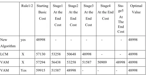
Solution to contribute to new algorithm & Rule1/2 compared the other methods below as Table 8.

Table 8: New Algorithm Solution Values Compare the Other Methods for Problem One

Rule1/2 Starting Basic Cost Stage1 At the End Cost Stage2 At the End Cost Stage3 At the End Cost Stage4 At the End Cost Sta-ge5 At The End Cost Optimal Value New Algorithm yes 48998 - - - - - 48998 LCM X 57130 53258 50648 48998 - - 48998 VAM X 57294 56438 53258 51587 50909 48998 48998 VAM Yes 59915 51587 48998 - - - 48998

We seem table 8, “new algorithm& Rule 1/2” solution to contribute di-rect. It seem “starting basic solution “of the new algorithm, optimal or the most near optimal. The other methods are further far than optimality. The least cost method need three stage for the optimal value and Vogel’s app-roximate need four stage for optimal value. But new algorithm is optimal the starting basic solution. In addition, when the same problem solving with the VAM is add to rule1-2, optimal procedures is seem to become shorter.

2. EXAMPLE TWO

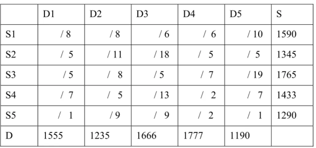
It is solved blow a problem with the least cost method and back mar-king the new method. Tablo9 is about in data problem.

Tablo 9: Example Problem Two Data D1 D2 D3 D4 D5 S S1 / 8 / 8 / 6 / 6 / 10 1590 S2 / 5 / 11 / 18 / 5 / 5 1345 S3 / 5 / 8 / 5 / 7 / 19 1765 S4 / 7 / 5 / 13 / 2 / 7 1433 S5 / 1 / 9 / 9 / 2 / 1 1290 D 1555 1235 1666 1777 1190

2.1. NEW SOLUTION ALGORITM

Step 1; First row the least cost are two (X13, X14) the same of six.

La-ter, we’ll see those same numbers column. These columns have two num-bers. From here, we come the one in the row. Here is the better risk X55 than X51. We select column of X55.We send at the X55; 1190 unite and later X51; 100 units, so X55 row is eliminated. Again, we select two with vicious circle and send 1433 units. This row is eliminated.

Step2. Repetition, we go from six to five (X33 and X31). Here, we

se-lect the more cost column (X33). We send 1666 units (X33) and X31 99 units. It is eliminated.. Again, we come (X21 and X24) the five. Here, we select the X21 and send 1345 units, so this row is eliminate. Again, we go from first row to first column and X14 select. Here is send X14; 344 units and X12; 1235this column is eliminated. We select from two six to five column and send 1420 unit, so it is eliminated. Now, Problem is equality total supply and total demand.

Step3. Because all supply and all demand are equalities, we stop to

sol-ve the problem.

Step4. Stop the distribution.

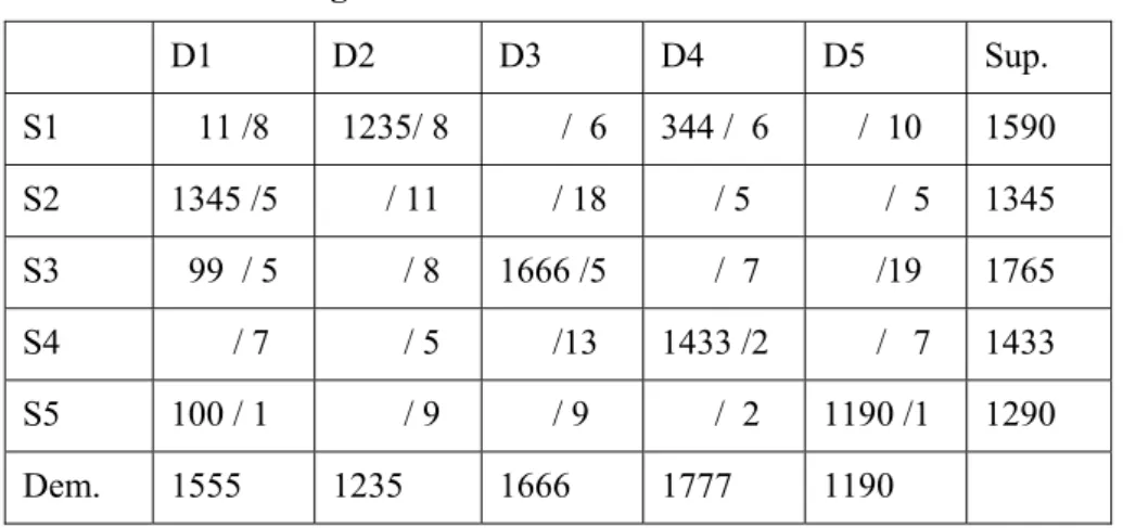
After here had new solution algorithm completed, Distribute was below as table 10.

Table10: Starting Solution With New Method D1 D2 D3 D4 D5 Sup. S1 11 /8 1235/ 8 / 6 344 / 6 / 10 1590 S2 1345 /5 / 11 / 18 / 5 / 5 1345 S3 99 / 5 / 8 1666 /5 / 7 /19 1765 S4 / 7 / 5 /13 1433 /2 / 7 1433 S5 100 / 1 / 9 / 9 / 2 1190 /1 1290 Dem. 1555 1235 1666 1777 1190

Total Distributing Cost= 37,738 YTL. -Optimality Test

After one stage was optimal with MODI and results as follows.

X12=1235; X13= 11; X14=344; X21=1345; X31= 110; X33= 1655; X44=1433; X51= 100; X55= 1190. Total Cost= 31,716 YTL.

2.2. THE LEAST COST METHOD

Example problem is solved with the least cost method in the table 11.

Table 11: Example problem is solved the least Cost method.

D1 D2 D3 D4 D5 S S1 111 /8 289 /8 /6 / 6 1190/10 1590 S2 45/ 5 /11 /18 / 5 / 5 1345 S3 99 / 5 / 8 1666 /5 / 7 / 19 1765 S4 / 7 946 / 5 /10 487 / 2 / 7 1433 S5 / 1 / 9 / 5 1290 /2 / 1 1290 D 1555 1235 1666 1777 1190

Total Cost= 38,934 YTL.

-Optimality Test

The problem was solved With MODI optimality test and after the four

stages, the problem had been optimality. Optimal results are below as;

X12=1235; X13= 11; X14=344; X21=1345; X31= 110; X33= 1655; X44=1433; X51= 100; X55= 1190.Total Cost= 31716 YTL.

2.3. VOGEL’S APPROXIMATION

The same problem is solved with Vogel’s approximate. Starting basic solution is below as table 12.

Table 12: Vogel’s Approximate Starting Basic Solution Values

D1 D2 D3 D4 D5 S S1 / 8 134 /8 1456 /6 / 6 / 10 1590 S2 / 5 /11 /18 155 / 5 1190 / 5 1345 S3 1555 /5 / 8 210 / 5 / 7 / 19 1765 S4 / 7 1101 / 5 /10 332 / 2 / 7 1433 S5 / 1 / 9 / 5 1290 / 2 / 1 1290 D 1555 1235 1666 1777 1190

Total Cost= 34,107 YTL. -Optimality Test

The Problem is done Optimality test and after three stages is optimal value below as;

X12=1235; X13= 355; X21=1001; X24= 344; X31=454; X33= 1311; X44=1433; X51=100; X55=1190, total cost= 31,716.

The same problem is solved with VAM adding comment1/2. The problem starting basic solution and optimality test is as follow table 13.

Table 13: The same problem is solved with VAM adding suggest one/two D1 D2 D3 D4 D5 S S1 / 8 234 /8 1356 /6 / 6 / 10 1590 S2 / 5 /11 /18 1345 / 5 / 5 1345 S3 1455/ 5 / 8 310 / 5 / 7 / 19 1765 S4 / 7 1001 / 5 /10 432 / 2 / 7 1433 S5 100 /1 / 9 / 5 / 2 1190/ 1 1290 D 1555 1235 1666 1777 1190

Starting basic solution total cost is 32,717 and after one stage is opti-mal value (31716).

Solution to contribute to new algorithm & Rule1/2 compared the other methods below as Table14.

Table 14: Solution of problems 2 is compared with new algorithm to other methods

Rule1/2 Starting Basic Cost Stage1 Cost Stage2 Cost Stage3 Cost Stage4 Cost Optimal Value New Algorithm yes 37738 31716 - - - 31716 LCM X 38934 33258 32038 31738 31716 31716 VAM X 34107 32917 32717 31716 - 31716 VAM Yes 32717 31716 - - - 31716

We seem table 14, “new algorithm& Rule1/2 ” solution to contribute direct. It seem “starting basic solution “of the new algorithm, optimal or the most near optimal. The other methods are further far than optimality.

CONCLUSION

New algorithm proved to solve the problems near the optimal. This method gives better results then other methods, so we can suggest new algo-rithm. If business transportation problems are not more dimension, we can suggest use new method. This new algorithm can be to economize the time and cost. Management makes to decision the short time the problems. It can help to solve the short time the translations problems for us. We can not suggest that if you use more dimensional problems, because we did not try how to get results.

REFERANSE

Hamdy, A.Taha., Operations Research An Introduction, Fourth Editions, Macmillan publishing Company, New York, 1987, p.172-173.

Kantrovıch, L.V., “On The Translocation of Masses”, Management Science, Vol.5, No.1, 1958, P.1-4.

Hıtchcock, F.L., “The Distribution of a Product from Several Sources to Numerous Localities”,

Journal of Mathematics and Physics, Vol.20, Part, 2.2.Aug.1941, p.224-230.

Koopmans, T.C., “Optimum Utilization of the Transportation Systems” Cowles Commission Paper, No: 24, (New Series), Proceedings of the International Statistical Conferens, Washington,1947.

Charnes, A. and W.W. Cooper “The Stepping Stone Method of Explaining Linear Program-ming Calculations in Transportation Problems” Management Science Vol.1. Oct. 1954-1955. p.49.

Dantzıg.G.B., “ Chaps,I-II-XX-XXI and XXIII” Activity Analysis of Production and Allocation In

the paper., T.C. Koopmans, Cowles Commission for Research in Economics Monograph

No: 13, New York, John Wiley and Sons Inc, 1965.

Churchman,C.W., R.I. Ackoff, E.I. Arnof., Introduction to Operations Research New York, John Wiley and Sons, Inc., 1966, p.285.

Fergison,R.O.., Linear Programming, New york, McGraw – Hill Book, Co., 1955.

Winston.W.L., Operations Research: Applications and Algorithms. 3.rd.Ed. PWS-KENT, Boston. Wagner. Harvey M. Principles of Operations Research with Applications to Management

Decisions, 1969, p.165-211.

Hillier. Frederic S., Lieberman Gerald J., Introduction to Operations Research, Fourth Edition, Holyday- Day,Inc. Oakland, Californıa, 1986, p.183-238.